Báo cáo hóa học: "Research Article Throughput versus Fairness: Channel-Aware Scheduling in Multiple Antenna Downlink" potx

Hindawi Publishing Corporation
EURASIP Journal on Wireless Communications and Networking
Volume 2009, Article ID 271540, 13 pages
doi:10.1155/2009/271540
Research Article
Throughput versus Fairness: Channel-Aware Scheduling in
Multiple Antenna Dow nlink
Eduard A. Jorswieck,
1
Aydin Sezgin,
2
and Xi Zhang
3
1
Communications Laboratory, Faculty of Electrical Engineering and Information Technology,
Dresden University of Technology, D-01062 Dresden, Germany
2
Department of Electrical Engineering & Computer Science, Henry Samueli School of Engineering,
University of California, Irvine, CA 92697, USA
3
ACCESS Linnaeus Center, Royal Institute of Technology, SE-100 44 Stockholm, Sweden
Correspondence should be addressed to Eduard A. Jorswieck,
Received 1 July 2008; Accepted 23 December 2008
Recommended by Alagan Anpalagan
Channel aware and opportunistic scheduling algorithms exploit the channel knowledge and fading to increase the average
throughput. Alternatively, each user could be served equally in order to maximize fairness. Obviously, there is a tradeoff between
average throughput and fairness in the system. In this paper, we study four representative schedulers, namely the maximum
throughput scheduler (MTS), the proportional fair scheduler (PFS), the (relative) opportunistic round robin scheduler (ORS),
and the round robin scheduler (RRS) for a space-time coded multiple antenna downlink system. The system applies TDMA based
scheduling and exploits the multiple antennas in terms of spatial diversity. We show that the average sum rate performance and the
average worst-case delay depend strongly on the user distribution within the cell. MTS gains from asymmetrical distributed users

whereas the other three schedulers suffer. On the other hand, the average fairness of MTS and PFS decreases with asymmetrical
user distribution. The key contribution of this paper is to put these tradeoffs and observations on a solid theoretical basis. Both
the PFS and the ORS provide a reasonable performance in terms of throughput and fairness. However, PFS outperforms ORS for
symmetrical user distributions, whereas ORS outperforms PFS for asymmetrical user distribution.
Copyright © 2009 Eduard A. Jorswieck et al. This is an open access article distributed under the Creative Commons Attribution
License, which permits unrestricted use, distribution, and reproduction in any medium, provided the original work is properly
cited.
1. Introduction
The optimal strategy for maximizing the sum capacity with
perfect channel state information (CSI) of a cellular single-
input single-output (SISO) multiuser channel is to allow
only the user having the best channel conditions in terms
ofSNRtotransmitateachtimeslot(TDMA).Thisresult
in [1] has induced the notion of multiuser diversity [2],
that is, the achievable capacity of the system increases with
the number of the users. The corresponding scheduling
policy is called maximum throughput scheduler (MTS). Sub-
sequently, TDMA-based channel-aware scheduling schemes
which consider temporal fairness [3] or stringent rate
constraints under energy efficiency [4]aredeveloped.
A major disadvantage of MTS is its unfairness toward
users at the cell edge. On the other hand, the most fair
but channel unaware scheduler is the round robin scheduler
(RRS) [5], that is, all transmissions take place in a strict
numerical order. The MTS and RRS leave room for various
channel aware schedulers that lie in between these two. In
order to increase the fairness for users at the cell edge, the so-
called proportional fair scheduler (PFS) can be applied. The
PFS weights the instantaneous transmission rates by their
averages to find the best user and achieves equal activity

probability for all users [6]. Yet another scheduler, which is
referred to as opportunistic round robin scheduling (ORS),
wasintroducedin[7]. It is a combination of the RRS and
MTS. The comparison of different schedulers with respect
to different performance criteria is a highly viable research
area. For instance, in [8], the throughput guarantee violation
probability is approximated and simulated for different
schedulers in different channel models. The asymptotic
throughput of channel-aware schedulers is analyzed in [9].
2 EURASIP Journal on Wireless Communications and Networking
In order to quantitatively measure the impact of the
scheduler on the fairness, different measures are proposed in
the literature [10–12]. The Jain fairness index (JFI) defined
in [10], also known as the global fairness index (GFI)
[13], provides a single number between zero and one that
measures the fairness even for resource scheduling in finite
windows. The average fairness defined in [11] is developed
from an information theoretic point of view. The worst-case
delay as it is used in, for example, [12] measures the average
number of transmissions needed until all users were active at
least m times.
Obviously, there exists a tradeoff between average
throughput and average fairness [14]. In this paper, we
study this tradeoff for the four scheduling algorithms MTS,
RRS, PFS, and ORS. The main novelty lies in the systematic
approach to this problem using majorization theory. This
tool helps understanding the impact of user distributions
within the cell on the system performance and on the average
worst-case delay. The application of majorization theory
allows to analytically and qualitatively assess the advantages

and disadvantages of the four channel-aware schedulers. The
contributions of the paper are as follows.
(1) In Section 2.5, closed form expressions for the four
scheduler for arbitrary nonsymmetrical user distri-
butions are derived.
(2) The impact of the user distribution on the average
sum rate is analyzed in Section 3, and it is shown that
the average sum rate is increased with asymmetrical
user distributions for MTS. For all other schedulers
(RRS, PFS, and ORS), it decreases.
(3) Different fairness measures and their properties are
discussed in Section 4. Furthermore, we study the
impact of the user distribution and its connection to
the service probabilities.
(4) The asymptotic performance for high SNR or large
number of users is analyzed in Section 5.
(5) In Section 6, the sum rate of MTS, RRS, and PFS
under a fixed rate constraint is derived, and the
impact of user distributionis characterized.
(6) In Section 7, we illustrate the theoretical results with
numerical single-cell multiuser simulations.
The paper is concluded in Section 7. Parts of the results for
single-antenna transmitter are presented without proofs in
[15]. The impact of interferer locations on the downlink
performance of the system is studied in [16].
2. System Model and Preliminaries
In this section, we present the system model, the channel
model, the measure of the user distribution based on
majorization, the high-SNR performance measures, and the
four scheduler. Our approach to the cross-layer analysis of

these scheduling algorithms is physical layer oriented.
2.1. System Model. In the signal model, there are K mobile
users which are served by a base station in downlink
transmission. The base station has multiple antennas (n
T
),
the mobiles have one antenna each. Denote the channels to
the users as h
1
, , h
K
. The base applies an OSTBC [17, 18]
in order to exploit spatial diversity without spatial feedback
overhead. Spatial feedback contains information about the
spatial signatures of the user channels, whereas channel
quality information contains scalar values . The data stream
vectors d
1
, , d
K
of dimension 1 × M of the K users are
weighted by a power allocation p
1
, , p
K
and added before
they come into the OSTBC as
x
1
, , x

M
. The output of the
OSTBC is a vector x
= [x
1
, , x
n
T
]ofdimension1× n
T
(compare to system model in [19]).Thecoderateisgivenby
r
c
= M/n
T
. Note that the framework can be extended also to
other code classes [20].
Each mobile first performs channel matched filtering
according to the effective OSTBC channel. Afterward, the
received signal at user k of stream n is given by
y
k,n
= a
k
K

l=1
x
l,n
+ n

k,n
,1≤ n ≤ M,(1)
with fading coefficients α
k
= a
2
k
=h
k

2
/n
T
,transmitstream
n intended for user l as
x
l,n
and noise for stream n as n
k,n
.
There are M parallel streams for each mobile. However, all
streams have the same properties in terms of a
k
and noise
statistics. Therefore, we restrict our attention without loss of
generality to the first stream n
= 1 and omit the index in the
following. Let p
k
be the power allocated to user k within one

block, that is, p
k
= E[|x
k
|
2
]. We assume a short-term power
constraint, that is,

K
k
=1
p
k
≤ P. The noise power at the
receivers is σ
2
. The transmit power is distributed uniformly
over the n
T
transmit antennas, and each data stream has an
effective power p
k
/n
T
. We incorporate this weighting into the
transmit SNR given by ρ
= P/n
T
σ

2
.
The mobiles feed back their scalar channel quality
indicators, that is, their fading coefficient a
1
, , a
K
to the
base and we assume these numbers are perfectly known at
the base station. As such, the base has perfect information
about the channel norm but not about the complete fading
vectors.
2.2. Channel Model. Thechannelvectorsh
1
, , h
K
are
modeled as independently zero-mean complex Gaussian
distributed vectors with covariance matrix c
k
I in rich
multipath environment. The variance c
k
depends mainly on
the distance of the user to the base, and it is called average
channel power. Therefore, the fading coefficients α
1
, , α
K
are independently χ

2
-distributed with n
T
complex degrees of
freedom weighted by the average channel power c
1
, , c
K
,
that is, using independent standard χ
2
n
T
-distributed random
variables w
1
, , w
K
, the fading coefficients are expressed as
α
k
= c
k
w
k
.
2.3. Measure of User Distr ibution. The distance of the mobile
k to the base station is determined by the average channel
power c
k

. In the following, we refer to the vector of average
EURASIP Journal on Wireless Communications and Networking 3
channel powers c
= [c
1
, , c
K
] as the user distribution. In
order to guarantee a fair comparison between different user
distributions, we constrain the sum variance to be equal to
the number of users, that is,

K
k
=1
c
k
= K. Without loss
of generality, we order the users in a nonincreasing way
according to their fading variances, that is, c
1
≥ c
2
≥···≥
c
K
. The constraint regarding the sum of the fading variances
verifies that we compare scenarios in which the channel
carries the same average sum power. We need the following
definitions [21].

Definition 1. For two vectors x, y
∈ R
n
, one says that the
vector x majorizes the vector y and writes x
 y if

m
k=1
x
k
≥

m
k=1
y
k
for m = 1, , n−1and

n
k=1
x
k
=

n
k=1
y
k
(note that

sometimes majorization is defined by the sum of the smallest
m components [22]).
The next definition describes a function Φ which is
applied to the vectors x and y with x
 y.
Definition 2. A real-valued function Φ defined on A
⊂ R
n
is said to be Schur convex on A if from x  y on A follows
Φ(x)
≥ Φ(y). Similarly, Φ is said to be Schur concave on A if
from x
 y on A follows Φ(x) ≤ Φ(y).
Majorization is a useful tool to study the impact
of vectors which can be partially ordered. The common
monotony properties of scalar functions correspond to the
Schur-convex property of vector functions. The reason for
the term “Schur-convex” instead of “Schur-monotone” is
that every symmetric and convex vector function is Schur-
convex. Majorization is a large and active area of research in
linear algebra, with entire books [21] devoted to its theory
and application.
It is worth mentioning that majorization induces only a
partial order on vectors with more than two components,
that is, not all possible vectors can be compared with each
other. This is due to the fact that vectors with more than two
components cannot be totally ordered. However, a sufficient
number of vectors can be compared. Also, the extreme cases
can be used for comparison with any other vector. For more
information about this measure of user distribution and its

application see [23, Section 4.2.1].
2.4. High-SNR Measures S
∞
and L
∞
. The quantitative
performance is analyzed using the high-SNR offset concept
from [24]. Denote by C(ρ) the average throughput as a
function of the SNR. The two high-SNR measures are
introduced as follows:
S
∞
= lim
ρ →∞
C(ρ)
log(ρ)
,
L
∞
= lim
ρ →∞

log(ρ) −
C(ρ)
S
∞

.
(2)
The measures S

∞
and L
∞
arereferredtoashigh-SNR
slope and the high-SNR power offset, respectively. At
high SNR, the average throughput behaves like C(ρ)
=
S
∞
((ρ[dB]/3dB) −L
∞
)+O(1). For convenience, these high-
SNR measures are defined in 3 dB units. For further discus-
sion, see [24, Section 2]. These two high-SNR measures are
useful if two systems are compared which differ either in their
multiplexing gain, that is, the slope of the average throughput
curve at high SNR, or which have equal S
∞
but are shifted at
high SNR.
2.5. Types of (Channel Aware) Scheduling. Since the base
station has only partial CSI in form of the channel norm, we
restrict all scheduling strategies to TDMA-based scheduling.
From the single-antenna downlink, it is well known that if
perfect CSI is available at the base station, the sum rate is
maximized by single-user transmission to the best user only
[1], that is, TDMA achieves the sum capacity. This result
leads to the notion of multiuser diversity and the concept
of opportunistic communication [2]. This scheduler is called
MTS, and the achievable average sum rate is given by

R
MT
sum
= E

log

1+ρ max
1≤k≤K


h
k


2

. (3)
Note that the average sum rate of the MTS can be written in
integral representation as
R
MT
sum
=

∞
0
ρ
1+ρt


1 −
K

k=1

1 −
Γ

n
T
,

t/c
k

Γ(n
T
)


dt,(4)
using the incomplete gamma function Γ(a, z)
=

∞
z
exp(−t)t
a−1
dt. The case with single-antenna base
and symmetrically distributed users (c

= 1) is studied in
[25]. The MTS is unfair from a user perspective because
mobiles at the cell edge have less probability to be served.
The opposite type of scheduler is the round robin
scheduler (RRS). It is not channel aware but it minimizes the
average worst-case delay, that is, the average time until every
user has been served at least once. The average sum rate is
given by
R
RR
sum
= E

1
K
K

k=1
log

1+ρh
k

2


= E

1
K

K

k=1
log

1+ρc
k
w
k


.
(5)
Note that (5)canberewrittenforn
T
= 1 in closed form as
R
RR
sum
=
1
K
K

k=1
Ei

1,
1
ρc

k

exp

1
ρc
k

,(6)
where the exponential integral is given by Ei(a, x)
=

∞
1
exp(−tx)t
−a
dt.
These two schedulers are the two most extreme cases.
The MTS maximizes the average sum rate, whereas the
RRS minimizes the average worst-case delay. A compromise
between the two is the proportional fair scheduler (PFS)
[2]. For the analysis, we use the so-called relative SNR
scheduler. The user is served which has the highest ratio of
4 EURASIP Journal on Wireless Communications and Networking
the instantaneous rate to average rate. Hence, the achievable
sum rate is given by
R
PF
sum
= E


log

1+ρ


h
k
∗


2

with k
∗
= arg max
1≤k≤K


h
k


2
c
k
.
(7)
In reality, the average transmission rate is updated from
transmission interval to transmission interval. Here, we use

the ergodic formulation of the scheduler (let the window
length t
c
→∞). Note that (7)canberewrittenas
R
PF
sum
=
1
K
K

k=1
E

log

1+ρc
k
max
1≤l≤K
w
l

,(8)
because the scheduling probability of all users is equal to 1/K.
For n
T
= 1, (8) can be rewritten in closed form as
1

K
K

k=1
K

l=1
(−1)
l−1
⎛
⎝
K
l
⎞
⎠
Ei

1,
l
ρc
k

e
(l/ρc
k
)
. (9)
Another interesting channel-aware scheduler is proposed
in [7]. The one-round version [26] of the relative oppor-
tunistic round robin scheduler (ORS) guarantees the same

average worst-case delay as the RRS but exploits a certain
amount of multiuser diversity. It consists of K rounds and
initializes the set of available users S with S
={1, , K}.
Within each step, the relative best user max
k∈S
(h
k

2
/c
k
)out
of the set of available users is picked and removed from the
set. After K steps, it is guaranteed that all users were active at
least once.
For our analysis, we need the representation in the
following lemma.
Lemma 1. The average sum rate of the ORS (13) can be
written as
R
OR
sum
=

∞
0

1 −
1

K
2
K

n=1
K

i=1

1 −
Γ

n
T
,

t/c
i

Γ(n
T
)

n

·
ρ
1+ρt
dt.
(10)

Proof. The CDF of the relative ORS is derived for n
T
= 1in
[27, Equation (6)] and is given by
P(t)
=
1
K
2
K

n=1
K

i=1

1 −e
−(t/c
i
)

n
. (11)
For general n
T
> 1, it reads
P(t)
=
1
K

2
K

n=1
K

i=1

1 −
Γ

n
T
,

t/c
i

Γ(n
T
)

n
. (12)
We use the integration by parts rule

b
a
f (x)g


(x)dx =
|
f (x)g(x)|
b
a
−

b
a
f

(x)g(x)dx. Now, identify f (x) = log(1 +
ρx)andg(x)

= p(x), respectively, with the pdf of the
relative ORS p(x). Choose carefully g(x)
= P(x) − 1to
assure existence of the first part. Then, we obtain finally the
representation in (10).
The sum rate performance for n
T
= 1 can be further
simplified as in [27, Equation (8)] to obtain the closed form
expression
R
OR
sum
=
1
K

2
K

n=1
n
K

i=1
n
−1

j=0
⎛
⎝
n −1
j
⎞
⎠
(−1)
j
·
e
((1+j)/c
i
)
1+j
Ei

1,
1+j

c
i

.
(13)
With the sum rate expressions in (4), (5), (8), and (10),
we are now ready for the analysis of the user distribution c in
the next section.
3. Analysis of Sum Rate Performance
In this section, we analyze the impact of the user distribution
on the sum rate performance of the four scheduler. One
main question is whether the standard assumption about
a symmetric user distribution, which is made often for
simplification, leads to an upper or lower bound on the real
system throughput. First, we present the theoretical results,
and then we discuss their meaning in the paper context.
3.1. Schur-Convexity and Schur-Concavity Properties. The
following result is provided in [28]forn
T
= 1and
restated and proved here for n
T
> 1. It states that a more
asymmetrical user distribution increases the average sum
rate with MTS.
Theorem 1. Let c and d be two different average user powers.
The average sum rate of the MTS is Schur-convex with respect
to user powers c and d,thatis,
c  d
=⇒ R

MT
sum
(c) ≥ R
MT
sum
(d). (14)
The proof can be found in [28, Theorem 1] for the single-
antenna n
T
= 1 case. We present in Appendix A the more
general proof for convenience.
The impact of the user distribution on the performance
of the RRS is analyzed in the next result.
Theorem 2. The average sum rate of the RRS is Schur-concave
with respect to the vector of average user powers c,thatis,
c  d
=⇒ R
RR
sum
(c) ≤ R
RR
sum
(d). (15)
Proof. Define the average sum rate as a function of c as
R
RR
sum
(c) =
1
K

K

k=1
E

log

1+ρc
k
w
k

, (16)
and check Schur’s condition [23] directly
∂R
RR
sum
(c)
∂c
1
−
∂R
RR
sum
(c)
∂c
2
= E

ρw

1
1+ρc
1
w
1

−E

ρw
2
1+ρc
2
w
2

≤
0.
(17)
EURASIP Journal on Wireless Communications and Networking 5
The impact of the user distribution on the performance
of PFS is derived analogously in Theorem 3.
Theorem 3. TheaveragesumrateofthePFSisSchur-concave
with respect to the vector of average user powers c,thatis,
c  d
=⇒ R
PF
sum
(c) ≤ R
PF
sum

(d). (18)
Proof. Start from the representation in (8) and check Schur’s
condition
∂R
PF
sum
(c)
∂c
1
−
∂R
PF
sum
(c)
∂c
2
=
1
K
E

ρc
1
max
1≤l≤K
w
l
1+ρc
1
max

1≤l≤K
w
l

−
1
K
E

ρc
2
max
1≤l≤K
w
l
1+ρc
2
max
1≤l≤K
w
l

≤
0.
(19)
Finally, the impact of the user distribution on the sum
rate performance of ORS is characterized in the next result
which is proved in Appendix B.
Theorem 4. The average sum rate of the ORS is Schur-concave
with respect to the vector of average user power c,thatis,

c  d
=⇒ R
OR
sum
(c) ≤ R
OR
sum
(d). (20)
3.2. Discussion of Schur Properties. Let us restate the results
from the last section in words. The sum rate of MTS improves
with more asymmetrically distributed users. The sum rate
of RRS, ORS, and PFS decreases with more asymmetrically
users. Hence, the four results indicate that the common
assumption about symmetrically distributed users leads to
the following.
(1) A lower bound to the sum rate performance of MTS.
(2) An upper bound to the sum rate performance of RRS,
ORS, and PFS.
This implies that a correct analysis even in terms of the
sum rate does always require assumptions on the user
distribution. In conclusion, there is only one scheduler which
improves for asymmetrically distributed users, namely, the
MTS. The average sum rates of the other scheduler, PFS,
ORS, and RRS, decrease with more asymmetrically dis-
tributed user.
4. Fairness Analysis
In this section, the fairness properties of the four schedulers
are analyzed. First, the average worst-case delay is proposed
as a proper physical layer motivated delay measure. The
impact of the service probabilities of the users on the worst-

case delay is studied. Then, two other common fairness
measures are reviewed, namely, Jain’s fairness index and the
dispersion. It is shown that all three measures are Schur-
convex functions with respect to the service probabilities of
the users. Finally, the connection between user distribution
and service probability and delay is discussed.
4.1. Analysis of Average Wor st-Case Delay. In order to capture
the fairness of the different scheduler, the average worst-case
delay is considered. The average worst-case delay
E[D
m,K
]
measures the average number of transmissions that are
needed until all K usershavebeenactiveatleastm times.
We defi ne D
1
= E[D
1,K
].
The two most fair schedulers are the RRS and ORS. Both
have an average worst-case delay of mK because all users are
guaranteedtobeactivewithinablockofK transmissions.
Especially, it takes K transmissions until every users has
transmitted exactly once, that is,
D
RRS
1
= D
ORS
1

= K. (21)
The PFS normalizes the users channels. Therefore, the
probability that user k being active is, independently of k,
1
≤ k ≤ K,equalto1/K. Especially, it is independent of the
user distribution c. The result from [29] applies for m
= 1:
D
PFS
1
= K

∞
0
1 −

1 −exp(−x)

K
dx. (22)
Note that (22)canbewrittenas
D
PFS
1
= K

Ψ(K +1)+γ

, (23)
with the Ψ-function [30, 6.3] and Euler’s constant γ [30,

6.1.3].
TheanalysisoftheMTSismoredifficult. Rewrite the
average worst-case delay [12, Section 3.3] without dropping
probability as
D
MTS
1
= n

∞
0

1 −
K

k=1

1 −
Γ

m, d
k
t

Γ(m)


dt. (24)
For m
= 1, the expression in (24)sayshowmanypackets

are transmitted on average until every user has at least
transmitted one. The coefficients d
k
in (24) are related to the
probability that user k is chosen π
k
= d
k
/K. For the MTS, we
prove the following result.
Theorem 5. The average worst-cas e delay
E[D
1,K
] is Schur-
convex with respect to d,thatis,
d
1
 d
2
−→ D
MTS
1
(d
1
) ≥ D
MTS
1
(d
2
). (25)

Proof. In order to check Schur’s condition, [23] consider
∂
E

D
1,K

(d)
∂d
1
−
∂E

D
1,K

(d)
∂d
2
= n

∞
0
K

l=3

1 −exp

−

d
l
t

g

t, d
1
, d
2

dt,
(26)
with g(t, d
1
, d
2
) = t exp(−d
2
t)(1 − exp(−d
1
t)) −
t exp(−d
1
t)(1 − exp(−d
2
t)) ≥ 0foralld
1
≥ d
2

,and
t
≥ 0. It follows that the integral in (24) is greater than or
equal to zero.
Theorem 5 formally states the intuitive fact that the
average worst-case delay grows if some users are less frequent
6 EURASIP Journal on Wireless Communications and Networking
active on average. If the probability that user k is active is
equal to 1/K, independently of k, then the expression in
(24) is minimized. Note that a similar analysis has been
performed in the different context of birthday matching in
[31].
4.2. Jain’s Fairness Index and Dispersion. In [10], a quanti-
tative measure of fairness is introduced. It is called Jain’s
fairness index (JFI) or global fairness index (GFI) [13].
Define x
k
as the amount of a resource that is distributed to
user k.Then,JFIisdefinedas[10,Equation(2)]
JFI
=

(1/K)

K
k=1
x
k

2

(1/K)

K
k
=1
x
2
k
. (27)
Let us specialize this general definition to the case in which
one resource is one transmission. The JFI is averaged over L
transmissions [27]
JFI(L)
=
E
L

(1/K)

K
k=1
x
k

2
E
L
(1/K)

K

k=1
x
2
k
. (28)
Denote by π
k
the probability that user k is active within L
transmissions, then x
k
= π
k
L.Collectπ = [π
1
, , π
K
]. Let
L
→∞to obtain the long-term average JFI as
JFI
=

(1/K)

K
k
=1
π
k


2
(1/K)

K
k=1
π
2
k
. (29)
Note that

K
k
=1
π
k
= 1, and hence (29) leads to the dispersion
of p:
Dsp(π)
=
1

K
k=1
π
2
k
. (30)
Interestingly, this measure of fairness is closely related to
majorization theory. The function in (30) is symmetric and

concave in π and therefore Schur concave [23,Proposition
2.8]. A function is called symmetric if the argument vector
can be arbitrarily permuted without changing the value of
the function.
Corollary 1. ThedispersionisaSchur-concavefunctionofthe
vector π,thatis,
π
1
 π
2
=⇒ Dsp

π
1

≤
Dsp

π
2

. (31)
4.3. Connection of User Dist ribution, Service Probability, and
Delay. From the results in the last sections, it follows that
the impact of the user location on the different fairness
measures depends on the resulting service probability vector
π. Therefore, we have to map the user distribution vector c
to the service probability vector π. The concrete mapping
depends on the chosen scheduler. For PFS, the service
probabilities of all users are equal to π

k
= 1/K and thus
independent of c.
In order to apply majorization theory to the analysis
of the average worst-case delay as a function of the user
distribution, we have to transfer the partial order for user
distributions to the partial order for probability that a user
k is picked.
Define the vector of probabilities that user k is picked π
as a function of the user distribution c, that is,
π
k
(c) = Pr

c
k
w
k
≥ max
l
/
=k
c
l
w
l

=

π∈P \k


∞
a
π
K
−1
=0

∞
a
π
K
−2
=a
π
K
−1
···
·

∞
a
k
=a
π
1
K

k=1
a

n
T
−1
k
e
−(a
k
/Γ(n
T
)c
k
)
c
k
da.
(32)
The RHS in (32) contains all possible disjunct events, that
is, all permutations, such that c
k
w
k
≥ c
π
1
w
π
1
≥ c
π
2

w
π
2
≥
··· ≥
c
π
K−1
w
π
K−1
. The sum over all probabilities, that is,
integrals with certain limits, gives the probability that user
k is picked.
Unfortunately, the next result is an impossibility result.
It shows that it is not possible to say that if c  d then
automatically π(c)  π(d).
Corollary 2. The mapping from the vector of user distributions
to the vector of service probabilities is not order preserving with
respect to the partial order majorization.
Proof. We provide a counterexample. Consider the user
distribution vectors c
= [5,3,2]
T
and d= [4,4,2]
T
and n
T
=
1. The resulting activity probabilities computed according

to (32)aregivenbyπ(c)
= [0.6428, 0.1786, 0.1786]
T
and
π(d)
= [0.4167, 0.4167, 0.1666]
T
. Majorization cannot be
used to compare these two vectors because π
1
(c) >π
2
(d)but
π
1
(c)+π
2
(c) <π
1
(d)+π
2
(d).
Even though the connection between user distribution
and service probability is not order preserving with respect
to the partial order of majorization, it does not imply
that the average worst-case delay is not a Schur-convex or
Schur-concave function of the user distribution. Due to the
complicated dependency of the average worst-case delay and
the user distribution via (32), the following observation is
stated as a conjecture.

Conjecture 1. The average worst-case delay of MTS as a
function of the user distribution is Schur-convex, that is, c 
d
⇒ E[D
1,K
(c)] ≥ E[D
1,K
(d)].
5. Asymptotic Char acterizations
In this section, we characterize the average sum rate of the
different scheduling schemes for high SNR or for a large
number of users. The scaling laws of the schemes are derived
as a function of the user distribution. These results provide
more quantitative but closed form expressions for the sum
rate performance of the four schedulers.
EURASIP Journal on Wireless Communications and Networking 7
5.1. High-SNR Behavior. The high-SNR slope S
∞
as defined
in (2) for all four scheduling schemes is equal to one because
S
∞
= lim
ρ →∞

∞
0
log(1 + ρx)pdf (x)dx
log(ρ)
=


∞
0
lim
ρ →∞
log(1 + ρx)
log(ρ)
pdf (x)dx
=

∞
0
pdf (x)dx = 1.
(33)
It is allowed to swap integration and limit by applying the
dominated convergence theorem. In general, any TDMA
scheme could have at most a high-SNR slope of one. The
high-SNR power offset is different for the four schedulers.
It is derived in the following result.
Theorem 6. The high-SNR power offset is characterized for
four cases as follows.
(1) For MTS, the high-SNR power offset is bounded from
below and above by
γ +log

Γ(1 + n
T

1/n
T


−
K

k=1
(−1)
k−1
⎛
⎝
Kn
T
k
⎞
⎠
log(k)
≥ L
∞
MT
≥ γ −log

Kn
T

.
(34)
For n
T
= 1,thelowerboundin(34) is equal to the
lower bound result in [23, Theorem 2].
(2) For RRS, the high-SNR power offset as a function of the

user distribution is given by
L
∞
RR
(c) =
1
K
K

k=1
−Ψ

n
T

−
log

c
k

. (35)
For n
T
= 1, we obtain the closed form expression
(compare to [15])
L
∞
RR
(c) =

1
K
K

k=1
γ −log

c
k

. (36)
(3) For PFS, the high-SNR power offset as a function of the
user distribution is given by
L
∞
PF
(c) =−Ψ

n
T

−
1
K
K

k=1
K

l=1

(−1)
l−1
⎛
⎝
K
l
⎞
⎠
log

l
c
k

.
(37)
(4) For ORS, the high-SNR power offsets as a funct ion of
the user distribution is given by
L
∞
OR
(c) =
1
K
2
K

n=1
n
K


k=1
n
−1

j=0
⎛
⎝
n −1
j
⎞
⎠
(−1)
j
1+j
·

γ +log

1+j
c
k

.
(38)
The proof of Theorem 6 follows similar lines as in
[32, Theorem 2] and is, therefore omitted. Note that the
Schur convexity of (36) can be directly observed and this
approves the result in (15). However, in (37)and(38), the
Schur convexity cannot be directly observed because of the

alternating sum.
The high-SNR power offsets fulfill the following inequal-
ity chain:
L
∞
MT
≤

L
∞
PF
, L
∞
OR

≤
L
∞
RR
. (39)
The order of PFS and ORS depends on the user distribution
and number of antennas at the base station scenario. Note
that the average worst-case delay does not scale with the SNR.
5.2. Scaling with Number of Users. First, consider the case in
which the users are symmetrically distributed, that is, c
= 1.
The scaling behavior with K
→∞for fixed SNR ρ can
be easily shown by considering a simple upper and lower
bounds on the average sum rate. The average sum rate of RR

does not scale with K at all.
Corollary 3. For symmetrically distributed users c
= 1,the
average sumrates of MTS, PFS, and ORS scale for large K with
log(K),thatis,
lim
K →∞
R
MT
sum
(K)
log(K)
= lim
K →∞
R
PF
sum
(K)
log(K)
= lim
K →∞
R
OR
sum
(K)
log(K)
= 1.
(40)
The case in which the users are not symmetrically
distributed is discussed in the numerical results section. The

scaling of the average worst-case delay with the number of
users is also of interest and is thus studied in Corollary 4.It
follows directly from (21)and(23).
Corollary 4. For symmetrically distributed users, the average
worst-case delay scales linearly with K for RRS and ORS. For
MTS and PFS, it scales as K log(K),thatis,
lim
K →∞
D
RRS
1
(K)
K
= lim
K →∞
D
ORS
1
(K)
K
= 1,
lim
K →∞
D
MTS
1
(K)
K log(K)
= lim
K →∞

D
PFS
1
(K)
K log(K)
= 1.
(41)
The case in which the users are not symmetrically
distributed is discussed also in the numerical results section.
Note that the scaling law for MTS and PFS in (41) is the
best case as shown in Theorem 5, the case in which the users
are symmetrically distributed offers the lowest average worst-
case delay.
6. Fixed Rate Allocation and Long-Term
Power Constraint
In this section, we consider a certain communication
scenario which leads to a slightly modified performance
8 EURASIP Journal on Wireless Communications and Networking
function on the physical layer. Usually, the trafficisdivided
into classes (see, e.g., traffic classes in [33]) which require
a certain SNR level to guarantee successful delivery of the
user contents. In the following, we study the behavior of the
sum rate under fixed rate allocations for the three schedulers
(MTS, RRS, and PFS) as a function of the user distribution
for comparison with the sum rate behavior from the last
section.
Let us assume that we have only one fixed transmission
rate R
0
available, and each scheduled user obtains its

information packet with that rate. Therefore, a certain SNR
is needed for successful transmission. Denote the long-term
sum transmit power constraint at the base station as P

, that
is,
E
a
1
, ,a
k

K

k=1
p
k

a
1
, , a
k


≤ P

. (42)
We consider the three schedulers MTS, RRS, and PFS. The
power allocation at the base station for all three schedulers is
channel inversion under the long-term power constraint.

Theorem 7. The achievable sum rate for fixed rate transmis-
sion of the RRS is given by
R
RR
sum, fx
=
1
K
K

k=1
log

1+
ρP

E

1/c
k
w
k


. (43)
The achievable sum rate for fixed rate transmission of the
MTS is given by
R
MT
sum, fx

= log

1+
ρP

E

1/max
1≤k≤K
c
k
w
k


. (44)
Finally, the sum rate for fixed rate transmission of the PFS
is given by
R
PF
sum, fx
=
1
K
K

k=1
log

1+

ρP

E

1/c
k
max
1≤k≤K
w
k


. (45)
Proof. We will use one framework to derive the achievable
sum rate for fixed rate transmission [34]. Denote the
instantaneous channel power of the scheduled user as ζ.
Then, the instantaneous achievable rate is log(1 + ρζ p(ζ))
with power p(ζ) allocated. This instantaneous rate should be
equal to the fixed rate R
0
under the average power constraint
in (42). We solve
R
0
= log

1+ρζ p(ζ)

(46)
for p(ζ) and normalize the constant c

P
with respect to the
long-term power constraint to obtain the optimal power
allocation
p(ζ)
=
c
P
ζ
=
P

ζ
1
E[1/ζ]
. (47)
Equation (47) is simply channel inversion with long-term
power constraint, that is,
E

p(ζ)

= P

E

1
ζ

1

E[1/ζ]
= P

. (48)
Inserting (47) into (46) yields
R
0
= log

1+ρ
P

E[1/ζ]

. (49)
Then expressions in (43), (44), and (45) follow when we use
the effective channels ζ after scheduling.
The impact of the user location on the sum rate
performances is characterized in the following corollary.
Corollary 5. The sum rate of RRS with fixed rate constraint is
Schur concave with respect to c. The sum rate of PFS with fixed
rate constraint is Schur concave with respect to c.
The sum rates with fixed rate constraint and long-term
power constraint for RRS and PFS show the same behavior
as the sum rate with short-term power constraint.
Proof. We verify indirectly Schur’s condition for the RRS and
PFS and thereby leave the expectation unsolved. Both sum
rates R
PF
0

and R
RR
0
can be written as functions of the user
distribution c
ψ(c)
=
1
K
K

k=1
log

1+
ρc
k
P

E[x]

(50)
for some random variable x. The function in (50)is
symmetric with respect to c. The sum of concave functions
in c
k
is Schur-concave (see, e.g., [23, Proposition 2.7] or [21,
3.C.1]).
Regarding the impact of the user distribution on the
MTS sum rate with fixed rates, we observe that the behavior

depends on the number of antennas and number of users.
We leave this for future research.
7. Numerical Simulations
In this section, we present illustrations which validate and
explain the theoretical results from the last sections. The
performance for the case with symmetrically distributed
users c
= 1 is compared to the case with asymmetrically
users. For the asymmetrically user distribution, we choose
the exponential decaying model
c
k
= exp(−tk), and normalize
K

k=1
c
k
= K. (51)
For K
= 20 and t = 0.2, we obtain the user distribution
c
= [3.6930, 3.0236, 2.4755, 2.0268,1.6594, 1.3586,
1.1123, 0.9107, 0.7456, 0.6105, 0.4998,0.4092,
0.3350, 0.2743, 0.2246, 0.1839, 0.1505,0.1232,
0.1009, 0.0826].
(52)
In the numerical simulations, for each data point, 100 000
Monte Carlo runs are performed to compute the averages.
EURASIP Journal on Wireless Communications and Networking 9

Average performance (symmetrical)
0
5
10
15
20
25
30
Average performance
Avg. sumrate
Avg. worst
case delay
Dispersion
MTS
5.13129
70
20
PFS
5.13126
70
20
ORS
4.635476
20
20
RRS
2.9092
20
20
(a)

Average performance (asymmetrical)
0
5
10
15
20
25
30
Average performance
Avg. sumrate
Avg. worst
case delay
Dispersion
MTS
5.804255
3020
5.052
PFS
3.102135
131.66
15.81642
ORS
3.90778
20
20
RRS
2.40009
20
20
(b)

Figure 1: Average sum rate, worst-case delay, and dispersion for
K
= 20 symmetrically and asymmetrically distributed users.
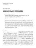
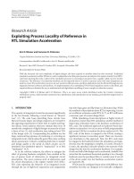
7.1. General Results. In Figure 1, the average sum rate, the
average worst-case delay, and the dispersion are shown for
the four studied schedulers. In Figure 1(a), the users are
symmetrically distributed, that is, c
= 1, whereas in Figure
1(b), the users are asymmetrically distributed according to
the model in (51)witht
= 0.2. The results in Figure 1
illustrate the following observations. The average sum rate
of MTS increases with more asymmetrically distributed
users(compareto(14)), while the average sum rate of
all three other schedulers decreases (compare to (15),
(18), and (20)). However, PFS outperforms ORS for the
symmetrical scenario, whereas it is the other way round
for the asymmetrical scenario. Another observation is that
the average worst-case delay is more differentiated than
the dispersion. This underlines that the average worst-
case delay is better suited for fairness analysis than the
JFI-based dispersion. Finally, the average worst-case delay
for the asymmetrical scenario of the PFS and ORS tends
to grow without bound. Therefore, taking the tradeoff
between fairness and average sum rate into account, the
PFS and ORS perform reasonable well. PFS is advantageous
in symmetric scenarios whereas ORS performs better in
asymmetric scenarios.
Scaling with number of users (symmetrical distribution)
2.5

3
3.5
4
4.5
5
5.5
Average sum rate (bpcu)
2 4 6 8 10 12 14 16 18 20
Number of users
RRS
MTS
PFS
ORS
(a)
Scaling with number of users (symmetrical distribution)
0
10
20
30
40
50
60
70
80
Average worst-case delay
2 4 6 8 10 12 14 16 18 20
Number of users
MTS
PFS
RRS

ORS
(b)
Figure 2: Average sum rate and worst-case delay versus number of
users for symmetrically distributed users.
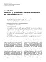
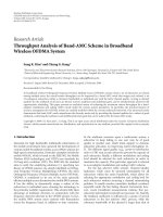
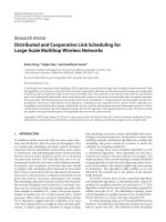
7.2. Scaling with Number of Users. In Figures (2)and(3),
we show the average performance of the four scheduling
algorithms for symmetrically distributed as well as asymmet-
rically distributed users. The derived scaling laws in (40)and
(41) are confirmed. The interesting observation is that for the
asymmetrical case, PFS outperforms OFS for a small number
of users, whereas it is the other way round for large number
of users.
The average worst case delay for MTS and PFS
increases with asymmetrical user distribution as predicted
in Theorem 5. As soon as a single c
k
approaches zero, the
average worst-case delay approaches infinity. The round-
based schedulers RRS and ORS are robust against the
asymmetrical user distribution.
The main observation in this section is that for practical
scenarios in which fairness is important as well as users are
randomly distributed within the cell, ORS clearly outper-
forms PFS. Note that the results presented here hold for a
10 EURASIP Journal on Wireless Communications and Networking
Scaling with number of users (assymetrical with t = 0.2)
2
2.5
3
3.5

4
4.5
5
5.5
6
Average sum rate (bpcu)
2 4 6 8 10 12 14 16 18 20
Number of users
RRS
MTS
PFS
ORS
(a)
Scaling with number of users (assymetrical t = 0.2)
0
10
20
30
40
50
60
70
80
Average worst-case delay
2 4 6 8 10 12 14 16 18 20
Number of users
RRS
MTS
PFS
ORS

(b)
Figure 3: Average sum rate and worst-case delay versus number of
users for asymmetrically distributed users.
static scenario in which we place the users only once inside
the cell and simulate the small-scale fading. Mobility as well
as traffic models is left for further research.
7.3. Multiple Antenna Case—OSTBC. The application of
OSTBC yields to a tradeoff between the code rate and the
number of degrees of freedom of the channel gain. The code
rate r
C
decreases with the number of antennas, whereas the
number of degrees of freedom of the χ
2
distributed channel
gain increases. For an OSTCB with n
T
transmit antennas, it
is shown in [35] that the maximum achievable code rate is
given by
r
C
(n
T
) =

n
T
+1


/2

+1
2

n
T
+1

/2

. (53)
7
7.5
8
8.5
9
9.5
Average sum rate (bpcu)
8
7654
Average worst-case delay
PFS
RRS
MTS
ORS
Figure 4: Average sum rate/worst-case delay tradeoff, n
T
=
{

1, 2}; K = 4; SNR = 20 dB.
The code rate r
C
(n
T
) starts at r
C
(1) = r
C
(2) = 1and
decreases to lim
n
T
→∞
r
C
(n
T
) = 1/2. Therefore, we restrict the
numerical simulations to the case n
T
= 2.
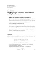
In Figure 4, the achievable average sum rate versus
average worst-case delay tradeoff is shown for a two antenna
BS with four users at SNR
= 20 dB for the four schedulers.
The PFS is operated at ten window length operating
points t
c
= 2

k
, k = 1, , 10. The RRS has lowest delay,
whereas the MTS has largest delay but best performance.
The closure of the convex hull of all operating points
gives the achievable sum rate/delay region. The dashed
line shows the single-antenna case. It can be observed
that two antennas increase average sum rate as well as
decrease the average worst-case delay significantly. Note that
no additional (spatial) feedback is required to achieve this
gain.
8. Conclusions
In this paper, we proposed an approach to analyze qualita-
tively the tradeoff between system throughput and fairness
in a multiuser multiple antenna downlink transmission
system. Four representative (three of them channel aware)
schedulers were studied for different user distributions
using majorization theory. The sum rate of MTS improves
with asymmetrical user distribution, whereas the sum rate
of all other schedulers improves with symmetrical user
distribution. MTS and RRS serve as upper and lower bounds
on throughput and lower and upper bounds on worst-
case delay, respectively. The throughput-delay tradeoff of
the four schedulers is characterized; if fairness as well as
performance is important, the optimal choice will depend
on the user distribution and the number of users. Finally, the
gain of using multiple antennas without increased feedback
overhead at the base station is illustrated.
EURASIP Journal on Wireless Communications and Networking 11
Appendices
A. Proof of Theorem 1

Proof. In the proof, we verify Schur’s condition directly.
Therefore, we need the first derivative of R
MT
sum
with respect
to c
1
and c
2
given as
∂R
MT
sum
∂c
1
=

∞
0
ρt
1+ρt
K

k=3

1 −
Γ

n
T

,

t/c
k

Γ

n
T


·

1 −
Γ

n
T
,

t/c
2

Γ

n
T


(t

n
T
−1
/c
1

c
2
1
Γ

n
T

exp

−
t
c
1

dt,
∂R
MT
sum
∂c
2
=

∞

0
ρt
1+ρt
K

k=3

1 −
Γ

n
T
,

t/c
k

Γ

n
T


·

1 −
Γ

n
T

,

t/c
1

Γ

n
T


(t
n
T
−1
/c
2

c
2
1
Γ

n
T

exp

−
t

c
2

dt.
(A.1)
Define the two functions
f (ρ, t, c)
=
ρt
1+ρt
K

k=3

1 −
Γ

n
T
,

t/c
k

Γ

n
T



,
g(t, c
1
, c
2
) =

1 −
Γ

n
T
,

t/c
2

Γ

n
T



t/c
1

n
T
−1

c
2
1
Γ

n
T

exp

−
t
c
1

−

1 −
Γ

n
T
,

t/c
1

Γ

n

T



t/c
2

n
T
−1
c
2
2
Γ

n
T

exp

−
t
c
2

,
(A.2)
in order to express the difference of the first derivatives of the
sumrateoftheMTSas
∂R

MT
sum
∂c
1
−
∂R
MT
sum
∂c
2
=

∞
0
f (ρ, t, c)g(t, c
1
, c
2
)dt. (A.3)
The following properties of the functions f and g are easily
verified; f is monotonic increasing from zero to one. The
function g is g(t
= 0) = 0, has one zero at t
∗
: g(t
∗
) = 0, and
is negative for all t<t
∗
and positive for all t>t

∗
. Therefore,
we can lower bound (A.3) by using the zero t
∗
as
∂R
MT
sum
∂c
1
−
∂R
MT
sum
∂c
2
≥ f (ρ, t
∗
, c)

∞
0
g

t, c
1
, c
2

dt. (A.4)

Finally, the integral in (A.4) can be computed in closed form

∞
0
g

t, c
1
, c
2

dt =
1
2
1
c
1
c
2
Γ

1+n
T

√
π
·

2
√

πΓ

n
T
+1

c
2
−c
1

+ Γ

n
T
+1/2

4
n
T

c
1
c
2

n
T
·


c
1
·
2
F
1

n
T
,2n
T
;1+n
T
; −

c
1
c
2

−
c
2
·
2
F
1

n
T

,2n
T
;1+n
T
; −

c
2
c
1

,
(A.5)
where
2
F
1
(a, b; c; z) is the Gauss hypergeometric function
[30, Chapter 15]. For single-antenna BS, we set n
T
= 1to
obtain
G

c
1
, c
2
,1


=
0, (A.6)
which is in perfect agreement with the result and its
proof in [28]. Since, the function G(c
1
, c
2
, n
T
) is monotonic
increasing with n
T
, this implies that
∂R
MT
sum
∂c
1
−
∂R
MT
sum
∂c
2
≥ f (ρ, t
∗
, c)G

c
1

, c
2
, n
T

≥
0, (A.7)
which verifies Schur’s condition for Schur convexity.
B. Proof of Theorem 4
Proof. The proof is similar to the proof in Appendix A.The
difference is that we have two sums in the integral instead
of the product. Starting from the representation in (10), the
difference of the first partial derivatives with respect to c
1
and
c
2
, respectively, is computed
∂R
OR
sum
∂c
1
=

∞
0
ρ
1+ρt
1

K
2
·
K

k=1

1 −

Γ

n
T
, t/c
1

/Γ

n
T

k
kt
n
T
exp

−
t/c
1


Γ

n
T

−
Γ

n
T
, t/c
1

c
n
T
+1
1
dt,
∂R
OR
sum
∂c
2
=

∞
0
ρ

1+ρt
1
K
2
·
K

k=1

1 −

Γ

n
T
, t/c
2

/Γ

n
T

k
kt
n
T
exp

−

t/c
2

Γ

n
T

−Γ

n
T
, t/c
2

c
n
T
+1
2
dt.
(B.1)
Define the two functions
φ(ρ, t)
=
ρ
1+ρt
,
γ


t, c
1
, c
2
, k, n
T

=

1 −

Γ

n
T
, t/c
1

/Γ

n
T

k
kt
n
T
exp

−

t/c
1

Γ

n
T

−
Γ

n
T
, t/c
1

c
n
T
+1
1
−

1 −

Γ(n
T
, t/c
2


/Γ

n
T

k
kt
n
T
exp

−
t/c
2

Γ

n
T

−
Γ

n
T
, t/c
2

c
n

T
+1
2
,
(B.2)
inordertorewritethedifference of the first derivatives as
Δ
=
∂R
OR
sum
∂c
1
−
∂R
OR
sum
∂c
2
=
1
K
2
K

k=1

∞
0
φ(ρ, t)γ


t, c
1
, c
2
, k, n
T

dt.
(B.3)
The properties of the functions φ and γ areasfollows.φ is
monotonic decreasing with respect to t,andγ has similar
properties as the function g in the proof in Appendix A.
12 EURASIP Journal on Wireless Communications and Networking
γ(t
= 0) = 0, it has on zero at t
∗
: g(t
∗
) = 0, it is negative for
all t<t
∗
and positive for all t>t
∗
. Therefore, we obtain an
upper bound on Δ in (B.3)as
Δ
≤
1
K

2
K

k=1
φ(ρ, t
∗
)

∞
0
γ

t, c
1
, c
2
, k, n
T

dt = 0, (B.4)
because

∞
0
γ(t, c
1
, c
2
, k, n
T

)dt = 0. This verifies Schur’s
condition for Schur concavity and completes the proof.
References
[1] R. Knopp and P. A. Humblet, “Information capacity and
power control in single-cell multiuser communications,” in
Proceedings of IEEE International Conference on Communica-
tions (ICC ’95), vol. 1, pp. 331–335, Seattle, Wash, USA, June
1995.
[2] D. Tse and P. Viswanath, Fundamentals of Wireless Communi-
cation, Cambridge University Press, Cambridge, UK, 2005.
[3] T. Issariyakul and E. Hossain, “ORCA-MRT: an optimization-
based approach for fair scheduling in multirate TDMA wire-
less networks,” IEEE Transactions on Wireless Communications,
vol. 4, no. 6, pp. 2823–2835, 2005.
[4] X. Wang, A. G. Marques, and G. B. Giannakis, “Power-
efficient resource allocation and quantization for TDMA
using adaptive transmission and limited-rate feedback,” IEEE
Transactions on Signal Processing, vol. 56, no. 9, pp. 4470–4485,
2008.
[5] F. Halsall, Data Communications, Computer Networks and
Open Systems, Electronic Systems Engineering, Addison-
Wesley, Reading, Mass, USA, 4th edition, 1996.
[6] L. Yang and M S. Alouini, “Performance analysis of multiuser
selection diversity,” IEEE Transactions on Vehicular Technology,
vol. 55, no. 6, pp. 1848–1861, 2006.
[7] S. S. Kulkarni and C. Rosenberg, “Opportunistic scheduling
policies for wireless systems with short term fairness con-
straints,” in Proceedings of IEEE Global Telecommunications
Conference (GLOBECOM ’03), vol. 1, pp. 533–537, San
Francisco, Calif, USA, December 2003.

[8] V. Hassel, G. E. Øien, and D. Gesbert, “Throughput guaran-
tees for wireless networks with opportunistic scheduling: a
comparative study,” IEEE Transactions on Wireless Communi-
cations, vol. 6, no. 12, pp. 4215–4220, 2007.
[9] G. Song and Y. Li, “Asymptotic throughput analysis for
channel-aware scheduling,” IEEE Transactions on Communi-
cations, vol. 54, no. 10, pp. 1827–1834, 2006.
[10] R. Jain, D. Chiu, and W. Hawe, “A quantitative measure of
fairness and discrimination for resource allocation in shared
computer systems,” Research Report TR-301, DEC, New York,
NY, USA, September 1984.
[11] R. Elliott, “A measure of fairness of service for scheduling algo-
rithms in multiuser systems,” in Proceedings of the Canadian
Conference on Electrical and Computer Engineering (CCECE
’02), vol. 3, pp. 1583–1588, Winnipeg, Canada, May 2002.
[12] M. Sharif and B. Hassibi, “Delay considerations for oppor-
tunistic scheduling in broadcast fading channels,” IEEE Trans-
actions on Wireless Communications, vol. 6, no. 9, pp. 3353–
3363, 2007.
[13] N. Golmie, Coexistence in Wireless Networks, Cambridge
University Press, Cambridge, UK, 2007.
[14] Z. Han and K. J. R. Liu, Resource Allocation for Wireless
Networks: Basics, Techniques, and Applications, Cambridge
University Press, Cambridge, UK, 2008.
[15] E. A. Jorswieck, A. Sezgin, and X. Zhang, “Framework
for analysis of opportunistic schedulers: average sum rate
vs. average fairness,” in Proceedings of the 4th Workshop
on Resource Allocation in Wireless Networks (RAWNET ’08),
Berlin, Germany, March 2008.
[16] A. Sezgin, E. Jorswieck, and M. Charafeddine, “Interaction

between scheduling and user locations in an OSTBC coded
downlink system,” in Proceedings of the 7th International ITG
Conference on Source and Channel Coding (SCC ’08),Ulm,
Germany, January 2008.
[17] S. M. Alamouti, “A simple transmit diversity technique for
wireless communications,” IEEE Journal on Selected Areas in
Communications, vol. 16, no. 8, pp. 1451–1458, 1998.
[18] V. Tarokh, H. Jafarkhani, and A. R. Calderbank, “Space-time
block codes from orthogonal designs,” IEEE Transactions on
Information Theory, vol. 45, no. 5, pp. 1456–1467, 1999.
[19] E. Jorswieck, B. Ottersten, A. Sezgin, and A. Paulraj, “Guar-
anteed performance region in fading orthogonal space-time
coded broadcast channels,” EURASIP Journal on Wireless
Communications and Networking, vol. 2008, Article ID 268979,
12 pages, 2008.
[20] A. Sezgin and E. Jorswieck, “On the performance of partial
feedback based orthogonal block coding,” in Proceedings of the
62nd IEEE Vehicular Technology Conference (VTC ’05), vol. 3,
pp. 1504–1508, Dallas, Tex, USA, September 2005.
[21] A. W. Marshall and I. Olkin, Inequalities: Theory of Majoriza-
tion and Its Application, vol. 143 of Mathematics in Science and
Engineering, Academic Press, New York, NY, USA, 1979.
[22]R.A.HornandC.R.Johnson,Matrix Analysis, Cambridge
University Press, Cambridge, UK, 1985.
[23] E. Jorswieck and H. Boche, “Majorization and matrix-
monotone functions in wireless communications,” Founda-
tions and Trends in Communications and Information Theory,
vol. 3, no. 6, pp. 553–701, 2006.
[24] A. Lozano, A. M. Tulino, and S. Verd
´

u, “High-SNR power
offset in multiantenna communication,” IEEE Transactions on
Information Theory, vol. 51, no. 12, pp. 4134–4151, 2005.
[25] C J. Chen and L C. Wang, “A unified capacity analysis for
wireless systems with joint multiuser scheduling and antenna
diversity in Nakagami fading channels,” IEEE Transactions on
Communications, vol. 54, no. 3, pp. 469–478, 2006.
[26] M. Johansson, “Diversity-enhanced equal access—
considerable throughput gains with 1-bit feedback,” in
Proceedings of the 5th IEEE Workshop on Signal Processing
Advances in Wireless Communications (SPAWC ’04), pp. 6–10,
Lisbon, Portugal, July 2004.
[27] V. Hassel, M. R. Hanssen, and G. E. Øien, “Spectral efficiency
and fairness for opportunistic round robin scheduling,” in
Proceedings of IEEE International Conference on Communica-
tions (ICC ’06), vol. 2, pp. 784–789, Istanbul, Turkey, July 2006.
[28] E. A. Jorswieck and H. Boche, “Throughput analysis of cellular
downlink with different types of channel state information,”
in Proceedings of IEEE International Conference on Communi-
cations (ICC ’06), vol. 4, pp. 1526–1531, Istanbul, Turkey, July
2006.
[29] D. J. Newman and L. Shepp, “The double dixie cup problem,”
The American Mathematical Monthly, vol. 67, no. 1, pp. 58–61,
1960.
[30] M. Abramowitz and I. A. Stegun, Handbook of Mathematical
Functions, Dover, New York, NY, USA, 1970.
[31] M. L. Clevenson and W. Watkins, “Majorization and the
birthday inequality,” Mathematics Magazine,vol.64,no.3,pp.
183–188, 1991.
EURASIP Journal on Wireless Communications and Networking 13

[32] E. A. Jorswieck, P. Svedman, and B. Ottersten, “Performance of
TDMA and SDMA based opportunistic beamforming,” IEEE
Transactions on Wireless Communications, vol. 7, no. 11, pp.
4058–4063, 2008.
[33] T. Bonald and A. Proutire, “On the traffic capacity of
cellular data networks,” in Proceedings of the 24th International
Conference on Thermoelectrics (ICT ’05), Clemson, SC, USA,
June 2005.
[34] E. A. Jorswieck and H. Boche, “Delay-limited capacity:
multiple antennas, moment constraints, and fading statistics,”
IEEE Transactions on Wireless Communications, vol. 6, no. 12,
pp. 4204–4208, 2007.
[35] X B. Liang, “Orthogonal designs with maximal rates,” IEEE
Transactions on Information Theory, vol. 49, no. 10, pp. 2468–
2503, 2003.