Báo cáo hóa học: " Research Article Modelling Transcriptional Regulation with a Mixture of Factor Analyzers and Variational Bayesian Expectation Maximization" doc

Hindawi Publishing Corporation
EURASIP Journal on Bioinformatics and Systems Biology
Volume 2009, Article ID 601068, 26 pages
doi:10.1155/2009/601068
Research Article
Modelling Transcriptional Regulation with a Mixture of Factor
Analyzers and Vari ational Bayesian Expectation Maximization
Kuang Lin and Dirk Husmeier
Biomathematic s & Statistics Scotland (BioSS), Edinburgh EH93JZ, UK
Correspondence should be addressed to Dirk Husmeier,
Received 2 December 2008; Accepted 27 February 2009
Recommended by Debashis Ghosh
Understanding the mechanisms of gene transcriptional regulation through analysis of high-throughput postgenomic data is one of
the central problems of computational systems biology. Various approaches have been proposed, but most of them fail to address
at least one of the following objectives: (1) allow for the fact that transcription factors are potentially subject to posttranscriptional
regulation; (2) allow for the fact that transcription factors cooperate as a functional complex in regulating gene expression, and
(3) provide a model and a learning algorithm with manageable computational complexity. The objective of the present study is
to propose and test a method that addresses these three issues. The model we employ is a mixture of factor analyzers, in which
the latent variables correspond to different transcription factors, grouped into complexes or modules. We pursue inference in
a Bayesian framework, using the Variational Bayesian Expectation Maximization (VBEM) algorithm for approximate inference
of the posterior distributions of the model parameters, and estimation of a lower bound on the marginal likelihood for model
selection. We have evaluated the performance of the proposed method on three criteria: activity profile reconstruction, gene
clustering, and network inference.
Copyright © 2009 K. Lin and D. Husmeier. This is an open access article distributed under the Creative Commons Attribution
License, which permits unrestricted use, distribution, and reproduction in any medium, provided the original work is properly
cited.
1. Introduction
Transcriptional gene regulation is a complex process that
utilizes a network of interactions. This process is primarily
controlled by diverse regulatory proteins called transcription
factors (TFs), which bind to specific DNA sequences and

thereby repress or initiate gene expression. Transcriptional
regulatory networks control the expression levels of thou-
sands of genes as part of diverse biological processes such
as the cell cycle, embryogenesis, host-pathogen interactions,
and circadian rhythms. Determining accurate models for TF-
genes regulatory interactions is thus an important challenge
of computational systems biology. Most recent studies of
transcriptional regulation can be placed broadly in one of
three categories.
Approaches in the first class attempt to build quantitative
models to associate gene expression levels, as typically
obtained from microarray experiments, with putative bind-
ing motifs on the gene promoter sequences. Bussemaker et al.
[1] and Conlon et al. [2] propose a linear regression model
for the dependence of the log gene expression ratio on the
presence of regulatory sequence motifs. Beer and Tavazoie
[3] cluster gene expression profiles in a preliminary data
analysis based on correlation, and then apply a Bayesian
network classifier to predict cluster membership from
sequence motifs. Phuong et al. [4] use multivariate decision
trees to find motif combinations that define homogeneous
groups of genes with similar expression profiles. Segal et al.
[5] cluster genes with a probabilistic generative model
that systematically integrates gene expression profiles with
regulatory sequence motifs.
A shortcoming of the methods in the first class is that
the activities of the TFs are not included in the model.
This limitation is addressed by models in the second class,
which predict gene expression levels from both binding
motifs on promoter sequences and the expression levels

of putative regulators. Middendorf et al. [6, 7] approach
this problem as a binary classification task to predict up-
and down-regulation of a gene from a combination of a
motif presence/absence indication and the discrete state of
2 EURASIP Journal on Bioinformatics and Systems Biology
Gene
expression
TF
(a)
Gene
expression
TF
module
TF
(b)
Figure 1: Transcriptional regulatory network. (a) A transcriptional regulatory network in the form of a bipartite graph, in which a small
number of transcription factors (TFs), represented by circles, regulate a large number of genes (represented by squares) by binding to
their promoter regions. The black lines in the square boxes indicate gene expression profiles, that is, gene expression values measured
under different experimental conditions or for different time points. The black lines in the circles represent TF activity profiles, that is,
the concentrations of the TF subpopulation capable of DNA binding. Note that these TF activity profiles are usually unobserved owing to
posttranslational modifications, and should hence be included as hidden or latent variables in the statistical model. (b) A more accurate
representation of transcriptional regulation that allows for the cooperation of several TFs forming functional complexes; this complex
formation is particularly common in higher eukaryotes.
a putative regulator. The bidimensional regression trees of
Ruan and Zhang [8] are based on a similar idea, but avoid
the information loss inherent in the binary gene expression
discretization.
Transcriptional regulation is influenced by TF activities,
that is the concentration of the TF subpopulation capa-
ble of DNA binding. The methods in the second class

approximate the activities of TFs by their gene expres-
sion levels. However, TFs are frequently subject to post-
translational modifications, which may affect their DNA
binding capability. Consequently, gene expression levels of
TFs contain only limited information about their actual
activities. The methods in the third class address this
shortcoming by treating TFs as latent or hidden components.
The regulatory system is modelled as a bipartite network,
as shown in Figure 1(a), in which high-dimensional output
data are driven by low-dimensional regulatory signals. The
high-dimensional output data correspond to the expression
levels of a large number of regulated genes. The regulators
correspond to a comparatively small number of TFs, whose
activities are unknown. Various authors have applied latent
variable models like principal component analysis (PCA),
factor analysis (FA), and independent component analysis
(ICA) to determine a low-dimensional representation of
high-dimensional gene expression profiles; for example, Ray-
chaudhuri et al. [9] and Liebermeister [10]. However, these
approaches provide only a phenomenological modelling of
the observed data, and the hidden components do not
correspond to identified TFs. Liao et al. [11]andKao
et al. [12] address this shortcoming by including partial
prior knowledge about TF-gene interactions, as obtained
from Chromatin Immunoprecipitation (ChIP) experiments
[13] or binding motif finding algorithms (e.g., Bailey and
Elkan [14]; Hughes et al. [15]). Their network component
analysis (NCA) is equivalent to a constrained maximum
likelihood procedure in the presence of Gaussian noise and
independent hidden components; the latter represent the

TF activities. A major limitation of NCA is the fact that
the constraints on the connectivity pattern of the bipartite
network are rigid, which does not allow for the noise
intrinsic to immunoprecipitation experiments or sequence
motif detection. Sabatti and James [16] and Sanguinetti
et al. [17] address this shortcoming by proposing an
approach based on Bayesian factor analysis, in which prior
knowledge about TF-gene interactions naturally enters the
model in the form of a prior distribution on the elements
of the loading matrix. Pournara and Wernisch [18]propose
an alternative approach based on maximum likelihood,
where the loading matrix is orthogonally rotated towards a
target matrix of a priori known TF-gene interactions. All
three approaches simultaneously reconstruct the structure
of the bipartite regulatory network—represented by the
loading matrix—and the TF activity profiles—represented
by the hidden factors—from gene expression data and
(noisy) prior knowledge about TF-gene interactions. In
a recent generalization of these approaches, Shi et al.
[19] have introduced a further latent variable to indicate
whether a TF is transcriptionally or posttranscriptionally
regulated.
Contrary to the methods in the first two classes, the
methods in the third class do not incorporate interaction
effects between TFs, though. This is a major limitation,
since especially in higher eukaryotes transcription factors
cooperate as a functional complex in regulating gene expres-
sion [20, 21]. Boulesteix and Strimmer [22] allow for this
complex formation by proposing a latent variable model in
which the latent components correspond to groups of TFs.

However, their partial-least squares (PLS) approach does
not provide a probabilistic model and hence, like NCA,
does not allow for the noise inherent in TF binding profiles
from immunoprecipitation experiments or sequence motif
detection schemes.
EURASIP Journal on Bioinformatics and Systems Biology 3
In the present paper we aim to combine the advantages of
the methods in the three classes summarized above. Like the
approaches in the third class, our method is a latent variable
model that allows for the fact that owing to post-translational
modifications the true TF activities are unknown. Similar to
the approaches of the first two classes, our model explicitly
incorporates interactions among TFs. Inspired by Boulesteix
and Strimmer [22], we aim to group individual TFs into
TF modules, as illustrated in Figure 1(b). To allow for the
noise inherent in both gene expression levels and TF binding
profiles, we use a proper probabilistic generative model, like
Sanguinetti et al. [17] and Sabatti and James [16]. Our work
is based on the work of Beal [23]. We apply a mixture of
factor analyzers model, in which each component of the
mixture corresponds to a TF complex composed of several
TFs. This approach allows for the fact that TFs are not
independent. By explicitly including this in our model we
would expect to end up with fewer parameters, and hence
more stable inference. To further improve the robustness of
this approach, we pursue inference in a Bayesian framework,
which includes a model selection scheme for estimating
the number of TF complexes. We systematically integrate
gene expression data and TF binding profiles, and treat
both as data. This appears methodologically more consistent

than the approach in Sanguinetti et al. [17] and Sabatti
and James [16], where TF binding data are treated as
prior knowledge. Our paper is organized as follows. In
Section 2 we review Bayesian factor analysis applied to
modelling transcriptional regulation. In Section 3 we discuss
how TF complexes and interaction effects among TFs can
be modelled with a mixture of factor analyzers. The data
used for the evaluation of the method are described in
Section 4. Section 5 provides three types of results related
to the reconstruction of the unknown TF activity profiles
are discussed in Section 5.1, gene clustering is discussed in
Section 5.2, and the reconstruction of the transcriptional
regulatory network is discussed in Section 5.3.Weconclude
our paper in Section 6 with a summary and a brief outlook
on future work.
2. Background
In this section, we will briefly review the application of
Bayesian factor analysis to transcriptional regulation. To
keep the notation simple, we use the same letter p(
·)for
every probability distribution, even though they might be
of different functional forms. The form of p(
·)willbecome
clear from its argument, with p(x)andp(y) denoting
different distributions (strictly speaking, this should be
written as p
x
(x)andp
y
(y)). Variational distributions will

be written as q(
·). We do not distinguish between random
variables and their realization in our notation. However, we
do distinguish between scalars and vectors/matrices, using
bold-face letters for the latter, and using the superscript “
”
to denote transposition.
Given the expression levels of N genes at the ith
experimental condition, the objective of factor analysis
(FA) is to model correlations in high-dimensional data
y
i
= (y
i1
, , y
iN
)

by correlations in a lower-dimensional
subspace of unobserved or latent vectors x
i
= (x
i1
, , x
iK
)

,
which are assumed to have a zero-mean, unit-variance
Gaussian distribution. The model assumes that the latent

vectors x
i
are linearly mapped into the high-dimensional
space via a so-called loading matrix Λ, then translated
by μ, and finally subjected to additive noise from a zero-
mean Gaussian distribution with diagonal covariance matrix
Ψ. Mathematically, this procedure can be summarized as
follows:
y
i
= Λx
i
+ μ + e
i
,
(1)
x
i
∼ N
(
·|0, I
)
; e
i
∼ N
(
·|0, Ψ
)
,(2)
where N (

·|a, B) denotes a multivariate Gaussian distribu-
tion with mean vector a and covariance matrix B,0isazero-
vector, and I denotes the identity matrix. This probabilistic
generative model was first proposed by Ghahramani and
Hinton [24]. Note that in the context of gene regulation,
the vector y
i
corresponds to the gene expression profile in
experimental condition i, the latent vector x
i
denotes the
(unknown) TF activities in the same experimental condition,
and the elements of the loading matrix Λ represent the
strengths of the interactions between the TFs and the
regulated genes. Integrating out the latent vectors x
i
,itcan
be shown (see, for instance, Nielsen [25]) that
p

y
i
| Λ, μ, Ψ

=

p

y
i

| x
i
, Λ, μ,Ψ

p
(
x
i
)
dx
i
= N

y
i
| μ, ΛΛ

+ Ψ

,
(3)
where, from (1)and(2)
p

y
i
| x
i
, Λ, μ,Ψ


=
N

y
i
| Λx
i
+ μ, Ψ

. (4)
The likelihood of the data D
={y
1
, , y
T
} ,whereT is the
number of experimental conditions or time points, is given
by
p

D | Λ, μ,Ψ

=
T

i=1
p

y
i

| Λ, μ, Ψ

=
T

i=1
N

y
i
| μ, ΛΛ

+ Ψ

.
(5)
One can then, in principle, estimate the parameters Λ, μ, Ψ
in a maximum likelihood sense, using for instance the EM
algorithm proposed in Ghahramani and Hinton [24]and
Nielsen [25]. However, the maximum likelihood configu-
ration is not uniquely determined owing to two intrinsic
identifiability problems. First, there is a scale identifiability
problem: multiplying the loading matrix Λ by some factor a
and dividing the latent variables x
i
by the same factor will
leave (1) invariant. Second, subjecting the latent variables
x
i
to an orthogonal transformation x

i
→ Ux
i
will leave
the covariance matrix in (3) invariant, since ΛU(ΛU)

=
ΛUU

Λ

= ΛΛ

. Pournara and Wernisch [18]dealwith
this invariance by applying a varimax transformation to
4 EURASIP Journal on Bioinformatics and Systems Biology
rotate the loading matrix Λ towards maximum sparsity. The
justification of this approach, which we investigated in our
empirical evaluation to be discussed in Section 5, is that
gene regulatory networks are usually sparsely connected,
rendering sparse loading matrices Λ biologically more plau-
sible. An alternative approach to deal with this invariance,
which also allows the systematic integration of biological
prior knowledge, is to adopt a Bayesian approach. Here,
the parameters θ
={Λ, μ, Ψ} are interpreted as random
variables, for which prior distributions are defined. While the
likelihood shows a ridge owing to the invariance discussed
above, the posterior distribution does not (unless the prior
is uninformative), which solves the identifiability problem.

The most straightforward approach, chosen for instance in
Nielsen [25], Ghahramani and Beal [26]andBeal[23], is a
set of spherical Gaussian distributions as a prior distribution
for the column vectors in Λ
= (λ
1
, , λ
K
), where K is the
number of latent factors:
p
(
Λ
| ν
)
=
K

i=1
p
(
λ
i
| ν
i
)
=
K

i=1

N

λ
i
| 0,
1
ν
i
I

(6)
and a conjugate prior on the hyperparameters ν
=
(ν
1
, , ν
K
) in the form of a gamma distribution; see (20).
This approach shrinks the elements of the loading matrix
Λ to zero and is therefore similar in spirit to the varimax
rotation mentioned above. A more sophisticated approach,
which allows a more explicit inclusion of biological prior
knowledge about TF-gene interactions, was proposed in
Sanguinetti et al. [17] and Sabatti and James [16], based
on the work of West [27]. The models differ in various
details, but the generic idea can be described as follows. The
loading matrix element Λ
gt
, which indicates the strength of
the regulatory interaction between TF t and gene g, has the

prior probability
p

Λ
gt

=

1 − π
gt

δ

Λ
gt

+ π
gt
N

Λ
gt
| 0, ν
−1

(7)
where δ(
·) is the unit point mass at zero (the delta
distribution), and π
gt

denotes the prior probability of Λ
gt
to be different from zero. The precision hyperparameter
ν is given a gamma distribution with hyperparameters a
∗
and b
∗
, Gamma(ν | a
∗
, b
∗
); see (20). For the practical
implementation, a set of binary auxiliary variables Z
gt
∈
{
0, 1} is introduced, which indicate the presence or absence
of an interaction:
p

Λ
gt
| Z
gt
= 0

=
δ

Λ

gt

,
p

Λ
gt
| Z
gt
= 1

=
N

Λ
gt
| 0, σ
2
λ

.
(8)
The prior probability on the matrix of auxiliary variables Z
is given by
p
(
Z
)
=


g

t
π
Z
gt
gt
(1 − π
gt
)
1−Z
gt
,(9)
where the values of π
gt
allow the inclusion of prior knowl-
edge about TF-gene regulatory interactions, as obtained,
for example, from immunoprecipitation experiments or
sequence motif finding algorithms.
The objective of Bayesian inference is to learn the
posterior distribution of the model parameters and latent
variables. Since this distribution does not have a closed form,
approximate procedures have to be adopted. Sabatti and
James [16] follow a Markov chain Monte Carlo (MCMC)
approach based on the collapsed Gibbs sampler. Here, each of
the parameters Λ and Ψ and latent variables X
= (x
1
, , x
T

)
and Z is sampled separately from a closed-form distribution
that depends on sufficient statistics defined by the other
parameters/latent variables, and the procedure is iterated
until some convergence criterion is met. Sanguinetti et al.
[17] follow an alternative approach based on Variational
Bayesian Expectation maximization (VBEM), where the
joint posterior distribution of the parameters and latent vari-
ables is approximated by a product of model distributions for
which closed-form solutions can be obtained; see Section A.1
of the appendix.
3. Method
The Bayesian FA models discussed in the previous section
aim to explain changes in gene expression levels from the
activities of TFs, modelled as the hidden factors or latent
variables x
i
. This does not allow for the fact that in eukaryotes
TFs usually work in cooperation and form complexes [20],
and that gene regulation should be addressed in terms of
cis-regulatory modules rather than individual TF-gene inter-
actions. In the present paper, we address this shortcoming
by applying a mixture of factor analyzers (MFAs) approach.
Probabilistic mixture models are discussed in [42,Chapter
9], and the application to factor analysis models is discussed,
for instance, in McLachlan et al. [28]. We used a slight
variation of the mixture of factor analyzers (MFAs) approach
proposed in Ghahramani and Beal [26]andBeal[23].
Each component of the mixture represents a TF complex.
TF complexes are assumed to bind to the gene promoters

competitively, that is, each gene is regulated by a single TF
complex. Hence, while a gene can be regulated by several
TFs, these TFs do not act individually, but exert a combined
effect on the regulated gene via the TF complex they form.
In terms of modelling, our approach results in a dimension
and complexity reduction similar to the partial least squares
method proposed in Boulesteix and Strimmer [22], with the
difference that the approach proposed in the present paper
has the well-known advantages of a probabilistic generative
model, like improved robustness to noise and the provision
of an objective score for model selection and inference.
Consider the mixture model
p

y
i
| π, Λ, μ, Ψ

=
S

s
i
=1
Pr
(
s
i
| π
)

p

y
i
| λ
s
i
, μ
s
i
, Ψ

, (10)
where s
i
∈{1, , S} is a discrete random variable that
indicates the component from which y
i
has been generated,
and each component probability density p(y
i
| λ
s
i
, μ
s
i
, Ψ)is
given by (3). Pr(s
i

| π) is a prior probability distribution
on the components, defined by the vector of component
EURASIP Journal on Bioinformatics and Systems Biology 5
π
μ
∗
e
, ν
∗
e
μ
∗
b
, ν
∗
b
α
∗
, m
∗
Ψ
b
Ψ
e
i = 1, , N
s
= 1, , S
x
i
s

i
y
b
i
y
e
i
ν
s
μ
s
b
λ
s
b
λ
s
e
μ
s
e
a
∗
, b
∗
Figure 2: Bayesian mix ture of factor analyzers (MFA) model applied to transcriptional regulation. The figure shows a probabilistic
independence graph of the Bayesian mixture of factor analyzers (MFA) model proposed in Section 3. Variables are represented by circles,
and hyperparameters are shown as square boxes in the graph. S components (factor analyzers), each with their own parameters λ
s
= [λ

s
e
, λ
s
b
]
and μ
s
= [μ
s
e
, μ
s
b
], are used to model the expression profiles y
e
i
and TF binding profiles y
b
i
of i = 1, , N genes. The factor loadings λ
s
have
a zero-mean Gaussian prior distribution, whose precision hyperparameters ν
s
are given a gamma distribution determined by a
∗
and b
∗
.

The analyzer displacements μ
s
e
and μ
s
b
have Gaussian priors determined by the hyperparameters {μ
∗
e
, ν
∗
e
} and {μ
∗
b
, ν
∗
b
},respectively.The
indicator variables s
i
∈{1, , S} select one out of S factor analyzers, and the associated latent variables or factors x
i
have normal prior
distributions. The indicator variables s
i
are given a multinomial distribution, whose parameter vector π, the so-called mixture proportions,
have a conjugate Dirichlet prior with hyperparameters α
∗
m

∗
. Ψ
e
and Ψ
b
are the diagonal covariance matrices of the Gaussian noise in
the expression and binding profiles, respectively. A dashed rectangle denotes a plate, that is an iid repetition over the genes i
= 1, ,N or
the mixture components s
= 1, ,S, respectively. The biological interpretation of the model is as follows. μ
s
b
represents the composition
of the sth transcriptional module, that is, it indicates which TFs bind cooperatively to the promoters of the regulated genes. λ
s
b
allows
for perturbations that result, for example, from the temporary inaccessibility of certain binding sites or a variability of the binding affinities
caused by external influences. μ
s
e
is the background gene expression profile. λ
s
e
represents the activity profile of the sth transcriptional module,
which modulates the expression levels of the regulated genes. x
i
describes the gene-specific susceptibility to transcriptional regulation, that is,
to what extent the expression of the ith gene is influenced by the binding of a transcriptional module to its promoter. A complete description
of the model can be found in Section 3.

proportions π = (π
1
, , π
S
)viaPr(s
i
| π) = π
s
i
.
The component proportions are given a conjugate prior
in the form of a symmetric Dirichlet distribution with
hyperparameter α
∗
m
∗
, m
∗
= (1/S, ,1/S), where
p
(
π
| α
∗
m
∗
)
= Dir
(
π | α

∗
m
∗
)
=
Γ
(
α
∗
)
Γ(α
∗
/S)
S
S

s=1
π
α
∗
/S−1
s
.
(11)
As discussed in Section 2,(10)offers a way to relax the
linearity constraint of FA by means of tiling the data
manifold. One approach would be for y
i
to represent
the vector of gene expression values under experimental

condition i, and each experimental condition to be assigned
to one of S classes. However, this method would not achieve
the grouping of genes according to transcriptional modules.
We therefore transpose the data matrix D
= (y
1
, , y
T
),
where T is the number of experimental conditions or time
points, to obtain the new representation D
= (y
1
, , y
N
),
where N is the number of genes, and y
i
denotes the T-
dimensional column vector with expression values for gene
i under all experimental conditions. As we will be using this
representation consistently in the remainder of the paper,
we will not make the transposition (D

) explicit in the
notation. Note that in this new representation, (10)provides
a natural way to assign genes to transcriptional modules,
represented by the various components of the mixture. Recall
that in (1), the dimension of the hidden factor vector x
i

reflects the number of TFs regulating the genes. In the
proposed MFA model, the hidden factors are related to
TF complexes. Since each gene is assumed to be regulated
by a single complex, as discussed above, the hidden factor
vector becomes a scalar: x
i
→ x
i
. The loading matrix
Λ in (1) becomes a vector of the same dimension as y
i
and represents the TF complex activity profile (covering
the experimental conditions or time points for which gene
expression values have been collected in y
i
). We write this
as Λ
= (λ
1
, , λ
s
i
, , λ
S
). Equations (1)and(2)thus
become:
y
i
= λ
s

i
x
i
+ μ
s
i
+ e
i
,
(12)
x
i
∼ N
(
·|0, 1
)
; e
i
∼ N
(
·|0, Ψ
)
(13)
in which Ψ defines a diagonal covariance matrix, as before.
6 EURASIP Journal on Bioinformatics and Systems Biology
This can be rewritten as:
p

y
i

| x
i
, λ
s
i
, μ
s
i
, Ψ

=
N

y
i
| λ
s
i
x
i
+ μ
s
i
, Ψ

. (14)
For (3)wenowget:
p

y

i
| λ
s
i
, μ
s
i
, Ψ

=

p

y
i
| x
i
, λ
s
i
, μ
s
i
, Ψ

p
(
x
i
)

dx
i
= N

y
i
| μ
s
i
, λ
s
i
[λ
s
i
]

+ Ψ

(15)
which completes the definition of (10). Recall that in (1),
the loading matrix Λ provides a mechanism for including
biological prior knowledge about TF-gene interactions; this
approach, which was pursued in Sabatti and James [16],
is affected by the mixture prior of (7)–(9). However, like
gene expression levels, indications about TF-gene interac-
tions are usually obtained from microarray-type experi-
ments (ChIP-on-chip immunoprecipitation experiments). It
appears methodologically somewhat inconsistent to treat
these two types of data differently, and to treat gene

expression levels as proper data, while treating TF binding
data as prior knowledge. In our approach, we therefore seek
to treat both types of data on an equal footing. Denote
by y
e
i
the expression profile of gene i, that is, the vector
containing the expression values of gene i for the selected
experimental conditions or time points. In other words: y
e
ij
is the expression level of gene i in experimental condition j
(or at time point j). Denote by y
b
i
the TF binding profile of
gene i. This is a vector indicating the binding affinities of a set
of TFs for gene i. Expressed differently, y
b
ij
is the measured
strength with which TF j binds to the promoter of gene i.
In our approach, we concatenate these vectors to obtain an
expanded column vector y
i
:
y
i
=


y
e
i
, y
b
i

:=


y
e
i


,

y
b
i




. (16)
In practice, gene expression and TF binding profiles will
usually be differently distributed. The former tend to be
approximately log-normally distributed, while for the latter
we tend to get P-values distributed in the interval [0, 1].
It will therefore be advisable to standardize both types of

data to Normal distributions. For gene expression values this
implies a transformation to log ratios (or, more accurately,
the application of the mapping discussed in Huber et al.
[29]). P-values are transformed via z
= Φ
−1
(1 − p), where
Φ is the cumulative distribution function of the standard
Normal distribution. If p is properly calculated as a genuine
P-value, then under the null hypothesis of no significant TF
binding, z will be normally distributed. The concatenation
expressed in (16) implies a corresponding concatenation of
the parameter vectors λ
s
i
and μ
s
i
:
λ
s
i
=

λ
s
i
e
, λ
s

i
b

, μ
s
i
=

μ
s
i
e
, μ
s
i
b

, (17)
and the hyperparameters:
diag
(
Ψ
)
=

diag
(
Ψ
e
)

,diag
(
Ψ
b
)

,
μ
∗
=

μ
∗
e
, μ
∗
b

, ν
∗
=

ν
∗
e
, ν
∗
b

,

(18)
where μ
∗
and ν
∗
define the prior distributions on the
parameters, as discussed below. The resulting model can
be interpreted as follows: μ
s
b
represents the composition of
the sth transcriptional module, that is, it indicates which
TFs bind cooperatively to the promoters of the regulated
genes. λ
s
b
allows for perturbations that result, for example,
from the temporary inaccessibility of certain binding sites
or a variability of the binding affinities caused by external
influences. μ
s
e
is the “background” gene expression profile.
λ
s
e
represents the activity profile of the sth transcriptional
module, which modulates the expression levels of the
regulated genes. x
i

describes the gene-specific susceptibility
to transcriptional regulation, that is, to what extent the
expression of the ith gene is influenced by the binding
of a transcriptional module to its promoter. Naturally,
this information is contained in the expression profiles y
e
i
and TF binding profiles y
b
i
of the genes that are (softly)
assigned to the s
i
th mixture component, while (12)and
(13) provide a mechanism to allow for the noise in the
data.
Here is an alternative interpretation of our model,
which is based on the assumption that a variation of gene
expression is brought about by different TFs binding in
different proportions to the promoter. In the ideal case,
genes with the same TFs binding in identical proportions
to the promoter should have identical gene expression
profiles; this is expressed in our model by μ
s
b
(the pro-
portions of TFs binding to the promoter), and μ
s
e
(the

“background” gene expression profile associated with the
idealized binding profile of the TFs). Obviously, this model
is oversimplified. There are two reasons why gene expression
profiles might deviate from this idealized profile. The first
reason is measurement errors and stochastic fluctuations
unrelated to the TFs. These influences are incorporated in
the additive term e
i
in (12).Thesecondreasonisvariations
in the TF binding affinities, their activities and binding
capabilities. These variations are captured by the vector λ
s
b
.
The changes in the way TFs bind to the promoter will
result in deviations of the gene expression profiles from
the idealized “background” distribution; these deviations are
defined by the vector λ
s
e
. We assume that if the deviation of
the TF binding profiles from the idealized binding profile
μ
s
b
is small, the deviation from the “background” gene
expression profile μ
s
e
will be small. Conversely, if the TFs

show a considerable deviation from the idealized binding
profile μ
s
b
, then the gene expression profile will show a
substantial deviation from the idealized expression profile μ
s
e
.
We therefore scale both λ
s
b
and λ
s
e
by the same gene-specific
factor x
i
; this enforces a hard association between the two
effects described above. Weakening this association would be
biologically more realistic, but at the expense of increased
model complexity.
EURASIP Journal on Bioinformatics and Systems Biology 7
To complete the specification of the model, we need
to define prior distributions for the various parameter
groups. In the present paper we follow Beal [23]and
impose prior distributions on all parameters that scale
with the complexity of the model, that is, the number
of mixture components S. These are the factor loadings
{λ

s
i
} and displacement vectors {μ
s
i
}. The idea is that the
proper Bayesian treatment, that is, the integration over
these parameters, is essential to prevent over-fitting. Since
the number of degrees of freedom in Ψ does not depend
on the complexity of the model, integrating over these
parameters is less critical. In the present approach we
therefore follow the simplification suggested in Beal [23]
and treat Ψ as a parameter group to be estimated by
maximization of F in (22), see (A.24), rather than a
random variable with its own prior distribution. Like in
(6), a hierarchical prior is used for the factor loadings Λ
=
(λ
1
, , λ
S
):
p
(
Λ
| ν
)
=
S


s=1
N

λ
s
| 0,
I
ν
s

(19)
with gamma distributions for the precision hyperparameters
ν
= (ν
1
, , ν
S
):
p
(
ν
| a
∗
, b
∗
)
=
S

s=1

Gamma
(
ν
s
| a
∗
, b
∗
)
=
[b
∗
]
a
∗
Γ
(
a
∗
)
S

s=1
[ν
s
]
a
∗
−1
e

−b
∗
ν
s
.
(20)
A Gaussian prior with mean μ
∗
and precision matrix
diag[ν
∗
] is placed on the factor analyzer displacements μ
s
:
p

μ
1
, , μ
S

=
S

s=1
N

μ
s
| μ

∗
, diag
[
ν
∗
]
−1

, (21)
where diag[
·] is a square matrix that has the vector ν
∗
in
its diagonal, and zeros everywhere else. The corresponding
probabilistic graphical model is shown in Figure 2.
The objective of Bayesian inference is to estimate the
posterior distribution of the parameters and the marginal
posterior probability of the model (i.e., the number of
components in the mixture). The two principled approaches
to this end are MCMC and VBEM. A sampling-based
approach based on MCMC has been proposed in Fokou
´
e
and Titterington [30]. A VBEM approach has been proposed
in Ghahramani and Beal [26]andBeal[23]. In the present
work, we follow the latter approach. As briefly reviewed
in the appendix, Section A.1, the VBEM approach is based
on the choice of a model distribution that factorizes into
separate distributions of the parameters and latent variables:
q(θ, x, s)

= q(θ)q(x, s), where x = (x
1
, , x
N
)ands =
(s
1
, , s
N
). Following Beal [23], we assume the further
factorization of the distribution of the parameters θ: q(θ)
=
q(π, ν, Λ, μ) = q(π)q(ν)q(Λ, μ), where μ = [μ
1
, , μ
S
]and
λ
= [λ
1
, , λ
S
]. In generalization of (A.1)and(A.2)we
can now derive the following lower bound on the marginal
likelihood L
= p(D | M):
L
≥

dπq

(
π
)
ln
p
(
π
| α
∗
, m
∗
)
q
(
π
)
+
S

s=1

dν
s
q
(
ν
s
)

ln

p
(
ν
s
| a
∗
, b
∗
)
q
(
ν
s
)
+

d

Λ
s
q


Λ
s

ln
p



Λ
s
| ν
s
, μ
∗
, ν
∗

q


Λ
s

⎤
⎦
+
N

i=1
S

s
i
=1
q
(
s
i

)


dπq
(
π
)
ln
p
(
s
i
| π
)
q
(
s
i
)
+

dx
i
q
(
x
i
| s
i
)

ln
p
(
x
i
)
q
(
x
i
| s
i
)
+

d

Λq


Λ


dx
i
q
(
x
i
| s

i
)
×lnp

y
i
| s
i
, x
i
,

Λ
s
i
, Ψ

≡
F

q
(
π
)
,

q
(
ν
s

)
, q


Λ
s

,

q
(
s
i
)
, q
(
x
i
| s
i
)

N
i
=1

S
s
=1
,

α
∗
m
∗
, a
∗
, b
∗
, μ
∗
, ν
∗
, Ψ, D

,
(22)
where

Λ
s
≡ [λ
s
, μ
s
], D ={y
1
, , y
N
}, and all other
symbols are defined in Figure 2 and in the text; see [23,

equation (4.29)]. The variational E- and M-steps of the
VBEM algorithm are derived as in Section A.1 by setting
to zero the functional derivatives of F with respect to
the different (hyper-)parameters and latent variables under
consideration of possible normalization constraints, along
the line of (A.4)–(A.7). The derivations can be found in
Beal [23]. A summary of the update equations is provided in
the appendix, Section A.2. The various (hyper-)parameters
and latent variables are updated according to these equations
iteratively, assuming the variational distributions q(
·) for the
other (hyper-)parameters and latent variables are fixed. The
algorithm is iterated until a stationary point of F is reached.
The final issue to address is model selection, that is,
selecting the number of mixture components S. Following
Beal [23], we have not placed a prior distribution on S,but
instead have placed a symmetric Dirichlet prior over the
mixture proportions π;see(11). Equation (22)providesa
lower bound on the marginal likelihood L
= p(D | M),
where the model M is defined by the number of mixture
components S. In order to navigate in the space of different
model complexities, we use the scheme of birth and death
moves proposed in Beal [23]. This scheme can be seen as
the VBEM equivalent to reversible jump MCMC [31]. Via
a birth or a death move, a component is removed from or
introduced into the mixture model, respectively. The VBEM
algorithm, outlined in the present section and stated in more
detail in the appendix, Section A.2, is then applied until
a measure of convergence is reached. On convergence, the

move is accepted if F of (22) has increased, and rejected
8 EURASIP Journal on Bioinformatics and Systems Biology
Activity profiles
10 20 30 40
−2
0
2
10 20 30 40
−2
0
2
10 20 30 40
−2
0
2
10 20 30 40
−2
0
2
10 20 30 40
−2
0
2
10 20 30 40
−2
0
2
(a)
Expression profiles set 1
10 20 30 40

−4
−2
0
2
4
10 20 30 40
−4
−2
0
2
4
10 20 30 40
−4
−2
0
2
4
10 20 30 40
−4
−2
0
2
4
10 20 30 40
−4
−2
0
2
4
10 20 30 40

−4
−2
0
2
4
(b)
Expression profiles set 2
10 20 30 40
−4
−2
0
2
4
10 20 30 40
−4
−2
0
2
4
10 20 30 40
−4
−2
0
2
4
10 20 30 40
−4
−2
0
2

4
10 20 30 40
−4
−2
0
2
4
10 20 30 40
−4
−2
0
2
4
(c)
Expression profiles set 3
10 20 30 40
−4
−2
0
2
4
10 20 30 40
−4
−2
0
2
4
10 20 30 40
−4
−2

0
2
4
10 20 30 40
−4
−2
0
2
4
10 20 30 40
−4
−2
0
2
4
10 20 30 40
−4
−2
0
2
4
(d)
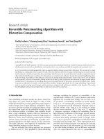
Figure 3: Simulated TF activity and expression profiles. (a) Simulated activity profiles of six hypothetical TF modules. The other panels show
simulated expression profiles of the genes regulated by the corresponding TF module (in the same row). From left to right, the three sets have
the corresponding observational noise levels of N (0, 0.25), N (0, 0.5) and N (0, 1). The vertical axes show the activity levels (a) or relative
log gene expression ratios (other panels), respectively, which are plotted against 40 hypothetical experiments or time points, represented by
the horizontal axes.
otherwise. Another birth/death proposal is then made, and
the procedure is repeated until no further proposals are
accepted. Further details of this birth/death scheme can be

found in Beal [23]. Note that these birth and death moves
also help avoid local maxima in F , in a similar manner as
discussed in Ueda et al. [32].
4. Data
We tested the performance of the proposed method on both
simulated and real gene expression and TF binding data.
The first approach has the advantage that the regulatory
network structure and the activities of the TF complexes are
known, which allows us to assess the prediction performance
of the model against a known gold standard. However, the
data generation mechanism is an idealized simplification
of real biological processes. We therefore also tested the
model on gene expression data and TF binding profiles from
Saccharomyces cerevisiae. Although S. cere visiae has been
widely used as a model organism in computational biology,
we still lack any reliable gold standard for the underlying
regulatory network, and therefore need to use alternative
evaluation criteria, based on out-of-sample performance. We
will describe the data sets in the present section, and discuss
the evaluation criteria together with the results in Section 5.
4.1. Synthetic Gene Expression and TF Binding Data. We
generated synthetic data to simulate both the processes of
transcriptional regulation as well as noisy data acquisition.
We started from the activities of the TF protein complexes
that regulate the genes by binding to their promoters. Note
that owing to post-translational modifications these activ-
ities are usually not amenable to microarray experiments
and therefore remain hidden. The advantage of the synthetic
data is that we can assess to what extent these activities can
be reconstructed from the gene expression profiles of the

regulated genes.
Figure 3(a) shows the activity profiles λ
s
, s = 1, ,6,of
6 TF modules for 40 hypothetical experimental conditions
or time points. Gene expression profiles (by gene expression
profile we mean the vector of log gene expression ratios with
respect to a control) y
i
were given by
y
i
= A
i
λ
s
+ e
i
, (23)
where A
i
∼ N (0,1) represents stochastic fluctuations and
dynamic noise intrinsic to the biological system, and e
i
EURASIP Journal on Bioinformatics and Systems Biology 9
10
20
30
40
50

60
70
80
90
246
Module connectivity
(a)
10
20
30
40
50
60
70
80
90
2468
TF binding
(b)
10
20
30
40
50
60
70
80
90
2468
Binding set 1

(c)
10
20
30
40
50
60
70
80
90
2468
Binding set 2
(d)
Figure 4: Simulated TF binding data. The figure shows simulated TF binding data. The vertical axis in each subfigure represents the 90 genes
involved in the regulatory network. From left to right: (a) The binary matrix of connectivity between the 6 TF modules (horizontal axis)
and the 90 genes, where black entries represent connections. Each module is composed of one or several TFs. (b) The real binding matrix
between TFs (horizontal axis) and genes (vertical axis), with black entries indicating binding. (c), (d) The noisy binding data sets used in the
synthetic study, with darker entries indicating higher values. Details can be found in Section 4.1.
represents observational noise introduced by measurement
errors. Here, I is the unit matrix. The expression profiles of
90 genes generated from (23) are shown in the right panels
of Figure 3. The algorithms were tested with expression
profile sets of three different noise levels: e
i
∼ N (0,0.25I),
N (0, 0.5I)orN (0, I). They were also tested with expression
profile sets of different lengths (numbers of time points or
experimental conditions). The first 10, 20 or 40 time points
were used.
Here we have assumed that each gene is regulated by

a single TF complex. Note, however, that an individual TF
can be involved in more than one TF module and therefore
contribute to the regulation of different subsets of genes, as
illustrated in Figure 1.RecallthatTFmodulesareprotein
complexes composed of various TFs. In practice, we usually
have only noisy indications about protein complex forma-
tions (e.g., from yeast 2-hybrid assays), and binding data
are usually available for individual TFs (from binding motif
similarity scores or immunoprecipitation experiments). In
our simulation experiment we therefore assumed that the
composition of the TF complexes was unknown, and that
noisy binding data were available for individual TFs, as
described shortly.
To group the TFs into modules when designing the
synthetic TF binding set, we followed Guelzim et al. [33]and
modelled the in-degree with an exponential distribution, and
the out-degree with a power-law distribution. In particular,
we chose the power-law distribution of P(k)
= 2k
−1
for
the out-degree. The in-degree followed the exponential
distribution of P(k)
= 102e
−0.69k
. The results are shown in
Figure 5. In the binding matrix, 9 TFs are connected to 90
genes via 142 edges, as shown in Figure 4(b).
In the real world, TF binding data—whether obtained
from gene upstream sequences via a motif search or from

immunoprecipitation experiments—are not free of errors,
and we therefore modelled two noise scenarios for two
different data formats. In the first TF binding set, the non-
binding elements were sampled from the beta distribution
beta(2, 4) and the binding elements from beta(4, 2). For the
second TF binding set, we chose beta(2, 10) and beta(10,2)
correspondingly. The resulting TF binding patterns are
shown in Figures 4(c), 4(d).
4.2. Gene Expression and TF Binding Data From Yeast. For
evaluating the inference of transcriptional regulation in
real organisms, we chose gene expression and TF binding
data from the widely used model organism Saccharomyces
cerevisiae (baker’s yeast). For the clustering experiments, we
combined ChIP-chip binding data of 113 TFs from Lee et al.
[34] with two different microarray gene expression data sets.
From the Spellman set [35], the expression levels of 3638
genes at 24 time points were used. From the Gasch set [36],
the expression values of 1993 genes at 173 time points were
taken. For evaluating the regulatory network reconstruction,
we used the gene expression data from Mnaimneh et al. [37]
and the TF binding profiles from YeastTract [38]. YeastTract
provides a comprehensive database of transcriptional regu-
latory associations in S. cerevisiae, and is publicly available
from />10 EURASIP Journal on Bioinformatics and Systems Biology
52
42
32
22
12
Number of regulated genes

123
In-degree
In-degree distribution
(a)
10
0
10
−1
Number of TFs
10
0
10
1
Out-degree
Out-degree distribution
(b)
Figure 5: In- and out-degree distributions of the simulated TF binding data. (a) The arriving connectivity distribution (in-degree distribution).
The number of genes regulated by k TFs follows an exponential distribution of P(k)
= 102e
−0.69k
for in-degree k. (b) The departing
connectivity distribution (out-degree distribution). The number of TFs per k follows the power-law distribution of P(k)
= 2k
−1
for out-
degree k. Note that an exponential distribution is indicated by a linear relationship between P(k)andk in a log-linear representation (a),
whereas a distribution consistent with the power law is indicated by a linear dependence between P(k)andk in a double logarithmic
representation (b).
included the expression levels of 5464 genes under 214
experimental conditions and binary TF binding patterns

associating these genes with 169 TFs.
5. Results and Discussion
We have evaluated the performance of the proposed method
on three criteria: activity profile reconstruction, gene clus-
tering, and network inference. The objective of the first
criterion, discussed in Section 5.1, is to assess whether the
activity profiles of the transcriptional regulatory modules can
be reconstructed from the gene expression data. The second
criterion, discussed in Section 5.2, tests whether the method
can discover biologically meaningful groupings of genes.
The third criterion, discussed in Section 5.3, addresses the
question of whether the proposed scheme can make a useful
contribution to computational systems biology, where one is
interested in the reconstruction of regulatory networks from
diverse sources of postgenomic data. We have compared
the proposed MFA-VBEM approach with various alternative
methods: the partial least squares approach proposed of
Boulesteix and Strimmer [22], maximum likelihood factor
analysis, effected with the EM algorithm of Ghahramani
and Hinton [24], and Bayesian factor analysis, using the
Gibbs sampling approach of Sabatti and James [16]. We did
not include network component analysis (NCA), introduced
by Liao et al. [11], in our comparison. NCA effectively
solves a constrained optimization problem, which only has
a solution if the following three criteria are satisfied: (i) the
connectivity matrix Λ must have full-column rank; (ii) each
column of Λ must have at least K
− 1zeros,whereK is the
number of latent nodes; (iii) the signal matrix X must have
full rank. These restrictions also apply to the more recent

algorithmic improvement proposed in Chang et al. [40].
These regularity conditions were not met by our data. In
particular, the absence of zeros in our connectivity matrices
violated condition (ii), causing the NCA algorithm to abort
with an error. An overview of the methods included in our
comparative evaluation study is provided in Tabl e 1.
5.1. Activity Profile Reconstruction. Since TF activity profiles
are not available for real data, we used the synthetic
data of Section 4.1 to evaluate the profile reconstruction
performance of the model. We have compared the proposed
MFA-VBEM model with the partial least-squares (PLS)
approach of Boulesteix and Strimmer [22], and with the
Bayesian factor analysis model using Gibbs sampling (BFA-
Gibbs), as proposed in Sabatti and James [16].
The PLS approach of Boulesteix and Strimmer [22]isfor-
mally equivalent to the FA model of equation (1). However,
the N-by-M loading matrix Λ, which linearly maps M latent
variables onto N genes, is decomposed into two matrices: an
N-by-K matrix describing the interactions between K TFs
and N genes, and an K-by-M matrix defining how the TFs
interact to form modules; see Figure 1(b). The elements of
the first matrix are fixed, taken from TF binding data (e.g.,
immunoprecipitation experiments or binding motifs). In the
present example, the binding matrices of Figures 4(c), 4(d)
EURASIP Journal on Bioinformatics and Systems Biology 11
Table 1: Overv iew of methods. An overview of the methods compared in our study with a brief description of how the TF regulatory network
was obtained.
PLS
The partial least squares approach proposed by Boulesteix and Strimmer [22], using the software provided by the
authors. Note that the method treats TF-gene interactions as fixed constants that cannot be changed in light of the

gene expression data. Hence, this approach cannot be used for network reconstruction and was only applied for
reconstructing the TF activity profiles.
FA
Maximum likelihood factor analysis, effected with the EM algorithm of Ghahramani and Hinton [24] and a subsequent
varimax rotation [39] of the loading matrix towards maximum sparsity, as proposed in Pournara and Wernisch [18].
BFA-Gibbs
Bayesian factor analysis of Sabatti and James [16], trained with Gibbs sampling. The TF regulatory network is obtained
from the posterior expected loading matrix via (A.32) and (A.35).
MFA-VBEM
The proposed mixture of factor analyzers model, shown in Figure 2 and discussed in Section 3, trained with variational
Bayesian Expectation Maximization. The approach is based on the work of Beal [23], with the extension described in
the text. The TF regulatory network is obtained from (24) and (25) for the curation and prediction tasks, respectively.
Table 2: Reconstruction of TF complex activity profiles. The mean
absolute correlation coefficient between the true and inferred
activity profiles, averaged over the 6 synthetic activity profiles of
Figure 3. N1, N2 and N3 refer to the three noise levels of e
i
∼
N (0, 0.25I), N (0, 0.5I)andN (0, I).L1,L2,andL3refertothe
expression profile lengths being 10, 20 and 40. B1 and B2 refer to
the two different binding data sets with different levels of noise.
Details are described in Section 4.1. Three methods have been
compared: the partial least squares (PLSs) approach of Boulesteix
and Strimmer [22]; the Bayesian factor analysis (BFA) model with
Gibbs sampling, as proposed in Sabatti and James [16]; and the
MFA model trained with VBEM, as described in Section 3.
Method B1 N1 N2 N3
PLS
L1
0.52 0.53 0.52

BFA 0.87 0.69 0.76
MFA 0.77 0.80 0.73
PLS
L2
0.52 0.52 0.52
BFA 0.84 0.68 0.59
MFA 0.89 0.71 0.60
PLS
L3
0.53 0.52 0.52
BFA 0.90 0.75 0.56
MFA 0.94 0.87 0.40
Method B2 N1 N2 N3
PLS
L1
0.53 0.52 0.52
BFA 0.92 0.89 0.78
MFA 0.88 0.83 0.71
PLS
L2
0.52 0.51 0.52
BFA 0.83 0.72 0.72
MFA 0.95 0.85 0.71
PLS
L3
0.52 0.51 0.52
BFA 0.90 0.73 0.67
MFA 0.98 0.94 0.63
were used. The elements of the second matrix are optimized
so as to minimize the sum-of-squares deviation between the

measured and reconstructed gene expression profiles subject
to an orthogonality constraint for the latent profiles. These
latent profiles are the predicted activity profiles of the TF
modules. A cross-validation approach can in principle be
used to optimize the number of TF modules M.However,
for ease of comparability of the reconstructed activity profiles
with those obtained with the other methods we set M to
the correct number of TF modules: M
= 6. We carried out
the evaluation using the software provided in Boulesteix and
Strimmer [22], using the default parameters.
The BFA-Gibbs method of Sabatti and James [16]
corresponds to a Bayesian FA model with a mixture prior
on the elements of the loading matrix Λ, which incorporates
the information from immunoprecipitation experiments or
binding motif search algorithms. In other words, the TF
binding data, which in the present evaluation were the
binding matrices of Figure 4, enter the model via the prior
on Λ, using (7)–(9). We sampled all parameters with the
Gibbs sampling method of Sabatti and James [16], using the
authors’ programs, and applying standard diagnostic tools
[41] to test for convergence of the Markov chains. The pre-
dicted activity profiles are the posterior averages of the latent
factor profiles, computed from (4) in Sabatti and James [16].
For the proposed MFA-VBEM model, the activity profile
of the sth TF module is given by
λ
s
e
, the posterior average

of λ
s
e
,whereλ
s
= [λ
s
e
, λ
s
b
] is the loading vector associated
with the sth module, and the posterior average
λ
s
is obtained
with the VBEM algorithm, using (A.17). The birth and death
moves of the VBEM scheme, explained in Section 3,allow
an estimation of the marginal posterior probability of the
number of TFs, M, which was found to peak at the correct
value of M
= 6. For a comparison with the alternative
approaches, the simulations were repeated with the number
of modules fixed at this value.
Ta ble 2 shows a comparison of the reconstruction accu-
racy in terms of the mean absolute Pearson correlation
between the true and estimated TF module activity profiles.
It is seen that BFA-Gibbs and the proposed MFA-VBEM
scheme consistently outperform PLS. The comparatively
poor performance of PLS, which has been independently

reported in Pournara and Wernisch [18], is a consequence
of the fact that PLS lacks any mechanism to deal with the
noise inherent in the TF binding profiles. In other words,
the noisy TF binding data of Figure 4 are taken as true fixed
TF-gene interactions, and there is no mechanism to adjust
them in light of the gene expression data. This shortcoming is
addressed by BFA-Gibbs and MFA-VBEM, which both allow
for the noise inherent in the TF binding data.
12 EURASIP Journal on Bioinformatics and Systems Biology
A comparison between BFA-Gibbs and MFA-VBEM
shows that BFA-Gibbs tends to outperform MFA-VBEM
when the expression profiles are short (length L1) or when
the noise level is high (N3). This could be a consequence of
the different inference schemes (“VBEM” versus “Gibbs”).
Short expression profiles and high noise levels lead to
diffuse posterior distributions of the parameters. Variational
learning—as opposed to Gibbs sampling—is known to lead
to a systematic underestimation of the posterior variation
[42], which could be a disadvantage here. However, MFA-
VBEM consistently outperforms BFA-Gibbs on the longer
expression profiles with lengths L2 and L3, and the lower
noise levels N1 and N2. We would argue that this improve-
ment in the performance is a consequence of the more
parsimonious model (“MFA”) that results when allowing for
the fact that TFs are non-independent, which leads to greater
robustness of inference and reduced susceptibility to over-
fitting.
5.2. Gene Clustering. Following up on the seminal work
of Eisen et al. [45], there has been considerable interest
in clustering genes based on their expression patterns. The

premise is based on the guilt-by-association hypothesis,
according to which similarity in the expression profiles might
be indicative of related biological functions. Although the
main purpose of the proposed MFA-VBEM method is not
one of clustering, it is straightforward to apply it to this
end by using the model mixture proportions q(s
i
), which are
obtained from the VBEM scheme via (A.22), as indicators
of class membership. A convenient feature of the MFA-
VBEM scheme is the fact that the number of clusters is
identical to the number of mixture components in the model.
This number is automatically inferred from the data using
the model selection scheme based on birth-death moves,
as described in Section 3. MFA-VBEM also allows for a
straightforward integration of gene expression profiles with
TF binding data.
We applied the MFA-VBEM method to the gene expres-
sion and TF binding data of S. cerevisiae, described in
Section 4.2. For comparison, we also applied two standard
clustering algorithms: K-means and hierarchical agglom-
erative average linkage clustering (see, e.g., Hastie et al.
[46]). We used the implementation of these two algorithms
in the Bioinformatics Toolbox of MATLAB (version 7.3.0),
using default parameters and the default distance measure
of 1 minus the absolute Pearson correlation coefficient. Five
randomly chosen initial starting points were chosen for
each application of K-means, and the most compact cluster
formation found was recorded. For hierarchical clustering,
we cut the dendrogram at such a distant from the root

that the number of resulting clusters equalled the number
of clusters used for MFA-VBEM and K-means. Note that
unlike the proposed MFA-VBEM approach, K-means and
average linkage clustering do not infer the number of clusters
automatically from the data. To ensure comparability of the
results we therefore set the number of clusters to be identical
to the number of mixture components inferred with the
MFA-VBEM method. We further included COSA [43]asa
more advanced clustering algorithm in our comparison. The
idea of clustering objects on subsets of attributes (COSA) is
to detect subgroups of objects that preferentially cluster on
subsets of the attribute variables rather than on all of them
simultaneously. The relevant attribute subsets for each indi-
vidual cluster can be different or partially overlap with other
clusters. The attribute subsets are automatically selected by
the algorithm via a weighting scheme that attempts to trade
off two effects: (1) the objective to identify homogeneous and
coherent clusters, and (2) the influence of an entropic regu-
larization term that penalizes small subset sizes. In our study,
we used the R program written by the authors, which is avail-
able from />∼jhf/COSA.html,
using the default settings of the parameters. Clusters were
obtained from the dendrogram in the same way as for
hierarchical agglomerative average linkage clustering, subject
to the constraint of having at least three genes in a cluster.
Finally, we included Plaid model clustering [44]inour
comparative evaluation study. Plaid model clustering is a
non-mutually exclusive clustering approach, which allows a
gene to have different cluster memberships. For the practical
computation we used the Plaid (TM) software copyrighted

by Stanford University, which is freely available from the fol-
lowing website: />∼owen/plaid/.
In order to evaluate the predicted clusters with respect
to their biological plausibility, we tested them for significant
enrichment of gene ontology (GO) annotations. To this
end, we used the GO terms from the Saccharomyces
genome database (SGD), which are publicly available from
We assessed the enrichment
for annotated GO terms in a given gene cluster with the
program Ontologizer [47], using the default parameters.
Given a population of genes with associated GO terms,
Ontologizer associates each GO term with a P-value. To
correct for multiple testing, we controlled the family-wise
type-I error conservatively with the Bonferroni correction,
using a standard threshold at the 5% significance level. We
called a gene cluster “biologically meaningful” if it contained
at least one significantly enriched GO term. We restricted this
analysis to specific GO terms, as generic and non-biologically
informative GO terms often tend to show a statistically
significant enrichment. Following a recommendation made
by one of the referees, we defined GO terms that were four
or less levels from the roots of the hierarchy defined in the
gene ontology (version February 29, 2008) as generic, and
discarded them from the subsequent analysis.
The results are shown in Ta bl e 3, which displays the
number of biologically meaningful clusters (in Column 3)
and the number of genes contained in them (Column 5).
On the expression data, the proposed MFA-VBEM approach
compares favorably with the competing methods and con-
sistently shows the best performance. When combining gene

expression data and TF binding profiles, MFA-VBEM consis-
tently outperforms all other methods: a higher proportion of
clusters is found to contain significantly enriched GO terms,
and more genes are contained in these clusters. This is a
demonstration of the robustness of MFA-VBEM in dealing
with a certain violation of the distributional assumptions
of the model; as a consequence of a thresholding operation
EURASIP Journal on Bioinformatics and Systems Biology 13
Table 3: Enrichment for GO terms in predicted gene clusters. The table shows the enrichment for known gene ontology (GO) terms in clusters
predicted with different clustering algorithms from different data sets. Five clustering algorithms were compared: hierarchical agglomerative
average linkage clustering, K-means, COSA [43], Plaid models [44], and the proposed MFA-VBEM scheme. The algorithms were applied
to a combination of different microarray gene expression data. For the proposed MFA-VBEM algorithm, we additionally included the
TF binding profiles of [34]. Clusters with significantly enriched GO terms (at the 5% significance level) are referred to as “biologically
meaningful clusters”. The number of genes in these clusters is shown in the rightmost column.
Data Clusters
Biologically
meaningful clusters
Genes
Genes in biologically
meaningful clusters
Average linkage
[35], E 48
10
3638
1483
[36], E 25
7
1993
1092
[35], E+B 30

8
3638
1148
[36], E+B 17
4
1993
703
K-means
[35], E 48
18
3638
1847
[36], E 25
12
1993
987
[35], E+B 30
13
3638
1337
[36], E+B 17
9
1993
884
COSA
[35], E 48
7
3638
1155
[36], E 25

8
1993
748
[35], E+B 30
10
3638
240
[36], E+B 17
4
1993
16
Plaid
[35], E 48
19
3638
1812
[36], E 25
10
1993
770
[35], E+B 30
11
3638
626
[36], E+B 17
9
1993
636
MFA-VBEM
[35], E 48

20
3638
2415
[36], E 25
16
1993
1278
[35], E+B 30
17
3638
2996
[36], E+B 17
14
1993
1645
E: clustering based on gene expression data only; E+B: clusters obtained from both gene expression and TF binding data.
applied to the experimentally obtained TF binding affinities,
the TF binding profiles extracted from YeastTract [38]are
binary rather than Gaussian distributed.
Interestingly, COSA shows a particularly poor perfor-
mance on the combined gene expression and TF binding
data. This can be explained as follows. The TF binding pro-
files extracted from YeastTract [38] are binary vectors, and
some TFs bind to several genes. The affected genes will have
identical (or very similar) binary profiles when restricted to
the respective TFs. With its inherent tendency to cluster on
subsets of attributes, COSA will group together genes that
happen to have similar binary entries for a small number of
TFs. This leads to the formation of many small clusters. These
clusters are not necessarily biologically meaningful, since

complementary information from the expression profiles
and other TFs has effectively been discarded.
It is also interesting to observe that the inclusion of
binding data occasionally deteriorates the performance of
K-means and hierarchical agglomerative clustering. This
deterioration is a consequence of the different nature of the
TF binding and gene expression profiles. While the former
are binary and hence nonnegative, the log gene expression
ratios my vary in sign. This renders the approach of combin-
ing them in a monolithic block suboptimal, as coregulated
genes may have anticorrelated expression profiles and
positively correlated TF binding patterns. Avoiding this
potential conflict by taking the modulus of the expression
profiles is no solution, as the resulting information loss was
found to lead to a deterioration of the clustering results. The
proposed MFA-VBEM model, on the other hand, uses the
extra flexibility that the model provides via the factor loading
vector λ
s
and the factor mean vector μ
s
(see Figure 2)toover-
come this problem. This suggests that MFA-VBEM provides
the right degree of flexibility as a compromise between the
rigidness of K-means and hierarchical agglomerative average
linkage clustering, and the over-flexible subset selection of
COSA. The consequence is an improvement in the biological
plausibility of the inferred gene clusters, as seen from Ta ble 3.
14 EURASIP Journal on Bioinformatics and Systems Biology
5.3. Regulatory Network Reconstruction. A topic of interest in

computational systems biology is the reconstruction of tran-
scriptional regulatory networks, and it is this question that
most of the methods reviewed in the Introduction section
ultimately aim to address. Note that in the current setting
the regulatory network has the form of a bipartite graph
between TFs and potentially regulated genes. The successful
solution of the reconstruction task therefore requires us to
infer for each TF the correct binding profile, that is, the
set of genes that it potentially binds to and regulates. For
the synthetic data of Section 4.1, this is a straightforward
task as the true regulatory network is known. For real data,
however, the true regulatory network is unknown, rendering
the assessment more difficult. We approached this problem
from two different angles: noise reduction and test-set
performance. In the first assessment scheme, we trained (for
descriptional convenience we use machine learning parlance,
where the word “training” means inference of the posterior
distribution of the model parameters, hyperparameters and
latent variables from given data, the so-called training set)
the different statistical models on noisy complete data—
containing both gene expression profiles and TF binding
affinities—and investigated whether the method succeeded
in reducing the noise in the TF binding profiles, that is,
whether it could predict a curated transcriptional regulatory
network. In the second assessment scheme, the models were
trained on 80% of the original data, and then evaluated
on 20% of held-out test data, from which the binding
profiles had been removed. We refer to these two network
reconstructions tasks as network curation and network
prediction, respectively. We compared the proposed MFA-

VBEM scheme of Section 3 with the BFA Gibbs sampling
approach of Sabatti and James [16] and with maximum
likelihood FA. An overview of the methods compared in
our study is shown in Table 1. Note that the PLS method
of Boulesteix and Strimmer [22] was not applied to this
task, as it provides no mechanism for inferring the TF-gene
interaction strengths directly from gene expression data.
For reconstructing the transcriptional regulatory net-
work with MFA-VBEM, we estimated the vector I
i
of
interaction strengths between gene i and all TFs from
I
i
=
S

s
i
=1
q

s
i
| y
i

μ
s
i

b
, (24)
where y
i
= [y
e
i
, y
b
i
] ∈ D is a combined gene expression and
TF binding profile included in the training set, q(s
i
| y
i
)is
given in (A.22), and
μ
s
i
is obtained from (17)and(A.18). For
the out-of-set prediction task, we computed the predicted
interaction strengths from
I
i
=
S

s
i

=1
q

s
i
| y
e

μ
s
i
b
, (25)
where y
e
is a gene expression profile of a new gene not
included in the training set, and
q(s
i
| y
e
)iscomputedby
discarding from (A.22) all those terms that are related to
the (nonexistent) TF binding profile. See the appendix for
aderivationof(24)and(25). To obtain a regulatory network
from the matrix of interaction strengths we choose a thresh-
old and keep all those edges whose interaction strengths
exceed this value. Note that by varying the threshold between
the minimum and maximum interaction strength, we can
obtain a receiver operating characteristic (ROC) curve when

the true network is known.
We carried out maximum likelihood FA with the EM
algorithm, using the software implementation of Ghahra-
mani and Hinton [24], and a subsequent varimax rotation
towards maximum sparsity of the loading matrix, as pro-
posed in Pournara and Wernisch [18]. Since this approach
does not make use of the TF binding data, the distinction
between network curation and out-of-sample prediction is
obsolete. Further details about the application of this scheme
can be found in the appendix.
The network reconstruction with BFA-Gibbs was carried
out as described in Sabatti and James [16]. For the out-of-
sample network prediction, the Gibbs sampling scheme of
Sabatti and James [16] was modified so as to set the TF
activity profiles to the posterior mean obtained from the
training set. This approach corresponds to running the Gibbs
sampling algorithm of Sabatti and James [16] with the latent
variables fixed, that is, one of the interleaved Gibbs steps
is omitted. Again, further details and a justification of this
scheme can be found in the appendix.
The practical application of BFA-Gibbs faces a com-
putational hurdle. Within the Gibbs sampling procedure
the vectors of binary latent variables (z
i
in the notation of
Pournara and Wernisch [18]) are sampled from a multino-
mial distribution whose parameters have to be computed for
all possible configurations of z
i
(Sabatti and James [16,(2)]

or Pournara and Wernisch [18, (8)]). This is a combinatorial
problem, and the computational costs increase exponentially
with the number of non-zero entries in the prior probability
matrix Π. For our simulations we used the software provided
by Sabatti and James [16], which worked fine on the synthetic
data of Section 4.1. However, the programs ran into memory
overflow problems on the S. cerevisiae data when the number
of nonzero entries in Π was unrestricted. This computational
complexity, which inherently impedes the application of
BFA-Gibbs to complex postgenomic data sets, required us to
artificially limit the number of nonzero entries in Π to 11
connections per gene. Most of the S. cerevisiae genes were not
affected by this intervention, as the number of TF binding
connections reported in Teixeira et al. [38] is well below
this threshold. However, for densely connected genes, TF
binding connections had to be randomly discarded until the
restriction was enforced. We note, though, that despite this
pruning procedure, still 88% of the interactions reported in
[38] were included in the prior probability matrix Π.
5.3.1. Network Reconstruct ion for the Synthetic Data. Figures
6 and 7 show the predicted TF-gene interactions for the
synthetic data of Section 4.1. The synthetic gene expression
profiles are shown in Figures 3(b), 3(c), 3(d). The (noisy)
TF binding profiles are shown in Figures 4(c), 4(d). Figure 6
shows the TF-gene interactions predicted with the proposed
EURASIP Journal on Bioinformatics and Systems Biology 15
2468
20
40
60

80
2468
20
40
60
80
2468
20
40
60
80
2468
20
40
60
80
2468
20
40
60
80
2468
20
40
60
80
2468
20
40
60

80
2468
20
40
60
80
2468
20
40
60
80
(a)
2468
20
40
60
80
2468
20
40
60
80
2468
20
40
60
80
2468
20
40

60
80
2468
20
40
60
80
2468
20
40
60
80
2468
20
40
60
80
2468
20
40
60
80
2468
20
40
60
80
(b)
2468
20

40
60
80
2468
20
40
60
80
2468
20
40
60
80
2468
20
40
60
80
2468
20
40
60
80
2468
20
40
60
80
2468
20

40
60
80
2468
20
40
60
80
2468
20
40
60
80
(c)
2468
20
40
60
80
2468
20
40
60
80
2468
20
40
60
80
2468

20
40
60
80
2468
20
40
60
80
2468
20
40
60
80
2468
20
40
60
80
2468
20
40
60
80
2468
20
40
60
80
(d)

Figure 6: TF-gene interactions reconstructed with MFA and BFA from the synthetic data. The figure shows TF-gene interactions predicted
with the proposed MFA-VBEM approach, according to (24), and the BFA-Gibbs method, according to (A.32), using the noisy synthetic
gene expression profiles of Figure 3, and the synthetic TF binding data sets shown in Figures 4(c), 4(d). (a), (c) correspond to the noisy
TF binding data shown in Figure 4(c). (b), (d) correspond to the less noisy TF binding data, shown in Figure 4(d). (a), (b) show the TF-
gene interaction strengths predicted with the MFA-VBEM approach. (c), (d) show the corresponding results obtained with the BFA-Gibbs
method. The grey shading indicates the predicted strength of the interactions, with white corresponding to the absence of an interaction,
and black corresponding to the presence of an interaction. The horizontal axis in each graph represents the 9 TFs that are involved in the
regulation of the 90 genes; the latter are represented by the vertical axis of each graph. In each panel, from top to bottom, the three rows
correspond to gene expression profile lengths of 10, 20 and 40. The three columns correspond to the three noise levels of the gene expression
profiles. From left to right: e
i
∼ N (0, 0.25I), N (0,0.5I)andN (0, I). See Section 4.1 for further details.
MFA-VBEM method, according to (24), and the BFA-Gibbs
method of Sabatti and James [16], using (A.32). Figure 7
shows the corresponding receiver operating characteristic
(ROC) curves. For the noisy TF-gene binding data (left
panels in Figures 6 and 7), the integration of gene expression
profiles and the application of MFA-VBEM leads to an
improvement in the reconstruction of the TF-gene interac-
tions. This improvement is particularly noticeable for the
longer gene expression profiles (Length
= 20, 40) and the
lower noise levels (e
i
∼ N (0,0.25I), N (0, 0.5I)). For the low
noise level on the TF binding profiles (right panels in Figures
6 and 7), there is no room for improvement. It is reassuring
that the integration of noisy gene expression profiles with the
MFA-VBEM method results only in a small deterioration,
while the deterioration with BFA-Gibbs is much more

substantial. A comparison between the top and bottom
panels of Figure 6, and between the centre and bottom
panels of Figure 7 suggests that MFA-VBEM significantly
outperforms BFA-Gibbs. In particular, it is seen that BFA-
Gibbs fails to predict the existence of TF complexes. Most
genes are predicted to be regulated by a single TF, whereas in
fact genes are regulated by TF complexes consisting of up to
three TFs (as correctly predicted with MFA-VBEM).
Interestingly, for the low noise in the TF binding data,
from which the prior connectivity matrix Λ of BFA-Gibbs
is derived, the performance of BFA-Gibbs is relatively better
16 EURASIP Journal on Bioinformatics and Systems Biology
1
0.9
0.8
0.7
0.6
0.5
0.4
0.3
0.2
0.1
0
00.51
(a)
1
0.9
0.8
0.7
0.6

0.5
0.4
0.3
0.2
0.1
0
00.025 0.05
(b)
0 0.2 0.4 0.6 0.8 1
0 0.2 0.4 0.6 0.8 1
0 0.2 0.4 0.6 0.8 1
0
0.2
0.4
0.6
0.8
1
0
0.2
0.4
0.6
0.8
1
0
0.2
0.4
0.6
0.8
1
0 0.2 0.4 0.6 0.8 1

0 0.2 0.4 0.6 0.8 1
0 0.2 0.4 0.6 0.8 1
0
0.2
0.4
0.6
0.8
1
0
0.2
0.4
0.6
0.8
1
0
0.2
0.4
0.6
0.8
1
0 0.2 0.4 0.6 0.8 1
0 0.2 0.4 0.6 0.8 1
0 0.2 0.4 0.6 0.8 1
0
0.2
0.4
0.6
0.8
1
0

0.2
0.4
0.6
0.8
1
0
0.2
0.4
0.6
0.8
1
(c)
0 0.2 0.4 0.6 0.8 1
0 0.2 0.4 0.6 0.8 1
0 0.2 0.4 0.6 0.8 1
0
0.2
0.4
0.6
0.8
1
0
0.2
0.4
0.6
0.8
1
0
0.2
0.4

0.6
0.8
1
0 0.2 0.4 0.6 0.8 1
0 0.2 0.4 0.6 0.8 1
0 0.2 0.4 0.6 0.8 1
0
0.2
0.4
0.6
0.8
1
0
0.2
0.4
0.6
0.8
1
0
0.2
0.4
0.6
0.8
1
0 0.2 0.4 0.6 0.8 1
0 0.2 0.4 0.6 0.8 1
0 0.2 0.4 0.6 0.8 1
0
0.2
0.4

0.6
0.8
1
0
0.2
0.4
0.6
0.8
1
0
0.2
0.4
0.6
0.8
1
(d)
0 0.2 0.4 0.6 0.8 1
0 0.2 0.4 0.6 0.8 1
0 0.2 0.4 0.6 0.8 1
0
0.2
0.4
0.6
0.8
1
0
0.2
0.4
0.6
0.8

1
0
0.2
0.4
0.6
0.8
1
0 0.2 0.4 0.6 0.8 1
0 0.2 0.4 0.6 0.8 1
0 0.2 0.4 0.6 0.8 1
0
0.2
0.4
0.6
0.8
1
0
0.2
0.4
0.6
0.8
1
0
0.2
0.4
0.6
0.8
1
0 0.2 0.4 0.6 0.8 1
0 0.2 0.4 0.6 0.8 1

0 0.2 0.4 0.6 0.8 1
0
0.2
0.4
0.6
0.8
1
0
0.2
0.4
0.6
0.8
1
0
0.2
0.4
0.6
0.8
1
(e)
0 0.2 0.4 0.6 0.8 1
0 0.2 0.4 0.6 0.8 1
0 0.2 0.4 0.6 0.8 1
0
0.2
0.4
0.6
0.8
1
0

0.2
0.4
0.6
0.8
1
0
0.2
0.4
0.6
0.8
1
0 0.2 0.4 0.6 0.8 1
0 0.2 0.4 0.6 0.8 1
0 0.2 0.4 0.6 0.8 1
0
0.2
0.4
0.6
0.8
1
0
0.2
0.4
0.6
0.8
1
0
0.2
0.4
0.6

0.8
1
0 0.2 0.4 0.6 0.8 1
0 0.2 0.4 0.6 0.8 1
0 0.2 0.4 0.6 0.8 1
0
0.2
0.4
0.6
0.8
1
0
0.2
0.4
0.6
0.8
1
0
0.2
0.4
0.6
0.8
1
(f)
Figure 7: ROC curves of TF-gene regulatory network reconstruction for the synthetic data with MFA and BFA. This figure shows various
receiver operating characteristic (ROC) curves, where the numbers of predicted true positive interactions (vertical axis) are plotted against
the numbers of false positive interactions (horizontal axis). Larger areas under the curve (AUC) indicate a better reconstruction accuracy.
(a), (b) show the ROC curves obtained from TF binding data alone, without including gene expression profiles. (a) corresponds to the noisy
TF binding data shown in Figure 4(c). (b) corresponds to the less noisy TF binding data, shown in Figure 4(d).(c),(d)eachcomposedof9
graphs, show the predictions obtained with MFA-VBEM from both noisy TF binding and gene expression profiles. (e), (f) also composed of 9

graphs each, show the results obtained with BFA-Gibbs on the same data. The arrangement of the graphs is the same as in Figure 6. The results
suggest that MFA-VBEM systematically outperforms BFA-Gibbs. They also suggest that for noisy TF binding data (c), (e), the inclusion of
gene expression profiles and the application of MFA-VBEM leads to an improvement in the TF-gene regulatory network reconstruction.
when the gene expression profiles are noisy (the right
column in the bottom right panel of Figure 7), or the gene
expression profiles are short (top row in the bottom right
panel of Figure 7). We have obtained similar results on
the reconstruction of TF module activity profiles (Table 2).
With larger, less noisy data sets, the Gibbs sampler can be
easily trapped in some local optimum. This is partly related
to MCMC sampling problems in general; compare with
Figures 6 and 7 in Grzegorczyk and Husmeier [49]. More
substantially, this is related to mixing problems inherent in
EURASIP Journal on Bioinformatics and Systems Biology 17
Gibbs sampling. There are 6!
= 720 possibilities to assign
a TF to the six groups of coexpressed genes in Figure 4,
corresponding to 720 modes in the posterior probability
landscape. A study by Jasra et al. [50] has found that in such
a scenario Gibbs sampling faces intrinsic mixing problems
and tends to get trapped on a single mode. Note that both
problems are avoided by the proposed MFA-VBEM scheme.
First, by information sharing between TFs in the same
module, MFA effectively constitutes a more parsimonious
model than BFA, thereby reducing the complexity of the
inference problem. Second, convergence problems are effec-
tively addressed with the birth-death moves in a similar way
as discussed in Ueda et al. [32].
A comparison of the original TF-binding data in Figure 4
and the predicted TF-gene interaction profiles in Figure 6

clearly demonstrates the efficiency of the network curation
and noise reduction affected with MFA-VBEM. Note that
the improved reconstruction accuracy is a consequence of
the systematic integration of gene expression data into the
modelling and inference process, and the nature of the MFA
model. The latter allows for the fact that TFs act in modules
and are non-independent, and that TFs in the same module
show similar interaction patterns with downstream regulated
genes. This leads to greater robustness of inference and
reduced susceptibility to overfitting.
5.3.2. Network Reconstruction for the Yeast Data. Ta ble 1
provides an overview of how the TF binding strengths are
predicted with the different methods compared in our study.
From these scores we can obtain the prediction of a specific
TF regulatory network by discarding all interactions below
a given threshold. Taking the binding profiles reported in
Te i x e i r a e t a l. [ 38] as a gold standard, we obtain for the
chosen threshold a ratio of true positive (TF) and false
positive (FP) regulatory interactions. Rather than selecting
an arbitrary value for the threshold, we can plot for all
possible thresholds the TP ratios against the FP ratios. This
leads to the receiver operating characteristic (ROC) curves of
Figure 8, where larger areas under the curve (AUC) indicate
abetterreconstructionaccuracy.
For the network curation task, 10% false-positive inter-
actions were added to the TF binding data of Teixeira et al.
[38]. All three models were trained using the complete data
set, including both gene expression and (noisy) TF binding
profiles. We then assessed the predicted binding profiles by
taking the associations reported in Teixeira et al. [38] as the

true gold standard. The resulting ROC curves are shown in
the left panel of Figure 8.
BFA with Gibbs sampling recovered a very accurate
but sparse connectivity matrix. Most of the predicted
connections were correct according to the chosen criterion
(agreement with Teixeira et al. [38]). However, only about
30% of the TF binding connections reported in Teixeira et al.
[38] were recovered, and 20% of the genes were predicted to
be not connected to any TF. Additionally, most genes were
predicted to be connected to at most one TF, which suggests
that BFA-Gibbs does not capture any effects related to TF
complex formation and cooperativity between TFs. The
proposed MFA-VBEM approach avoided this problem by
predicting many genes to be connected to more than one TF.
For very low FP rates MFA-VBEM obtained lower TP rates
than BFA-Gibbs. However, its area under the ROC curve
(AUC score) is substantially higher than that of BFA-Gibbs
(0.82 versus 0.66), suggesting that the overall prediction
performance has improved. The performance of maximum
likelihood factor analysis (FA) was much poorer than that of
the other two methods, and the corresponding ROC curve
was only marginally better than the expected performance
of a random predictor. Recall that FA as opposed to the
other two models only uses the gene expression data but not
the TF binding profiles. The poor performance of FA thus
suggests that the TF regulatory network cannot be reliably
reconstructed on the basis of gene expression data alone,
and that the varimax rotation of the loading matrix towards
maximum sparsity, as suggested in Pournara and Wernisch
[18], is no substitute for the explicit inclusion of TF binding

information.
For the network prediction task, we trained the models
on only 80% of the S. cerevisiae genes, and used an
independent test set containing a randomly chosen subset
of 20% of the genes to estimate the out-of-sample network
prediction accuracy. Note that for the genes in the test set,
only the expression profiles were made available, while the
corresponding TF binding connections were held back. The
task was to predict these TF binding connections from the
gene expression data, using the (average) TF activity profiles
inferred from the training set. A more comprehensive
description of the evaluation is provided in the appendix.
The results are shown in the right panel of Figure 8. This
figure contains two ROC curves for BFA-Gibbs. The proper
evaluation of the out-of-sample network prediction accuracy
according to equation (A.35) requires an uninformative
prior connectivity matrix

Π for the genes in the test set, in
which all the elements are set to

Π
ij
= 0.5. However, the
combinatorial complexity problem discussed above requires
a restriction on the number of non-zero entries per genes.
We randomly selected a set of 11 non-zero entries per gene.
This leads to the ROC curve shown by a dashed line in
the right panel of Figure 8, which is hardly better than
the expected ROC curve of a random predictor. This poor

performance is not surprising, because BFA-Gibbs cannot
recover false negative interactions, as discussed in Sabatti
and James [16]. As an alternative test, we selected the true
TF binding interactions, as reported in Teixeira et al. [38],
subject to the constraint of not allowing more than 11 non-
zero entries

Π
ij
per gene. The corresponding ROC curve
is shown by the dash-dotted line in the right panel of
Figure 8, which outperforms all other methods for low FP
ratios. Note, though, that this approach violates the out-
of-sample paradigm, in that it makes use of TF binding
information that should have been held back for evaluation.
Interestingly, even with this methodological violation, BFA-
Gibbs is still outperformed by the proposed MFA-VBEM
approach in terms of the global network reconstruction
accuracy, as indicated by the overall AUC score. MFA-
VBEM also significantly outperforms maximum likelihood
18 EURASIP Journal on Bioinformatics and Systems Biology
1
0.9
0.8
0.7
0.6
0.5
0.4
0.3
0.2

0.1
0
Tr ue pos i tive r ate
00.10.20.30.40.50.60.70.80.91
False positive rate
Network reconstruction
MFA with VBEM
Gibbs sampling
EM with varimax rotation
(a)
1
0.9
0.8
0.7
0.6
0.5
0.4
0.3
0.2
0.1
0
Tr ue pos i tive r ate
00.10.20.30.40.50.60.70.80.91
False positive rate
Out-of-sample network prediction
MFA with VBEM
Gibbs sampling with random prior
EM with varimax rotation
Gibbs sampling with good prior
0.2

0.15
0.1
0.05
0
00.02 0.04
(b)
Figure 8: TF regulatory network reconstruction for yeast. Receiver operating characteristic (ROC) curves obtained for S. cerev isiae with three
different methods: (1) solid line: the proposed MFA-VBEM method, based on the work of [23],andextendedasdescribedinSection 3;(2)
dashed line: the Bayesian FA model with Gibbs sampling, as proposed in Sabatti and James [16]; and (3) dotted line: maximum likelihood
FA with the EM algorithm of Ghahramani and Hinton [24] and a subsequent varimax rotation [39] of the loading matrix towards maximum
sparsity, as proposed in Pournara and Wernisch [18]. (a) The performance on a noisy training set, where 10% false positive interactions had
been randomly added to the TF binding profiles from the literature [38], while the computation of the ROC curves was based on the un-
perturbed literature data (network curation task). (b) The out-of-sample performance on an independent test set containing genes not used
for training (network prediction). Note that in the latter case the Gibbs sampling approach was run twice, with two different prior matrices
Π: a random prior, where for each gene 11 randomly chosen elements in the matrix were nonzero (dashed line); and a “good” prior, where
the nonzero elements in Π were chosen according to Teixeira et al. [38] subject to the maximum connectivity constraint described in the text
(dash-dotted line).
FA (dotted graph in the right panel of Figure 8(b)). (It
might seem peculiar that the out-of-sample performance of
FA, as shown in Figure 8(b), is better than the training set
performance, depicted on the left. This is a consequence
of the global assignment of predicted TF binding profiles
to true binding profiles with the Hungarian algorithm, as
described in Section A.3,whichworksmoreefficiently on
smaller data sets. As discussed before, this procedure uses
information that should have been withheld, giving FA
an unfair advantage over the other methods.) Consistently
achieving higher TP ratios across the whole spectrum of FP
ratios.
While the previous study has pointed to a performance

improvement of MFA-VBEM over BFA-Gibbs, this improve-
ment is a combination of two effects: the actual model
performance, and the computational complexity. In order to
focus on the first effect and distinguish it from the latter,
we repeated the analysis on the same data in a slightly
different manner. Recall that the proper evaluation of the
out-of-sample network prediction accuracy according to
(A.35) requires an uninformative prior connectivity matrix

Π for the genes in the test set, and that the combinatorial
complexity problem discussed above requires a restriction
on the number of non-zero entries per gene. We therefore
randomly selected 2000 S. cerevisiae genes, then sorted the
TFs according to the numbers of connections between them
and the selected genes. The most densely connected 12 TFs
were chosen. Then all 5464 genes were sorted according
to the numbers of their connections to the chosen TFs,
and the most densely connected 2000 genes were chosen.
These sorting steps were iterated until convergence. We
thus obtained a 12 TFs by 2000 genes connectivity matrix
with dense connections for evaluating the different network
reconstruction methods. This procedure, and the reduction
in the number of TFs, allowed the application of BFA-Gibbs
with an uninformative prior connectivity matrix, and hence
ensured a fair comparison with the proposed MFA-VBEM
method.
EURASIP Journal on Bioinformatics and Systems Biology 19
1
0.9
0.8

0.7
0.6
0.5
0.4
0.3
0.2
0.1
0
Tr ue pos i tive r ate
00.20.40.60.81
False positive rate
40% data for training
FA
BFA
MFA
(a)
1
0.9
0.8
0.7
0.6
0.5
0.4
0.3
0.2
0.1
0
Tr ue pos i tive r ate
00.20.40.60.81
False positive rate

60% data for training
FA
BFA
MFA
(b)
1
0.9
0.8
0.7
0.6
0.5
0.4
0.3
0.2
0.1
0
Tr ue pos i tive r ate
00.20.40.60.81
False positive rate
80% data for training
FA
BFA
MFA
(c)
Figure 9: Out-of-sample TF regulatory network reconstruct ion for yeast. Receiver operating characteristic (ROC) curves obtained for S.
cerevisiae with three different methods: (1) solid line: the proposed MFA-VBEM method, based on the work of Beal [23], and extended
as described in Section 3; (2) dashed line: the Bayesian FA model with Gibbs sampling, as proposed in Sabatti and James [16]; and (3) dotted
line: maximum likelihood FA with the EM algorithm of Ghahramani and Hinton [24] and a subsequent varimax rotation [39] of the loading
matrix towards maximum sparsity, as proposed in Pournara and Wernisch [18]. The subfigures show the out-of-sample performance on an
independent test set containing genes not used for training (network prediction). From left to right, the models were trained using 40%,

60% and 80% of data.
For the network prediction task, we trained the models
on randomly selected 40%, 60% or 80% of the S. cerevisiae
genes, and used an independent test set containing the
remaining 60%, 40% or 20% of the genes to estimate
the out-of-sample network prediction accuracy. As before,
for the genes in the test set only the expression profiles
were made available, while the corresponding TF binding
connections were held back. The task was to predict these
TF binding connections from the gene expression data, using
the (average) TF activity profiles inferred from the training
set. The results are shown in the subfigures of Figure 9.
It can be seen in all three cases that MFA with VBEM
clearly outperforms both the BFA and FA methods, and that
the performance slightly increases with increasing training
set size. The corresponding AUC values are 0.64, 0.67 and
0.67.
Of particular interest is that among the 12 TFs of the
yeast set, there is a well established TF complex (module)
composed of TFs Ste12 and Tec1 [51]. This TF module is
clearly recognised by one of the components of our MFA-
VBEM model, as shown in Figure 10.
The measured TF-gene binding patterns of these two TFs
show a modest correlation (correlation coefficient
= 0.60).
When MFA-VBEM is applied to the network reconstruction
task by integrating gene expression profiles, the predicted
binding patterns of the two TFs involved in the complex
show an increased correlation (correlation coefficient
=

0.74). However, the cooperation of TFs was not detected
Met4p
Sok2p
Rpn4p
Arr1p
Rap1p
Ste12p
Aft1p
Hsf1p
Ino4p
Swi4p
Ya p1p
Te c 1 p
0.6
0.5
0.4
0.3
0.2
0.1
0
−0.1
Figure 10: Composition of one of the TF complexes in yeast. The
figure shows the composition of one of the TF modules (s
= 5)
found with MFA-VBEM for the yeast data. The figure shows a
plot of μ
s
b
, plotted on the vertical axis against the 12 TFs involved
in the study. As explained in the caption of Figure 2, μ

s
b
indicates
the composition of the sth TF module. It is clearly seen that this
TF module is dominated by two TFs, Ste12 and Tec1, and thereby
corresponds to a well-established module reported in the literature
[51].
by the BFA or the FA methods. Here, the corresponding
correlation coefficients between the TF binding patterns
predicted with BFA and FA are low, 0.15 and 0.14,
respectively. Hence, BFA and FA fail to identify this TF
complex.
20 EURASIP Journal on Bioinformatics and Systems Biology
6. Conclusion
We have investigated the application of Bayesian mixtures of
factor analyzers (MFA-VBEM) to modelling transcriptional
regulation in cells. Like recent approaches based on Bayesian
factor analysis applied to the same problem [16, 17], MFA-
VBEM allows for the fact that TFs are often subject to
post-translational modifications and that their true activities
are therefore usually unknown. A shortcoming of Bayesian
factor analysis is the fact that it ignores interactions between
TFs. This limitation is addressed by our approach: different
from Bayesian factor analysis, the mixture of factor analyzers
approach allows for the fact that transcription factors co-
operate as a functional complex in regulating gene expres-
sion, which is particularly common in higher eukaryotes.
Our approach systematically integrates gene expression data
with TF binding data. As opposed to the partial least squares
(PLS) approach of Boulesteix and Strimmer [22], MFA-

VBEM is a probabilistic model that allows for the noise
inherent in the TF binding data. This addresses a major
shortcoming of the PLS approach, where the inability to
deal with measurement errors has been found to adversely
affect the activity profile reconstruction accuracy. The better
performance of the MFA-VBEM method over the Bayesian
factor analysis approaches is presumably a consequence of
the more parsimonious model that results when allowing for
the fact that TFs are non-independent. Take, for instance,
a complex of 3 TFs that regulates 20 genes, as in Figure 4.
MFA-VBEM can effectively model this with 23 parameters:
20 regulatory interaction strengths between the TF module
and the regulated genes, and 3 membership indicators that
assign the TFs to the respective module. A method based on
the standard FA approach, like the one proposed by Sabatti
and James [16], needs 3
×20 = 60 parameters, corresponding
to the interactions between each of the individual TFs and
the regulated genes. There is nothing in the FA approach
that would inform the model a priori that once a group of
TFs are found to form a module, their interaction patterns
with the regulated genes should be the same. Instead, these
interaction strengths have to be learned separately for each
TF. This leads to a less parsimonious and partially redundant
model,whichislessrobustandmoresusceptibletoover-
fitting.
We have evaluated the proposed MFA-VBEM on three
performance criteria: transcriptional activity profile recon-
struction, gene clustering, and regulatory network infer-
ence. Using a synthetic data set, we found that MFA-

VBEM reconstructed the hidden activity profiles of the TF
complexes more accurately than PLS [22]andBayesian
factor analysis with Gibbs sampling [16]. Using gene
expression profiles and TF binding profiles for S. cere-
visiae, MFA-VBEM found biologically more plausible gene
clusters than K-means, hierarchical agglomerative average
linkage clustering and COSA [43], as indicated by the
increased enrichment for known gene ontology terms. For
the regulatory network reconstruction task, MFA-VBEM
outperformed Bayesian and non-Bayesian factor analy-
sis models on gene expression and TF binding profiles
from both S. cere visiae and a synthetic simulation. The
better performance over the Gibbs sampling approach
of Sabatti and James [16]onS. cerevisiae was partly a
consequence of the computational complexity of the latter
approach; this highlights the practical advantage of the
proposed scheme in scaling up to complex postgenomic data
sets.
We have pursued a variational approach to Bayesian
inferences, by which a lower bound on the marginal
likelihood is obtained and used for model selection. This
allows us to estimate the number S of active transcriptional
modules regulating the genes, and select the number most
supported by the data. A straightforward extension would
be to make the number of active transcriptional modules a
random variable itself and estimate its posterior distribution.
The question, then, is which prior distribution to place on
it. The potential number of active transcriptional modules is
large, owing to the combinatorial explosion inherent in TF
cooperation. Moreover, biological regulatory networks are

known to be scale-free [52], meaning that a few TF modules
potentially regulate a large number of genes. These two
properties suggest that a Dirichlet process prior (also called
Chinese restaurant process) would provide the appropriate
modelling framework [53]. This non-parametric approach
to Bayesian modelling has become popular in the machine
learning community, and has recently been applied to
computational biology in the context of haplotype modelling
[54]. The application of these ideas to the problem of
transcriptional regulation, and the method discussed in the
present paper in particular, will provide an interesting avenue
for future research.
Appendix
A.
A.1. Variational Bayesian Expectation Maximization. This
section provides a concise review of variational inference.
For a more comprehensive tutorial, we refer the reader to
Bishop [42]. Consider the simple Bayesian FA model with
latent variables X
= (x
1
, , x
T
) and parameters θ ={Λ, Ψ},
where the latter are treated as random variables for which
some prior distribution is defined. The objective of Bayesian
inference is to infer the posterior distribution p(θ, X
| D, M)
from the data D
={y

1
, , y
T
} for some model M,andto
decide on the best model M on the basis of the marginal
likelihood p(D
| M). In the context of the FA model
of (1)and(2), model selection means deciding on the
dimension of the latent space, dim(x
i
). In the context of
mixtures of FA models, discussed in Section 3, the model
selection task is to decide on the number of components
in the mixture. Unfortunately, neither p(θ, X
| D, M)nor
p(D
| M) can be computed in closed form. The objective
of variational inference is to approximate both on the
basis of an analytically tractable model distribution q(X, θ).
Define
F
=

q
(
X, θ
)
log

p

(
θ, X, D | M
)
q
(
X, θ
)

dX dθ. (A.1)
EURASIP Journal on Bioinformatics and Systems Biology 21
It is easy to show that F can be decomposed into the
following form:
F
= log p
(
D | M
)
−KL

q
(
X, θ
)
|| p
(
θ, X | D, M
)

(A.2)
which is the difference of the log marginal likelihood and the

Kullback-Leibler divergence between the model distribution
q(X, θ) and the unknown true posterior distribution p(θ, X
|
D, M):
KL

q
(
X, θ
)
|| p
(
θ, X | D, M
)

=

q
(
X, θ
)
log

q
(
X, θ
)
p
(
θ, X | D, M

)

dX dθ.
(A.3)
From information theory it is known that the Kullback-
Leibler divergence, which is a measure of the difference
between two distributions, is non-negative; see, for instance,
Papoulis [48]. This implies that F is a lower bound on
the marginal likelihood log p(D
| M), with a difference
given by the the Kullback-Leibler divergence KL[q(X, θ)
||
p(θ, X | D, M)]. The objective of variational Bayesian
inference is to numerically maximize F . This gives the best
approximation to the true posterior distribution from the
functional family q, while simultaneously F gives the best
possible approximation to the marginal likelihood.
To apply the concept of variational learning to Bayesian
FA, the model distribution is assumed to factorize into sepa-
rate contributions from the parameters and latent variables:
q(θ, X)
= q(θ)q(X). The variational learning algorithm then
iteratively maximizes the functional F with respect to the
free distributions q(θ)andq(X). Given a fixed distribution of
the parameters q
(t)
(θ), F is maximized with respect to q(X)
by setting to zero the following functional derivative:
δ
δq

(
X
)

F + ξ


q
(
X
)
dX −1

=
0, (A.4)
where ξ is a Lagrange multiplier resulting from the nor-
malization constraint. Equation (A.4) has the closed-form
solution:
q
(
t+1
)
(
X
)
=
1
Z
X
exp



dθq
(
t
)
(
θ
)
log p
(
D, X
| θ, M
)

,
(A.5)
where Z
X
denotes a normalization constant. Likewise, given
a fixed distribution of the latent variables q
(t+1)
(X), F
is maximized with respect to q(θ) by setting to zero the
following functional derivative:
δ
δq
(
θ
)


F + ξ


q
(
θ
)
dθ −1

=
0(A.6)
which has the closed form solution
q
(
t+1
)
(
θ
)
=
1
Z
θ
p
(
θ |M
)
exp



dXq
(
t+1
)
(
X
)
log p
(
D, X
|θ, M
)

.
(A.7)
Again, Z
θ
is a normalization constant. For a derivation
of these results, see, for example, Nielsen [25]andBeal
[23]. For distributions of the exponential family, which
includes FA, (A.5)and(A.7) have a closed-form solution,
as shown, for example, in Beal [23]. In analogy to the
Expectation Maximization (EM) algorithm, the variational
learning algorithm follows an iterative adaptation procedure
including the following two steps:
(i) variational E-step: given the distribution of the
parameters q
(t)
(θ), where t indicates the iteration

number, obtain a new distribution of the latent
variables q
(t+1)
(X) by application of (A.5).
(ii) variational M-step: given the distribution of the
latent variables q
(t+1)
(X), obtain a new distribution
of the parameters q
(t+1)
(θ) by application of (A.7).
This procedure, called the Variational Bayesian Expectation
Maximization (VBEM) algorithm, is repeated until a station-
ary point of F is reached.
A.2. The VBEM Algorithm Applied to the MFA Model. We
briefly describe the VBEM algorithm for the MFA model
discussed in Section 3,whichisderivedfrom(22)by
applying the variational calculus outlined in Section A.1.
A complete derivation of the update equations can be
found in Beal [23]. We here present a straightforward
modification of these equations for variational Bayesian
inference in the model presented in Section 3. Recall that the
dependence structure between the (hyper-) parameters and
latent variables is depicted in Figure 2, and the factorization
of the variational distribution is described in the text below
(21). The variational posterior distribution of the mixture
components π is a Dirichlet distribution:
q
(
π

)
= Dir
(
π | αm
)
(A.8)
in which
αm
s
= α
∗
m
∗
s
+
N

i=1
q
(
s
i
)
(A.9)
m
∗
= (m
∗
1
, , m

∗
S
) was defined above equation (11), and
q(s
i
)istakenfrom(A.22). The precision parameters ν
s
are
gamma distributed:
q
(
ν
s
)
= Gamma
⎛
⎝
ν
s
| a
∗
+
T
2
, b
∗
+
1
2
T


t=1
(λ
s
t
)
2

q
(
λ
s
)
⎞
⎠
,
(A.10)
where a
∗
and b
∗
are the hyperparameters of the prior distri-
bution in (20), and
·
q(λ
s
)
denotesanexpectationvaluewith
respect to the variational distribution q(λ
s

), computed from
(A.11)and(A.12). The variational posterior distribution of
the centres μ
s
and loading vectors λ
s
, concatenated into the
T-by-2 matrix

Λ
s
=

λ
s
, μ
s

(A.11)
is a multivariate Gaussian distribution:
q


Λ
s

=
T

t=1

N


Λ
s
t.
|

Λ
s
t.
,

Γ
s
t

(A.12)
22 EURASIP Journal on Bioinformatics and Systems Biology
in which

Λ
s
t.
denotes the column vector corresponding to the
tth row of

Λ
s
, and the variational posterior parameters are

defined as follows:

Γ
s
t
=
⎡
⎣
Ξ
st
λλ
−1
Ξ
st
λμ
−1
Ξ
st
μλ
−1
Ξ
st
μμ
−1
⎤
⎦
−1
,

Λ

s
t
·
=
⎡
⎣
λ
s
t
·
μ
s
t
⎤
⎦
(A.13)
with
Ξ
st
λλ
−1
=ν
s

q(ν
s
)
+ Ψ
−1
tt

N

i=1
q
(
s
i
)

x
2
i

q
(
x
i
|s
i
)
,
(A.14)
Ξ
st
μμ
−1
= ν
∗
t
+ Ψ

−1
tt
N

i=1
q
(
s
i
)
, (A.15)
Ξ
st
λμ
−1
= Ψ
−1
tt
N

i=1
q
(
s
i
)
x
i

q

(
x
i
|s
i
)
= Ξ
st
μλ
−1
, (A.16)
λ
s
t
= Ξ
st
λλ
−1
Ψ
−1
tt
N

i=1
q
(
s
i
)
y

it
x
i

q
(
x
i
|s
i
)
, (A.17)
μ
s
t
= Ξ
st
μμ
−1
⎛
⎝
Ψ
−1
tt
N

i=1
q
(
s

i
)
y
it
+ ν
∗
t
μ
∗
t
⎞
⎠
, (A.18)
where
·
q(ν
s
)
denotes an expectation value with respect to
q(ν
s
), obtained from (A.10), ·
q(x
i
|s
i
)
denotes an expectation
value with respect to q(x
i

| s
i
), obtained from (A.19), y
it
is
the tth component of y
i
, ν
∗
t
is the tth component of ν
∗
, μ
∗
t
is
the tth component of μ
∗
, and the index t is related to a time
point or experimental condition for which microarray and
TF binding data have been obtained.
The variational posterior for the hidden factor x
i
,
conditioned on the indicator variable s
i
,isgivenby
q
(
x

i
| s
)
= N

x
i
| x
s
i
, Σ
s

(A.19)
in which
[Σ
s
]
−1
= 1+

λ
s

Ψ
−1
λ
s

q(


Λ
s
)
,
(A.20)
x
s
i
= Σ
s

λ
s

Ψ
−1

y
i
−μ
s


q(

Λ
s
)
,

(A.21)
where
·
q(

Λ
s
)
denotes an expectation value with respect to
q(

Λ
s
), obtained from (A.12).
The variational posterior distribution for the indicator
variables s
i
is given by
q
(
s
i
)
=
1
Z
exp
⎛
⎝
ψ


αm
s
i

−ψ
(
α
)
+
1
2
log
|Σ
s
i
|
−
1
2
tr
⎡
⎣
Ψ
−1

⎛
⎝
y
i

−

Λ
s
i
⎡
⎣
x
i
1
⎤
⎦
⎞
⎠
×
⎛
⎝
y
i
−

Λ
s
i
⎡
⎣
x
i
1
⎤

⎦
⎞
⎠


q(

Λ
s
i
)q(x
i
|s
i
)
⎤
⎥
⎦
⎞
⎟
⎠
.
(A.22)
Here,
·
q(

Λ
s
i

)q(x
i
|s
i
)
denotes an expectation value with respect
to the distributions q(

Λ
s
i
)andq(x
i
| s
i
), obtained from
(A.12)and(A.19), Z is a normalization factor to ensure that

s
i
q(s
i
) = 1,

Λ
s
i
was defined in (A.11), m
s
i

was defined in
(A.9), tr is the trace operator, and ψ is the digamma function,
defined as
ψ
(
z
)
=
d
dz
log Γ
(
z
)
. (A.23)
Recall from Section 3 and Figure 2 that the covariance matrix
of the noise Ψ is not treated as a random variable, but as a
parameter (it has no prior distribution). For estimating Ψ,
the derivative of F in equation (22)withrespecttoΨ is set
to zero, which leads to the following update equation:
Ψ
−1
= diag
⎡
⎣
1
N
N

i=1


⎛
⎝
y
i
−

Λ
s
i
⎡
⎣
x
i
1
⎤
⎦
⎞
⎠
×
⎛
⎝
y
i
−

Λ
s
i
⎡

⎣
x
i
1
⎤
⎦
⎞
⎠


q


Λ
s
i

q(s
i
)q(x
i
|s
i
)
⎤
⎥
⎦
.
(A.24)
Here,

·
q(

Λ
s
i
)q(s
i
)q(x
i
|s
i
)
denotes an expectation value with
respect to the distributions q(

Λ
s
i
), q(s
i
)andq(x
i
| s
i
),
obtained from the previous update steps in equations (A.12),
(A.22)and(A.19), and

Λ

s
i
was defined in (A.11).
The hyperparameters μ
∗
= (μ
∗
1
, , μ
∗
T
)andν
∗
=
(ν
∗
1
, , ν
∗
T
) are obtained in the same way, leading to the
following expressions:
μ
∗
=
1
S
S

s=1


μ
s

q(μ
s
)
,
ν
∗
t
=
1
S
S

s=1


μ
s
t
−μ
∗
t

2

q(μ
s

)
,
(A.25)
where μ
= (μ
1
, , μ
T
), and ·
q(μ
s
)
denotes an expectation
value with respect to the distribution q(μ
s
), which is obtained
from (A.11)and(A.12). The remaining hyperparameters
were fixed at α
∗
= a
∗
= b
∗
= 1, corresponding to
EURASIP Journal on Bioinformatics and Systems Biology 23
fairly vague prior distributions. Each update equation is
guaranteed to increase F of (22), and the update steps are
repeated in an iterative procedure until a stationary point
of F is reached. This update procedure involves birth and
death moves to explore the model space and find the optimal

model complexity S, as described in Beal [23]. Note that these
birth and death moves also help avoid local maxima in F of
(22), in a similar manner as discussed in Ueda et al. [32].
A MATLAB implementation of this method has been made
available by Beal [23].
A.3. Details on the Regulatory Network Reconstruction.
Network Reconstr uction with the Proposed MFA-VBEM
Scheme. Mathematically, the TF binding profile predicted
from the training data D is given by
E

y
b
i
| D

=

y
b
i
p

y
b
i
| D

dy
b

i
, (A.26)
where y
b
i
is the TF binding profile of gene i,andD =
{
y
1
, y
2
, , y
N
} is the training set, which contains (noisy)
expression data y
e
i
and (noisy) binding data y
b
i
for gene i: y
i
=
[y
e
i
, y
b
i
] ∈ D. The posterior probability p(y

i
| D)isgivenbya
marginalization over the latent variables x
= (x
1
, , x
N
)and
s
= (s
1
, , s
N
), the model parameters μ = [μ
1
, , μ
S
], λ =
[λ
1
, , λ
S
]andπ, and the hyperparameters ν = (ν
1
, , ν
S
);
see Figure 2. Note that the other hyperparameters, repre-
sented by square boxes in Figure 2,arefixed,optimizedso
as to maximize F in (22) ( note that this corresponds to a

maximum likelihood type II estimation, with the marginal
likelihood approximated by its lower bound F ):
p

y
i
| D

=
S

s
i
=1

p

y
i
| x
i
, s
i
, λ
s
i
, μ
s
i


×
p

x
i
, s
i
, λ
s
i
, μ
s
i
, π, ν | D

dx
i
dμ
s
i
dλ
s
i
dπ dν.
(A.27)
The integral in (A.27) is analytically intractable. In an
MCMC setting, it would be approximated by a sum over
parameters, hyperparameters and latent variables sampled
from a Markov chain. In the variational approach, the
posterior distribution is approximated by

p

x, s, λ, μ, π, ν | D

≈
q
(
π
)
S

s=1
q
(
ν
s
)
q

μ
s
, λ
s

N

i=1
S

s

i
=1
q
(
s
i
)
q
(
x
i
| s
i
)
,
(A.28)
where expressions for the variational distributions q(
·)can
be found in Section A.2. Inserting these expressions into
(A.28), and making use of (A.27)and(14), we obtain:
E

y
i
| D

=

y
i

p

y
i
| D

dy
i
≈
S

s
i
=1
q

s
i
| y
i


μ
s
i
+ λ
s
i
x
i

s
i

,
(A.29)
where q(s
i
| y
i
)isgivenin(A.22), μ
s
i
isgivenin(A.18),
λ
s
i
isgivenin(A.17), and x
i
s
i
isgivenin(A.21). The
curated binding profile E(y
b
i
| D)ofgenei, corresponding
to (A.26), is then trivially obtained from E(y
i
| D)by
discarding the expression profile y
e

i
in y
i
= [y
e
i
, y
b
i
]. Note
that (A.29) consists of two terms. The first term,

S
s
i
=1
q(s
i
|
y
i
)μ
s
i
, describes the potential binding of TF modules to
the promoters of the regulated genes. This is the generic
regulatory network that we want to predict, mediated via
regulated elements in the gene upstream sequences. The
second term,


S
s
i
=1
q(s
i
| y
i
)λ
s
i
x
i
s
i
, describes the perturba-
tions and transient modifications of the interactions that
are specific to the experimental conditions for which the
training data were obtained. This term allows for the fact that
a potential binding site might not be accessible to a TF in a
certain condition, and that the TF binding affinities vary with
changing external conditions.
For the out-of-sample network prediction, we want to
compute the conditional expectation value of the binding
profile
E

y
b
| D, y

e

=

y
b
p

y
b
| D, y
e

dy
b
(A.30)
from an expression profile y
e
,wherey = [y
e
, y
b
]
/
∈D is
not included in the training set D. On the assumption that
the training set is sufficiently large, we can approximate the
posterior distribution by p(
·|D, y
e

) ≈ p(·|D), as it is not
going to be noticeably changed by the inclusion of a single
additional observation. The variational approximation then
leads to
E

y | D

≈
S

s=1
q

s | y
e


μ
s
+ λ
s
x
i
s

, (A.31)
where q(s
| y
e

) is in principle obtained by application of
(A.22)toobtainq(s
| y
b
, y
e
), and marginalization over y
b
:
q(s
| y
e
) =

q(s | y
b
, y
e
)p(y
b
| y
e
)dy
b
. Since the derivation
of p(y
b
| y
e
) is involved, we approximate q(s | y

e
)by
discarding from (A.22) all those terms that are related to the
TF binding profiles; the trace operator in (A.22) thus extends
over contributions from the gene expression data y
e
only.
Note that this approximation corresponds to the imputation
q(s
| y
e
) ≈ q(s | y
b
s
, y
e
)withy
b
s
= xλ
s
b
+ μ
s
b
. Our results
suggests that this approximation works sufficiently well in
practice.
Having described how to approach the tasks of network
curation and prediction with the proposed MFA-VBEM

model, we will now briefly outline how to address these
problems with the factor analysis models of Sabatti and
James [16] and Ghahramani and Hinton [24].
Network Reconstruction with Maximum Likelihood Factor
Analysis. Recall the definition of the FA model in (1)
and (2). The EM approach proposed in Ghahramani and
Hinton [24] consists of iterative adaptation steps for the
latent factors X
= (x
1
, , x
T
) (representing TF activ-
ity profiles), the parameters Λ (representing regulatory
connection strengths), and the noise parameters Ψ.To
24 EURASIP Journal on Bioinformatics and Systems Biology
solve the identifiability problem inherent in FA we follow
Pournara and Wernisch [18] and minimize the number
of non-zero entries in the connection strength matrix Λ
with a varimax rotation [39]; this procedure incorporates
our prior knowledge that biological regulatory networks
are usually sparsely connected. Maximum likelihood FA
works solely with the gene expression data and does not
incorporate explicit information about TF binding profiles.
Consequently, the distinction between network curation and
network prediction is not essential, and is solely made for
comparison with the competing models. In the “curation”
task, the connectivity matrix Λ inferred from the training set
in the way described above is used as the prediction of the
transcriptional regulatory network. In the “prediction” task,

the TF activity profiles X obtained from the training data are
kept fixed, and the TF regulatory network, represented by Λ,
is estimated for a set of independent genes (the test data).
This procedure, which is straightforwardly implemented by
skipping the E-step in the EM algorithm, indirectly tests
how accurately the TF activity profiles X have been recon-
structed.
For the practical application, we applied the EM algo-
rithm as reported in Ghahramani and Hinton [24], using
the MATLAB programs provided by the authors. Each EM
optimization was repeated five times from different random
initializations, and the result with the highest likelihood was
kept for further analysis. Since standard FA does not use
any information from the TF binding profiles, the hidden
factors cannot be immediately associated with known TFs.
In order to evaluate how accurately the estimated loading
matrix Λ predicts the transcriptional regulatory network,
we mapped each hidden factor to the closest TF. This
was effected by an application of the Hungarian algorithm
(The Hungarian algorithm is a combinatorial optimization
algorithm. The assignment problem is represented by a cost
matrix, where each matrix element represents the cost of
assigning a predicted TF profile to a real TF binding profile.
The algorithm solves the assignment problem in polynomial
time, finding the minimum edge weight matching for the
bipartite graphs.) [55] to assign the hidden factors to the
known TFs in such a way that the global Euclidean distance
between the corresponding rows in Λ and the TF binding
profiles reported in Teixeira et al. [38] was minimized. Note
that this procedure requires the TF binding profiles to be

already known beforehand, which would not be the case in
practical applications, and that it therefore gives maximum
likelihood FA a slight advantage over the other methods used
in the comparison.
Network Reconstruction with Bayesian Factor Analysis and
Gibbs Sampling. The Bayesian factor analysis model of
Sabatti and James [16]wasdiscussedinSection 2.Prior
knowledge about the transcription factor binding profiles
is incorporated via the mixture prior [27]of(7)–(9). The
network curation task corresponds to the estimation of
E
(
Z
| D, Π
)
=

Zp
(
Z | D, Π
)
dZ (A.32)
which is straightforwardly affected with the Gibbs sampling
procedure described in Sabatti and James [16]. Recall that
the data D correspond to the gene expression profiles,
while the TF binding profiles are incorporated via the prior
knowledge matrix Π. The task of network prediction can
be formulated as follows: use the model obtained from the
gene expression profiles D and TF binding profiles Π to
predict a regulatory network for a set of new genes with

expression profiles

D, D ∩

D = ∅, and a new prior matrix

Π. Mathematically, this notion can be interpreted in two
ways: either using the entire posterior distribution of TF
activities from the combined training and test set, or using
the posterior mean TF activity profiles from the training set
as a plug-in estimator on the test set. The first approach
corresponds to
E


Z |

D, D,

Π, Π

=


Zp


Z |

D, D,


Π, Π

d

Z
=


Zp


Z, X |

D, D,

Π, Π

d

Z dX
=


Zp


Z | X,

D,


Π

p

X |

D, D,

Π, Π

d

Z dX.
(A.33)
The practical application would require us to re-run the
Gibbs sampling algorithm of Sabatti and James [16]on
an augmented gene expression set (

D, D). The second
interpretation corresponds to inferring the posterior average
TF activity profiles from the training set
X =

Xp
(
X | D, Π
)
dX. (A.34)
When expression profiles of new genes


D with TF binding
profiles

Π are obtained, the posterior average TF activity pro-
files are used to predict the regulatory network connections
via
E

Z | X,

D,

Π

=

Zp

Z | X,

D,

Π

dZ. (A.35)
This approach corresponds to running the Gibbs sampling
algorithm of Sabatti and James [16] with the latent variables
X fixed, that is, one of the interleaved Gibbs steps can be
omitted. The second approach is computationally cheaper

than the first and also appears more in line with the concept
that a held-out test set should not be used for parameter
inference. It was therefore adopted in our study.
Acknowledgments
This work was supported by the Scottish Government
Rural and Environment Research and Analysis Directorate
(RERAD).
EURASIP Journal on Bioinformatics and Systems Biology 25
References
[1] H. J. Bussemaker, H. Li, and E. D. Siggia, “Regulatory element
detection using correlation with expression,” Nature Genetics,
vol. 27, no. 2, pp. 167–171, 2001.
[2] E. M. Conlon, X. S. Liu, J. D. Lieb, and J. S. Liu, “Integrat-
ing regulatory motif discovery and genome-wide expression
analysis,” Proceedings of the National Academy of Sciences of the
United States of America, vol. 100, no. 6, pp. 3339–3344, 2003.
[3] M. A. Beer and S. Tavazoie, “Predicting gene expression from
sequence,” Cell, vol. 117, no. 2, pp. 185–198, 2004.
[4]T.M.Phuong,D.Lee,andK.H.Lee,“Regressiontreesfor
regulatory element identification,” Bioinformatics, vol. 20, no.
5, pp. 750–757, 2004.
[5] E. Segal, R. Yelensky, and D. Koller, “Genome-wide discovery
of transcriptional modules from DNA sequence and gene
expression,” Bioinformatics, vol. 19, supplement 1, pp. i273–
i282, 2003.
[6] M. Middendorf, A. Kundaje, C. Wiggins, Y. Freund, and C.
Leslie, “Predicting genetic regulatory response using classifi-
cation,” Bioinformatics, vol. 20, supplement 1, pp. i232–i240,
2004.
[7] M. Middendorf, A. Kundaje, M. Shah, Y. Freund, C. H.

Wiggins, and C. Leslie, “Motif discovery through predictive
modeling of gene regulation,” in Proceedings of the 9th
Annual International Conference on Research in Computational
Molecular Biology (RECOMB ’05), pp. 538–552, Cambridge,
Mass, USA, May 2005.
[8] J. Ruan and W. Zhang, “A bi-dimensional regression tree
approach to the modeling of gene expression regulation,”
Bioinformatics, vol. 22, no. 3, pp. 332–340, 2006.
[9] S. Raychaudhuri, J. M. Stuart, and R. B. Altman, “Principal
components analysis to summarize microarray experiments:
application to sporulation time series,” Pacific Symposium on
Biocomputing, vol. 5, pp. 455–466, 2000.
[10] W. Liebermeister, “Linear modes of gene expression deter-
mined by independent coponent analysis,” Bioinformatics, vol.
18, no. 1, pp. 51–60, 2002.
[11] J. C. Liao, R. Boscolo, Y L. Yang, L. M. Tran, C. Sabatti,
and V. P. Roychowdhury, “Network component analysis:
reconstruction of regulatory signals in biological systems,”
Proceedings of the National Academy of Sciences of the United
States of America, vol. 100, no. 26, pp. 15522–15527, 2003.
[12] K. C. Kao, Y L. Yang, R. Boscolo, C. Sabatti, V. Roychowd-
hury, and J. C. Liao, “Transcriptome-based determination of
multiple transcription regulator activities in Escherichia coli
by using network component analysis,” Proceedings of the
National Academy of Sciences of the United States of America,
vol. 101, no. 2, pp. 641–646, 2004.
[13] C. T. Harbison, D. B. Gordon, T. I. Lee, et al., “Transcriptional
regulatory code of a eukaryotic genome,” Nature, vol. 430, no.
7004, pp. 99–104, 2004.
[14] T. L. Bailey and C. Elkan, “Fitting a mixture model by

expectation maximization to discover motifs in biopolymers,”
in Proceedings of the 2nd International Conference on Intelligent
Systems for Molecular Biology (ISMB ’94), pp. 28–36, Stanford,
Calif, USA, August 1994.
[15]J.D.Hughes,P.W.Estep,S.Tavazoie,andG.M.Church,
“Computational identification of cis-regulatory elements asso-
ciated with groups of functionally related genes in Saccha-
romyces cerevisiae,” Journal of Molecular Biology, vol. 296, no.
5, pp. 1205–1214, 2000.
[16] C. Sabatti and G. M. James, “Bayesian sparse hidden
components analysis for transcription regulation networks,”
Bioinformatics, vol. 22, no. 6, pp. 739–746, 2006.
[17] G. Sanguinetti, N. D. Lawrence, and M. Rattray, “Probabilistic
inference of transcription factor concentrations and gene-
specific regulatory activities,” Bioinformatics, vol. 22, no. 22,
pp. 2775–2781, 2006.
[18] I. Pournara and L. Wernisch, “Factor analysis for gene
regulatory networks and transcription factor activity profiles,”
BMC Bioinformatics, vol. 8, article 61, pp. 1–20, 2007.
[19] Y. Shi, I. Simon, T. Mitchell, and Z. Bar-Joseph, “A com-
bined expression-interaction model for inferring the temporal
activity of transcription factors,” in Proceedings of the 12th
Annual International Conference on Research in Computational
Molecular Biology (RECOMB ’08), M. Vingron and L. Wong,
Eds., vol. 4955 of Lecture Notes in Computer Science, pp. 82–97,
Springer, Singapore, March-April 2008.
[20] A. Rem
´
enyi,H.R.Sch
¨

oler, and M. Wilmanns, “Combinatorial
control of gene expression,” Nature Structural & Molecular
Biology, vol. 11, no. 9, pp. 812–815, 2004.
[21] X. Yu, J. Lin, D. J. Zack, and J. Qian, “Identification of tissue-
specific cis-regulatory modules based on interactions between
transcription factors,” BMC Bioinformatics, vol. 8, article 437,
pp. 1–13, 2007.
[22] A L. Boulesteix and K. Strimmer, “Predicting transcription
factor activities from combined analysis of microarray and
ChIP data: a partial least squares approach,” Theoretical
Biology & Medical Modelling, vol. 2, article 23, pp. 1–12, 2005.
[23] M. J. Beal, Variational algorithms for approximate Bayesian
inference, Ph.D. thesis, Gatsby Computational Neuroscience
Unit, University College London, London, UK, 2003.
[24] Z. Ghahramani and G. E. Hinton, “The EM algorithm
formixturesoffactoranalyzers,”Tech.Rep.CRG-TR-96-
1, Department of Computer Science, University of Toronto,
Toronto, Canada, 1996.
[25] F. B. Nielsen, Variational approach to factor analysis and related
models, M.S. thesis, Informatics and Mathematical Modelling,
Technical University of Denmark, Lyngby, Denmark, 2004,
/>details
.php?id
=3182.
[26] Z. Ghahramani and M. J. Beal, “Variational inference for
Bayesian mixtures of factor analysers,” in Advances in Neural
Information Processing Systems,S.A.Solla,T.K.Leen,and
K R. M
¨
uller, Eds., pp. 449–455, The MIT Press, Cambridge,

Mass, USA, 1999.
[27] M. West, “Bayesian factor regression models in the “large p,
small n” paradigm,” in Bayesian Statistics, vol. 7, pp. 733–742,
Oxford University Press, Oxford, UK, 2003.
[28] G. J. McLachlan, R. W. Bean, and L. Ben-Tovim Jones,
“Extension of the mixture of factor analyzers model to
incorporate the multivariate t-distribution,” Computational
Statistics & Data Analysis, vol. 51, no. 11, pp. 5327–5338, 2007.
[29] W. Huber, A. von Heydebreck, H. S
¨
ultmann, A. Poustka, and
M. Vingron, “Variance stabilization applied to microarray
data calibration and to the quantification of differential
expression,” Bioinformatics, vol. 18, supplement 1, pp. S96–
S104, 2002.
[30] E. Fokou
´
e and D. M. Titterington, “Mixtures of factor
analysers. Bayesian estimation and inference by stochastic
simulation,” Machine Learning, vol. 50, no. 1-2, pp. 73–94,
2003.
[31] P. J. Green, “Reversible jump Markov chain Monte Carlo
computation and Bayesian model determination,” Biometrika,
vol. 82, no. 4, pp. 711–732, 1995.