Báo cáo hóa học: " Research Article Assessing the Exceptionality of Coloured Motifs in Networks" potx

Hindawi Publishing Corporation
EURASIP Journal on Bioinformatics and Systems Biology
Volume 2009, Article ID 616234, 9 pages
doi:10.1155/2009/616234
Research Article
Assessing the Exceptionality of Coloured Motifs in Networks
Sophie Schbath,
1
Vincent Lacroix,
2
and Marie-France Sagot
3, 4, 5
1
Institut National de la Recherche Agronomique (INRA), UR1077, Unit
´
eMath
´
ematique, Informatique et G
´
enome,
78352 Jouy-en-Josas, France
2
Centre for Genomic Regulation (CRG), Genome Bioinformatics Group, Universitat Pompeu Fabra, D r. Aiguader 88,
08003 Barcelona, Spain
3
Universit
´
e de Lyon, 69000 Lyon, France
4
Laboratoire de Biom
´

etrie et Biologie
´
Evolutive, Universit
´
e Claude Bernard Lyon 1, CNRS/UMR 5558,
69622 Villeurbanne, France
5
Projet BAMBOO, Institut National de Recherche Informatique et en Automatique ( INRIA) Rh
ˆ
one-Alpes,
655 avenue de l’Europe, 38330 Montbonnot Saint-Martin, France
Correspondence should be addressed to Sophie Schbath,
Received 1 June 2008; Revised 29 August 2008; Accepted 11 October 2008
Recommended by Dirk Repsilber
Various methods have been recently employed to characterise the structure of biological networks. In particular, the concept of
network motif and the related one of coloured motif have proven useful to model the notion of a functional/evolutionary building
block. However, algorithms that enumerate all the motifs of a network may produce a very large output, and methods to decide
which motifs should be selected for downstream analysis are needed. A widely used method is to assess if the motif is exceptional,
that is, over- or under-represented with respect to a null hypothesis. Much effort has been put in the last thirty years to derive
P-values for the frequencies of topological motifs, that is, fixed subgraphs. They rely either on (compound) Poisson and Gaussian
approximations for the motif count distribution in Erd
¨
os-R
´
enyi random graphs or on simulations in other models. We focus on a
different definition of graph motifs that corresponds to coloured motifs. A coloured motif is a connected subgraph with fixed vertex
colours but unspecified topology. Our work is the first analytical attempt to assess the exceptionality of coloured motifs in networks
without any simulation. We first establish analytical formulae for the mean and the variance of the count of a coloured motif in an
Erd
¨

os-R
´
enyi random graph model. Using simulations under this model, we further show that a P
´
olya-Aeppli distribution better
approximates the distribution of the motif count compared to Gaussian or Poisson distributions. The P
´
olya-Aeppli distribution,
and more generally the compound Poisson distributions, are indeed well designed to model counts of clumping events. Altogether,
these results enable to derive a P-value for a coloured motif, without spending time on simulations.
Copyright © 2009 Sophie Schbath et al. This is an open access article distributed under the Creative Commons Attribution
License, which permits unrestricted use, distribution, and reproduction in any medium, provided the original work is properly
cited.
1. Introduction
Descriptions of biological networks serve two main pur-
poses. On the one hand, it enables to address questions
related to the evolution of the network, that is, how
such a complex structure has been set up in the course
of evolution. On the other hand, structural analysis can
be seen as a first necessary step prior to a dynamical
analysis which in turn enables to simulate networks and to
study their response to perturbation. Usually, three main
classes of biological networks are considered [1]: protein
interaction, gene regulatory, and metabolic. When analysing
their structure, these networks are usually modelled as
graphs, where vertices represent molecules (metabolites,
genes, and proteins) and edges (directed or undirected)
represent interactions between these molecules (the direc-
tion, when it is known, indicating which molecule is acting
upon the other). For instance, in the case of a gene

regulatory network, vertices correspond to genes and there
is a directed edge from a gene coding for a transcription
factor to every gene that this transcription factor regu-
lates.
Thestructureofabiologicalnetworkmaybeappre-
hended by using a variety of measures, such as vertex degree
2 EURASIP Journal on Bioinformatics and Systems Biology
[2], degree correlation [3], or average shortest path length
[4].
In this paper, we focus on the concept of motif. A
network motif has been initially defined as a pattern of
interconnections which occurs unexpectedly often in a
network [5, 6]. The assumption generally made is that
subnetworks sharing the same topology will be functionally
similar. Over- (resp., under-) represented subnetworks may
therefore correspond to conserved (resp., avoided) and thus
important (resp., vital/detrimental) cellular functions. In
the context of regulatory networks, simple patterns such as
loops may be interpreted as logical circuits controlling the
dynamic behaviour of a network. If the over- and under-
representations of network motifs are often assessed via
simulations of random networks in practice, approximations
of the subgraph count distribution in various random graph
models have been proposed in the literature. Some of these
approximations can be found in the book by Janson et al. [7]
or in more recent studies such as those by Stark [8], Itzkovitz
et al. [9], Camacho et al. [10], and Picard et al. [11].
A limitation of the notion of topological motif is that in
many cases the same subgraph may in fact correspond to dif-
ferent functions, depending on the nature of the vertices that

compose it. This is typically the case for metabolic networks
whose fullest representation is in terms of a bipartite graph
with two sets of vertices, one corresponding to reactions
and the other to chemical compounds, those reactions are
required as input or produced as output. Topological motifs
which neglect vertex labels (for the reactions and/or the
compounds) may associate completely different chemical
transformations, while motifs that took such labels into
account but enforced topological isomorphism would miss
the fact that some sets of similar transformations may occur
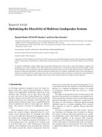
in different order. A biological example of the latter is
given in the simple case of linear sets of transformations
in Figure 1, where rectangles are reactions and circles
are compounds. More complex examples are discussed in
Lacroix et al. [12].
Moreover, in some situations, as, for example, in the case
of protein interaction networks, the topology of the network
is not fully known. Indeed, high-throughput experiments
used to obtain large-scale protein interaction data are notori-
ously noisy, that is, they may detect interactions when there is
none (false positive) and they may miss existing interactions
(false negative). In this context, it may be inadequate to look
for exact repetitions of a pattern. An alternative definition
has thus been proposed, where a motif is defined by using the
labels of its vertices and only connectedness of the induced
subgraph is required [12].
A coloured motif is defined as a multiset of colours
(vertex labels), that is, a motif may contain colours whose
multiplicity are greater than 1. The cardinality of a motif,
that is, of the multiset, will be called the size of a motif. An

occurrence of a motif is defined as a connected subgraph
whose labels match the motif.
The enumeration of coloured motifs is a nontrivial task
which has been the subject of several works [12, 13]which
allowed to establish the complexity of the problem and
provide algorithms to efficiently detect all the occurrences of
a motif in a graph. In practice, current methods now allow
to enumerate all the motifs of size 7 of a graph representing
the metabolic network of a bacterium in less than two hours.
Beyond the time complexity of the task, a major challenge
that remains open is to make sense of the potentially very
large output of such an enumeration procedure, especially
whenthefocusisnotonasinglemotifbutonallmotifs
of a given size. Ideally, one would need a method to rank
the motifs according to their biological relevance in order to
prioritise a small number of motifs for downstream analysis.
However, the notion of biological relevance is generally ill
defined, and a classically used approximation is its statistical
significance (or exceptionality).
The exceptionality of a coloured motif, that is the
over- or under-representation of the motif with respect
to a null model, can be assessed by comparing the
observed count of occurrences of a motif to the expected
count of the same motif under a null hypothesis. Up
to now, this procedure was performed (e.g., in MOTUS
[14], using simu-
lations: a large number of random graphs were generated
and the motif of interest was sought in each one, generating
an empirical distribution of the motif count to which the
observed count could be compared in order to derive a z-

score and a P-value. The main limitation of this procedure
is that it adds a multiplicative factor to the time complexity
of the algorithm. Moreover, it is not trivial to choose the
optimal number of simulations to perform in order to get
a satisfactory estimation of the P-value. As a rule of thumb,
in order to estimate quite accurately a P-value of 1 over 10
i
,
at least 10
i+2
simulations should be performed.
In this paper, we propose a new approach for assessing
the exceptionality of coloured motifs which do not require
simulations and therefore circumvents the previously men-
tioned limitations. We were able to establish exact analytical
formulae for the mean and the variance of the count of
a coloured motif in an Erd
¨
os-R
´
enyi (ER) random graph
model. Thanks to these results, one can now derive a z-score
for each motif and therefore rank them according to their
exceptionality. We then worked on modelling the complete
distribution of the count of a coloured motif in an ER
randomgraphmodel.Tothispurpose,weperformedalarge
number of simulations, using different colour frequencies
for the motif and different number of vertices and edges for
the graph. We could establish that the Poisson distribution
was not appropriate whereas the P

´
olya-Aeppli distribution
was a good and better approximation than the commonly
used Gaussian distribution. The choice of a P
´
olya-Aeppli
distribution was driven by the following facts: (i) motif
occurrences overlap in a network, as shown in Figure 1; (ii)
compound Poisson distributions are particularly adapted to
model counts of clumping events [15, Chapter 9]; (iii) P
´
olya-
Aeppli approximations are efficient for the count of words in
letter sequences [16]. These results can in turn be used to
derive a P-value for each motif, and, therefore, to introduce
a cut-off for deciding which motifs should be selected for
downstream analysis.
To our knowledge, there has been no previous work on
the significance of coloured motifs in random graphs. This is
EURASIP Journal on Bioinformatics and Systems Biology 3
Acetolactate
2,3-dihydroxy-isovalerate
1.1.1.86
1.1.1.85
1.1.1.37
1.1.1.38
1.1.1.40
1.1.1.86
4.2.1.9
4.2.1.9

4.2.1.2
4.2.1.33
2.6.1.42
2.6.1.42
2.6.1.42
2.6.1.1
2.6.1.42
2-keto-isovalerate
L-valine
L-isoleucine
2-isopropylmalate
3-isopropylmalate
2-ketoisocaproate
L-leucine
2-aceto-2-hydroxy-butyrate
2,3-dihyroxy-3-methylvalerate
2-keto-3-methyl-valerate
Fumarate
Malate
Oxaloacetate
L-aspartate
L-alanine
Pyruvate
2.6.1.2
Figure 1: Similar sets of transformations in the metabolic network of the bacterium Escherichia c oli.
the reason why we started by focusing on the more general
random graph model that is available. We are aware that this
may not be the most suitable model to describe the structure
of a biological network. However, we argue that this work
provides a first necessary basis which can later be extended to

richer models, such as the promising mixture of Erd
¨
os-R
´
enyi
models proposed by Daudin et al. [17].
2. Definitions and Notations
Coloured Random Graph Model. We consider a random
graph G with n vertices
{V
1
, , V
n
}. We assume that
random edges are independent and distributed according to
a Bernoulli distribution with parameter p
∈]0, 1] (the so-
called Erd
¨
os-R
´
enyi model). Moreover, vertices are randomly
and independently coloured as follows. Let C be a finite set
of r different colours and f a probability measure on C: f (c)
is then the probability for a vertex to be coloured with c
∈ C.
In a metabolic network, the colours of reaction
vertices can represent classes of chemical transforma-
tions; in regulation networks, the colours of gene ver-
tices can represent functional classes. For defining these

classes, the EC number hierarchy (
.uk/iubmb/enzyme/)orGeneOntology(e-
ontology.org/GO.doc.shtml) is classically used.
Coloured Motif. We consider motifs as introduced in Lacroix
et al. [12]:a(coloured)motifm of size k is a multiset of k
colours
{m
1
, , m
k
}∈C
k
. Colours from a motif may not be
different, that is, one may have m
i
= m
j
for some 1 ≤ i, j ≤ k.
We then denote by s
m
(c) the multiplicity of the colour c in m.
When there is no ambiguity, s
m
(c) will simply be denoted by
1
32
45
9
10
6

7
8
m ={ }
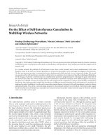
Figure 2: Example of a graph and a motif. The motif m occurs
three times in the graph, at positions
{2, 4, 5, 9}, {1, 3, 7, 8},and
{3, 6, 7, 8}.
s(c). The notion of multiplicity of a single colour in m will be
extended to a multiset of colours in Section 3.2.
Motif Occurrences. We now define an occurrence of such a
coloured motif. To this purpose, we introduce the following
notation. If i
1
, i
2
, , i
k
are k different indices from {1, , n},
then G(i
1
, i
2
, , i
k
) represents the subgraph of G induced by
the vertices
{V
i
1
, , V

i
k
}.LetI
k
be the set of all the subsets of
size k from
{1, , n}. We say that a motif m ={m
1
, , m
k
}
occurs at position α ={i
1
, , i
k
}∈I
k
if and only if G(α)
is connected and the colours of G(α), denoted by C(α),
are exactly
{m
1
, , m
k
}. I
k
corresponds, then, to the set of
possible positions for the occurrence of a motif of size k.
Figure 2 gives an example of a motif and its occurrences.
Number of Occurrences. We introduce the random indicator

variable Y
α
(m) which equals one if motif m occurs at
4 EURASIP Journal on Bioinformatics and Systems Biology
position α
∈ I
k
in G and zero, otherwise
Y
α
(m) = I{m occurs at position α},(1)
where Y
α
(m) is then a Bernoulli random variable whose
expectation is denoted by μ(m):
μ(m)
= EY
α
(m) = P(m occurs at position α). (2)
The probability μ(m)form to occur at position α will be
given in Section 3.1.
The number of occurrences of the motif m in the graph
G,denotedbyN(m), is defined by
N(m)
=

α∈I
k
Y
α

(m). (3)
3. Mean and Variance for the Count
This section will provide analytical formulae for the mean
and the variance of the number of occurrences of a coloured
motif in a random graph. It involves the computation of
some probabilities of connectedness. The generalisation to
the number of occurrences of a set a coloured motifs will be
done in the supplementary material.
3.1. Mean Number of Occurrences. The mean number of
occurrences of the motif m in the graph G simply follows
from the count expression (3):
EN(m) =

α∈I
k
EY
α
(m) =

n
k

μ(m), (4)
where μ(m) is the occurrence probability of the motif and is
given below by (6).
Occurrence Probability. The probability μ(m)form to occur
at position α
= (i
1
, , i

k
) is simply equal to the product
of two probabilities: the probability that G(α) is connected
and the probability to assign colours
{m
1
, , m
k
} to vertices
{V
i
1
, , V
i
k
}. The latter, denoted by γ(m), follows from the
multinomial distribution
γ(m)
=
k!

c∈C
s(c)!
k

i=1
f

m
i


,(5)
leading to
μ(m)
= g(k, p) × γ(m), (6)
where g(k, p) denotes the probability for a random graph
(Erd
¨
os-R
´
enyi model) with k vertices and edge probability p
to be connected (by definition, 0!
= 1).
Connectivity Probability. The probability g(k, p) is calculated
recursively [18] as follows:
g(k, p)
= 1 −
k−1

i=1

k −1
i
−1

g(i, p)(1 − p)
i(k−i)
,(7)
where g(1, p)
= 1. For instance, for 2 ≤ k ≤ 5, which is

typically the range for the motif size in practice, we have
g(2, p)
= p,
g(3, p)
= 3p
2
−2p
3
,
g(4, p)
= 16p
3
−33p
4
+24p
5
−6p
6
,
g(5, p)
= 125p
4
−528p
5
+ 970p
6
−980p
7
+ 570p
8

−180p
9
+24p
10
.
(8)
3.2. Variance of the Number of Occurrences. Getting the
variance is much more involved. We start from Var N(m)
=
E
N
2
(m) − (EN(m))
2
and we have to compute the moment
of order two
EN
2
(m) =

α∈I
k

β∈I
k
E

Y
α
(m)Y

β
(m)

. (9)
First, the sums over α and β are calculated according to the
number  of vertices shared by the subgraphs G(α)andG(β):
EN
2
(m) =
k

=0

|α∩β|=
E

Y
α
(m)Y
β
(m)

. (10)
Second, we use the fact that Y
α
(m)andY
β
(m) are indicator
variables which lead to
E[Y

α
(m)Y
β
(m)] = P(Y
α
(m) =
1andY
β
(m) = 1). These random variables are not indepen-
dent but the above probability can be written as
E

Y
α
(m)Y
β
(m)

=
K(α, β) ×Q
m
(α, β), (11)
with
K(α, β)
= P(G(α)andG(β) are connected),
Q
m
(α, β) = P

C(α) = C(β) =


m
1
, , m
k

.
(12)
The terms K(α, β)andQ
m
(α, β) are now separately calcu-
lated.
Computation of Q
m
(α, β). Let  =|α ∩ β|; the subgraphs
G(α)andG(β)havethus vertices in common, with 0
≤
 ≤ k.Letm
∗
⊂ m such that |m
∗
|= and denote
m
−
= m \ m
∗
; m
∗
represents the colours of the  vertices
shared by G(α)andG(β). The multiplicity of colour c

∈ C
in m
∗
(resp., in m
−
)isdenotedbys
∗
(c)(resp.,s
−
(c)). To
calculate
P(C(α) = C(β) = m), we start by choosing the 
colours m
∗
of G(α) ∩ G(β)(eventwithprobabilityγ(m
∗
)),
then the (k
− ) remaining colours m
−
are spread over both
G(α)
\ (G(α) ∩ G(β)) (event with probability γ(m
−
)) and
G(β)
\(G(α)∩G(β)) (event with probability γ(m
−
)). Finally,
one just has to sum over all possible different m

∗
⊂ m which
is equivalent to summing over all m
∗
⊂ m and dividing each
term by the multiplicity of m
∗
in m.Thisleadsto
Q
m
(α, β) =

m
∗
⊂m
γ

m
∗

γ

m
−

2
s

m
∗


, (13)
where s(m
∗
) = s
m
(m
∗
) is the multiplicity of m
∗
in m.For
instance, if C
={1,2, 3}, m ={1, 3, 1, 2},and = 2, then
the multiplicity of m
∗
={1, 3} in m equals 2 whereas the
multiplicity of m
∗
={1,1} equals 1.
EURASIP Journal on Bioinformatics and Systems Biology 5
Computation of K(α, β). Let again 
=|α ∩ β|.If =
0(i.e.,G(α)andG(β) are disjoint) or  = 1(i.e.,
G(α)andG(β) have a unique vertex in common) then
the events
{G(α) is connected} and {G(β) is connected} are
independent leading to
K(α, β)
= g
2

(k, p), if  = 0or1. (14)
Another easy case is when 
= k because it means that β = α
and therefore
K(α, β)
= g(k, p), if  = k. (15)
For the other cases, no general formulae have been found so
far but for small values of k one can automatically enumerate
all the solutions thanks to the edge binary tree, as described
below. As an illustration, the case k
= 3(and = 2) will be
detailed.
The principle is to work conditionally to the subgraph
G(α)
∩G(β)
P(G(α)andG(β) are connected)
=

G

P(G(α) ∩ G(β) = G

)
×

P(G(α) connected | G(α) ∩ G(β) = G

)

2

,
(16)
where G

is any subgraph of  vertices. Since k is typically
small, both probabilities can be computed by enumerating
all possible subgraphs G

and G(α). This can be done by
traversing the complete edge binary tree associated to the
k(k
− 1)/2potentialedgesofG(α), that is, to the binary
tree whose branches are labelled according to the presence
or absence of edges in the subgraph G(α). This tree is
composed of k(k
− 1)/2 levels, one for each potential edge
and each internal vertex in this tree has two sons: the
left one corresponds to the presence of the corresponding
edge in the graph whereas the right one corresponds to its
absence. It follows that each path from the root to a leaf
corresponds to one of the 2
k(k−1)/2
possible graphs of size k.
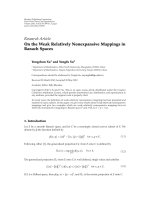
Figure 3 gives an example for k
= 3. Vertices are labelled
{i, j, u}, the higher level corresponds to the edge (i, j), the
middle one corresponds to the edge (i, u), and the lower
level corresponds to the edge (j, u). Leaves corresponding
to connected graphs are drawn with a square. In practice,
the connectedness of a graph can be checked thanks to its

adjacency matrix to the power k
− 1. Indeed, a graph of size
k with adjacency matrix A is connected if and only if A
k−1
contains no zero (every vertex can be reached from any vertex
in at most k
− 1 steps). Additionally, the binary tree is built
such that all pairs of common vertices between G(α)and
G(β) are at the top levels. The probability of each connected
graph of size k can then be easily calculated when traversing
the tree and likewise for both probabilities appearing in (16).
As an illustration, we now detail the computation for
k
= 3and = 2. Let i and j be the two common vertices
between G(α)andG(β), and let u be the third vertex of G(α)
(α
={i, j, u}). The edge binary tree is given by Figure 3.In
this case, there are only two subgraphs G

with  = 2vertices:
either i and j are connected (probability p) or they are not
connected (probability 1
− p). In Figure 3, we indicate with
a dashed horizontal line the separation between edges in G

(the conditioning event) and edges in G(α)\G

.Overall,with
k
= 3, there are four possible connected subgraphs G(α): the

triangle (labelled by “a”) and the three possible “Vs” (labelled
by “b”, “c”, and “d”). The probability that G(α) is connected
given i
↔j is obtained from cases “a” (probability p
2
), “b”
(probability p(1
− p)), and “c” (probability p(1 − p))
P(G(α) connected | i ←→ j) = p
2
+2p(1 − p) = 2p − p
2
.
(17)
The probability that G(α) is connected given that i is not
connected with j is obtained from case “d” (probability p
2
),
leading to
P(G(α)andG(β) are connected)
= p ×

2p − p
2

2
+(1− p) ×

p
2


2
= 4p
3
−3p
4
.
(18)
Using this algorithm, we find the following results for k
=
3andk = 4(k = 2 can be processed with the trivial formulae
(14)or(15)):
k
= 3,  = 2: K(α, β) = 4p
3
−3p
4
,
k
= 4,  = 2: K(α, β) = 64p
5
−160p
6
+ 100p
7
+77p
8
−136p
9
+68p

10
−12p
11
,
k
= 4,  = 3: K(α, β) = 27p
4
−60p
5
+46p
6
−12p
7
.
(19)
Finally, we obtained analytical formulae for the variance.
4. Towards the Motif Count Distribution:
A Simulated Approach
Aim. No theoretical results exist so far on the distribution
of coloured motifs in random graphs. In this paper, we
propose an approximation for this distribution. Thanks
to simulations, we first studied the quality of the normal
approximation which is classically assumed, especially when
using z-scores [5, 12]. However, network motif occurrences
tend to overlap in networks. It is well known from prob-
ability theory that compound Poisson distributions are
more relevant than Gaussian distributions to model the
count of rare and clumping events. Besides, a compound
Poisson approximation for the count of particular subgraphs
(topological network motifs) has been proposed by Stark

[8] under certain asymptotic conditions on the ER random
graph model. Moreover, by analogy with pattern occur-
rences in letter sequences [16], Picard et al. [11] recently
investigated a particular compound Poisson approximation,
namely, a P
´
olya-Aeppli approximation, and concluded that
this distribution fits well the count of topological network
motifs. The P
´
olya-Aeppli distribution (denoted by PA)with
parameters (λ, a) is the distribution of

C
c=1
K
c
, where the
number of clumps C is Poisson distributed (C
∼P (λ)) and
the size K
c
of the clumps is geometrically distributed (P(K
c
=
6 EURASIP Journal on Bioinformatics and Systems Biology
a
b
c
d

ij
ij
iu
iu iu iu
ju
ju ju ju ju ju ju ju
∅∅∅∅
Figure 3: Complete edge binary tree for vertices i, j,andu. Branches are labelled according to the presence or absence of edges: label ij,for
instance, means that i and j are connected, whereas
ij means the opposite. Leafs which correspond to connected subgraphs are represented
by a square.
k) = (1 − a)a
k
). Its mean is equal to λ/(1 − a) and its
variance equals λ(1+a)/(1
−a)
2
. We have then also considered
the P
´
olya-Aeppli approximation. We did not investigate the
Poisson approximation because, as we can see on Tabl e 1, the
variance of the count (whatever the coloured motif) is quite
different from the mean count.
Simulation Design. We have simulated 10 000 Erd
¨
os-R
´
enyi
random graphs with n vertices (n

∈{100, 500, 1000})and
edge probability P
∈{.05, .01, .005}.Verticeshavebeen
randomly coloured with 5 colours (C
={1, 2, 3, 4, 5})
and according to the following colour frequencies: f
=
(50, 25, 10, 5, 1)/91. These choices for n, p,and f allow to
get coloured motifs of size 3 with a wide range of expected
counts. We have then selected 14 motifs of size 3 to cover
both this variety of counts and different multiplicity pat-
tern:
{1, 1, 1}, {1, 2, 2}, {1, 2, 3}, {1, 1, 4}, {1, 3, 4}, {1,1, 5},
{2, 4, 4}, {4, 4, 4}, {2, 4, 5}, {3, 4, 5}, {1, 5, 5}, {3, 5, 5},
{4, 5, 5},and{5,5, 5}.
For each motif and each couple (n, p), we then obtained
an empirical distribution which has been compared with
both the normal distribution N (

E
N(m),

VarN(m)) and the
P
´
olya-Aeppli distribution PA(

λ, a)with

λ = (1 −a)


E
N(m)
and
a = [

VarN(m) −

EN(m)]/[

VarN(m)+

E
N(m)] (see
Figure 4 for 4 representative examples).
Quality of Approximation. To measure this quality, we
adopted two criteria: (1) the Kolmogorov-Smirnov distance
which measures the maximal difference between the empir-
ical cumulative distribution function (cdf)

F and the cdf of
the normal or the P
´
olya-Aeppli distribution. The closer to 0
the KS distance, the better the approximation. (2) 1 minus
the empirical cdf calculated at the 99% and 99.9% quantiles
of the normal or of the P
´
olya-Aeppli distribution. The closer
to 1% and 0.1% these values, the better the approximation.

Results. Results for different values of n and p are very
similar. We only present here the ones corresponding to
n
= 500 and P = .01 because these values are very close to
those observed in real cases such as the metabolic network of
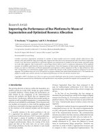
E. coli as considered in Lacroix et al. [12]. Nevertheless, all
results are presented in the supplementary material.
We can first notice just by eye (see Figure 4) that the
normal distribution seems satisfactory for frequent motifs
but the rarer the motif, the worse the goodness-of-fit. The
P
´
olya-Aeppli distribution seems to fit quite correctly the
count distribution whatever the motif. These initial impres-
sions are emphasised when we look at the Kolmogorov-
Smirnov distances (see Ta bl e 1). The ones for the P
´
olya-
Aeppli distribution are always smaller than those for the
normal distribution and sometimes much smaller. In fact,
the distance to the normal distribution is quite large for
very rare motifs (typically when
EN(m) ≤ 10). If we
now concentrate on the distribution tails by looking at
the empirical probabilities to exceed the 99% or 99.9%
quantiles q
N
and q
PA
, we can also notice that they are

closer to 1% or 0.1% for the P
´
olya-Aeppli distribution
than for the normal distribution. For extremely rare motifs,
quantiles q
PA
for both 99% and 99.9% could not be
correctly calculated because the corresponding P
´
olya-Aeppli
distribution is both discrete and concentrated around 0.
The values for the empirical tails provided in the table are
therefore not meaningful in such cases, but thanks to the very
small KS distances, we can check that the approximation is
still good. Finally, observe that most of the time the normal
distribution underestimates the quantile (the empirical right
tail is overestimated) leading to false positives.
5. Discussion and Conclusion
In this paper, we proposed a new way to assess the
exceptionality of coloured motifs in networks which do not
require to perform simulations. Indeed, we were able to
establish analytical formulae for the mean and the variance
EURASIP Journal on Bioinformatics and Systems Biology 7
0
0.001
0.002
0.003
0.004
Density
300 400 500 600 700 800 900 1000

Counts
Motif 123 (n
= 500, P = .01)
empirical mean = 615.2566
(a)
0
0.002
0.004
0.006
0.008
0.01
0.012
Density
0 50 100 150 200 250
Counts
Motif 115 (n
= 500, P = .01)
empirical mean = 61.7187
(b)
0
0.01
0.02
0.03
0.04
0.05
Density
0 10203040506070
Counts
Motif 244 (n
= 500, P = .01)

empirical mean = 15.2864
(c)
0
0.05
0.1
0.15
0.2
0.25
Density
0 5 10 15 20
Counts
Motif 345 (n
= 500, P = .01)
empirical mean = 2.5112
(d)
Figure 4: Empirical distributions for the count of motifs {1,2,3}, {1, 1, 5}, {2, 4, 4},and{3, 4, 5} in random graphs with n = 500 and
P
= .01. The empirical means are, respectively, 615, 61, 15, and 2. The red (resp., green) curves correspond to the ad hoc normal distributions
(resp., P
´
olya-Aeppli distributions).
of the count of a coloured motif in an Erd
¨
os-R
´
enyi random
graph model. Furthermore, using simulations, we showed
that the motif count distribution can be quite accurately
approximated with a P
´

olya-Aeppli distribution, and that
neither the Gaussian nor the Poisson distributions are
relevant. Altogether, these results now allow to derive a P-
value for a coloured motif without performing simulations.
Clearly, when several motifs have to be tested, which is the
case in the context of motif discovery, one has to control
for multiple testing. A conservative strategy that is classically
used and that we would recommend is then to apply a
Bonferroni correction.
In this work, we did not investigate the case of long
motifs, but we can anticipate that motifs containing sub-
motifs which are exceptional will tend to be exceptional
themselves. This type of phenomenon is also observed for
patterns in sequences and a classical way to deal with it is to
control for the number of sequence patterns of size k
−1(by
using a Markov model of order k
− 2), when assessing the
exceptionality of patterns of size k. However, in the case of
networks, the problem is far from trivial and it is unclear,
even for small values of k if the space of random graphs
verifying these constraints will not be too small. In the worst
case, this space may even be reduced to the observed graph
itself.
Also in the case of very rare motifs, the expected
distribution of the count is essentially concentrated around
0. Therefore, a single occurrence of such a motif will often
be sufficient for it to be considered as exceptional. If we now
consider the extreme case of a coloured graph, where each
vertex is assigned a different colour, then all possible motifs

will be very rare and, therefore, they may all be detected
as exceptional. In practical cases, such as for the network
representing the metabolic network of the bacterium E. coli,
the situation is less dramatic but indeed many colours are
present only once. This issue may be partially addressed
by considering a random graph model, where the colours
and the topology are not independent anymore. This would
allow to discriminate between infrequent poorly connected
colours and infrequent highly connected colours. Motifs
8 EURASIP Journal on Bioinformatics and Systems Biology
Table 1: Quality of approximation of the count distribution for n = 500 and P = .01. The empirical mean

E
N(m), variance

VarN(m),
and cumulative distribution function

F have been obtained thanks to 10 000 random graphs. (a,

λ) are the parameters of the P
´
olya-Aeppli
distribution. KS
N
and KS
PA
are the Kolmogorov-Smirnov distances. For α = 1% then 0.1%, q
N
is the 1 − α quantile of the normal

distribution (idem for the P
´
olya-Aeppli distribution).
α = 1% α = 0.1%
Motif
m
EN(m)VarN(m)

E
N(m)

VarN(m) a

λ
KS
N
(%)
KS
PA
(%)
q
N
1 −

F(q
N
)
(%)
q
PA

1 −

F(q
PA
)
(%)
q
N
1 −

F(q
N
)
(%)
q
PA
1 −

F(q
PA
)
(%)
111
1023.65 27462.66 1021.97 27446.53 0.93 73.37
2.40 0.78
1407.4
1.6
1436
1.1
1533.9

0.23
1591
0.12
122
767.74 14941.43 766.05 14660.79 0.90 76.08
2.14 0.65
1047.7
1.5
1068
1.0
1140.2
0.25
1181
0.07
123
614.19 8546.68 615.26 8493.22 0.86 83.12
1.75 0.68
829.6
1.4
845
0.8
900.0
0.18
929
0.08
114
307.09 5729.89 307.77 5807.09 0.90 30.98
3.20 0.71
485.0
1.5

505
0.8
543.3
0.28
583
0.08
134
122.84 1305.02 123.06 1311.64 0.83 21.11
3.43 0.78
207.3
1.8
219
0.9
235.0
0.37
257
0.12
115
61.41 1180.68 61.72 1147.95 0.90 6.30
5.72 0.98
140.5
2.3
160
0.8
166.4
0.57
205
0.06
244
15.35 85.99 15.29 85.57 0.70 4.63

8.73 1.07
36.8
2.4
43
0.8
43.9
0.81
55
0.12
245
6.14 27.76 6.20 28.45 0.64 2.22
12.72 1.27
18.6
2.5
23
0.8
22.7
1.09
32
0.10
345
2.46 6.63 2.51 6.58 0.45 1.39
17.97 0.53
8.5
1.9
11
0.5
10.4
0.77
15

0.09
155
1.23 6.94 1.22 6.74 0.69 0.37
34.23 5.75
7.2
3.3
12
0.6
9.2
1.56
20
0.05
444
1.02 2.46 1.02 2.51 0.42 0.59
27.39 3.80
4.7
2.4
7
0.5
5.9
1.48
10
0.09
355
0.25 0.50 0.25 0.50 0.34 0.16
48.47 0.43
1.9
2.5
3
0.4

2.4
0.96
6
2e-05
455
0.12 0.20 0.13 0.20 0.23 0.09
51.63 0.16
1.2
0.6
2
0.1
1.5
0.65
4
0.03
555
0.008 0.01 0.007 0.008 0.035 0.007
52.61 2e-03
0.2
0.03
0
0.03
0.3
0.03
1
2e-05
containing the latter type of colours would be expected
to have more occurrences and should therefore not be
systematically considered as exceptional when they have a
single occurrence.

More generally, we considered in this paper a very
simple random graph model. Even though we think this
work was necessary to establish a framework for accessing
the exceptionality of coloured motifs, an important step is
now to extend these results to other models of random
graphs which better represent the structure of real networks.
Different types of models have been proposed in the liter-
ature for this purpose, for instance, small-world networks,
scale-free networks, preferential attachment models, and
fixed degree distribution models. However, these models do
not provide the probabilistic distribution on edges which
is required to compute the occurrence probability of a
motif and the probability of two nondisjoint occurrences.
Moreover, it has been shown that subnetworks of scale-free
networks lose the scale-free property [19]. This is a real
drawback for modelling biological networks because they
usually correspond to the partial knowledge we have of a
system and are therefore far from complete. An interesting
issue would be to generalise our work to a mixture of
ER random graph models. These models seem indeed
very flexible and are able to fit nicely biological networks
[17].
Finally, we think there is still room for improvement
on the approximation of the motif count distribution.
Indeed, no theoretical evidence has been found so far
supporting the use of a geometric distribution for the clump
size. Analytically, getting the third moment and eventually
the fourth moment of the count could certainly allow to
investigate other distributions.
Acknowledgments

The authors would like to thank Etienne Birmel
´
e, Jean-
Jacques Daudin, Catherine Matias, and St
´
ephane Robin
for helpful discussions about the moment calculations.
They particularly thank Jean-Jacques Daudin for providing
a MATLAB program to automatically compute the term
K(α, β). They also thank the anonymous reviewers for
their helpful comments and suggestions for improving
the manuscript. This work has been supported by the
ANR (NEMO Project BLAN08-1
318829, REGLIS Project
NT05-3
45205, and MIRI Project BLAN08-1 335497) and
the ANR-BBSRC (MetNet4SysBio Project ANR-07-BSYS
003 02).
References
[1] E. Alm and A. P. Arkin, “Biological networks,” Current
Opinion in Structural Biology, vol. 13, no. 2, pp. 193–202, 2003.
[2]H.Jeong,B.Tombor,R.Albert,Z.N.Oltvai,andA L.
Barab
´
asi, “The large-scale organization of metabolic net-
works,” Nature, vol. 407, no. 6804, pp. 651–654, 2000.
[3] S. Maslov and K. Sneppen, “Specificity and stability in
topology of protein networks,” Science, vol. 296, no. 5569, pp.
910–913, 2002.
[4] A. Wagner and D. A. Fell, “The small world inside large

metabolic networks,” Proceedings of the Royal Society B, vol.
268, no. 1478, pp. 1803–1810, 2001.
EURASIP Journal on Bioinformatics and Systems Biology 9
[5] R.Milo,S.S.Shen-Orr,S.Itzkovitz,N.Kashtan,D.Chklovskii,
and U. Alon, “Network motifs: simple building blocks of
complex networks,” Scie nce , vol. 298, no. 5594, pp. 824–827,
2002.
[6] S. S. Shen-Orr, R. Milo, S. Mangan, and U. Alon, “Network
motifs in the transcriptional regulation network of Escherichia
coli,” Nature Genetics, vol. 31, no. 1, pp. 64–68, 2002.
[7] S. Janson, T. Łuczak, and A. Ruci
´
nski, Random Graphs, Wiley-
Interscience, New York, NY, USA, 2000.
[8] D. Stark, “Compound Poisson approximations of subgraph
countsinrandomgraphs,”Random Structures & Algorithms,
vol. 18, no. 1, pp. 39–60, 2001.
[9] S. Itzkovitz, R. Milo, N. Kashtan, G. Ziv, and U. Alon,
“Subgraphs in random networks,” Physical Review E, vol. 68,
no. 2, Article ID 026127, 8 pages, 2003.
[10] J. Camacho, D. B. Stouffer, and L. A. N. Amaral, “Quantitative
analysis of the local structure of food webs,” Journal of
Theoretical Biology, vol. 246, no. 2, pp. 260–268, 2007.
[11] F. Picard, J J. Daudin, M. Koskas, S. Schbath, and S. Robin,
“Assessing the exceptionality of network motifs,” Journal of
Computational Biology, vol. 15, no. 1, pp. 1–20, 2008.
[12] V. Lacroix, C. G. Fernandes, and M F. Sagot, “Motif search
in graphs: application to metabolic networks,” IEEE/ACM
Transactions on Computational Biology and Bioinformatics, vol.
3, no. 4, pp. 360–368, 2006.

[13] M. R. Fellows, G. Fertin, D. Hermelin, and S. Vialette, “Sharp
tractability borderlines for finding connected motifs in vertex-
colored graphs,” in Proceedings of the 34th International Collo-
quium on Automata, Languages and Programming (ICALP ’07),
vol. 4596 of Lecture Notes in Computer Science, pp. 340–351,
Wroclaw, Poland, July 2007.
[14] V. Lacroix, L. Cottret, O. Rogier, C. Fernandes, F. Jourdan, and
M F. Sagot, “Motus: a software and a webserver for thesearch
and enumeration of node-labelled connected subgraphs in
biological networks,” submitted.
[15]N.L.Johnson,S.Kotz,andA.W.Kemp,Univariate Discrete
Distributions, John Wiley & Sons, New York, NY, USA, 1992.
[16] S. Schbath, “Compound Poisson approximation of word
counts in DNA sequences,” ESAIM: Probability and Statistics,
vol. 1, pp. 1–16, 1995.
[17] J J. Daudin, F. Picard, and S. Robin, “A mixture model for
random graphs,” Statistics and Computing,vol.18,no.2,pp.
173–183, 2008.
[18] E. N. Gilbert, “Random graphs,” The Annals of Mathematical
Statistics, vol. 30, no. 4, pp. 1141–1144, 1959.
[19] M. P. H. Stumpf, C. Wiuf, and R. M. May, “Subnets of
scale-free networks are not scale-free: sampling properties of
networks,” Proceedings of the National Academy of Sciences of
the United States of America, vol. 102, no. 12, pp. 4221–4224,
2005.