Báo cáo hóa học: " Research Article Automatic Music Boundary Detection Using Short Segmental Acoustic Similarity in a Music Piece" potx

Hindawi Publishing Corporation
EURASIP Journal on Audio, Speech, and Music Processing
Volume 2008, Article ID 480786, 10 pages
doi:10.1155/2008/480786
Research Article
Automatic Music Boundary Detection Using Short Segmental
Acoustic Similarity in a Music Piece
Yoshiaki Itoh,
1
Akira Iwabuchi,
1
Kazunori Kojima,
1
Masaaki Ishigame,
1
Kazuyo Tanaka,
2
and Shi-Wook Lee
3
1
Faculty of Software and Information Sci ence, Iwate Prefectural University, Sugo, Takizawa, Iwate 020-0193, Japan
2
Institute of Library and Information Science, University of Tsukuba 1-2 Kasuga, Tsukuba 305-8550, Japan
3
National Institute of Advanced Industrial Science and Technology (AIST), Agency of Industrial Science and Technology,
Tukuba-shi Ibaragi, 305-8568, Japan
Correspondence should be addressed to Yoshiaki Itoh,
Received 2 November 2007; Revised 15 February 2008; Accepted 27 May 2008
Recommended by Woon-Seng Gan
The present paper proposes a new approach for detecting music boundaries, such as the boundary between music pieces or
the boundary between a music piece and a speech section for automatic segmentation of musical video data and retrieval of a

designated music piece. The proposed approach is able to capture each music piece using acoustic similarity defined for short-
term segments in the music piece. The short segmental acoustic similarity is obtained by means of a new algorithm called
segmental continuous dynamic programming, or segmental CDP. The location of each music piece and its music boundaries
are then identified by referring to multiple similar segments and their location information, avoiding oversegmentation within
a music piece. The performance of the proposed method is evaluated for music boundary detection using actual music datasets.
The present paper demonstrates that the proposed method enables accurate detection of music boundaries for both the evaluation
data and a real broadcasted music program.
Copyright © 2008 Yoshiaki Itoh et al. This is an open access article distributed under the Creative Commons Attribution License,
which permits unrestricted use, distribution, and reproduction in any medium, provided the original work is properly cited.
1. INTRODUCTION
Hard discs have recently come into widespread use, and
the medium of the home video recorder is changing from
sequential videotape to media such as random accessible
hard discs or DVDs. Such media can store recording
video data of great length (long-play video data) and play
stored data at any location in the media immediately. In
conjunction with the increasingly common use of such long-
play video data, the demand for retrieval and summarization
of data has been growing. In addition, detailed descriptions
of the content associated with correct time information are
not usually attached to the data, although topic titles can be
obtained from electronic TV programs and attached to the
data. Automatic extraction of each music piece is meaningful
for the following reasons. Some users who enjoy watching
music programs want to listen to the start of each music
piece, omitting the conversations between music pieces, and
other users want to view the speech conversational sections.
Therefore, automatic detection of music boundaries between
music pieces, or between a music piece and a speech section,
is necessary for indexing or summarizing video data. In the

present paper, a music piece refers to a song or a musical
performance by an artist or a group, such as “Thriller” by
Michael Jackson.
The present paper proposes a new method for identifying
the location of each music piece and detecting the boundaries
between music pieces avoiding oversegmentations within
a music piece for automatic segmentation of video data.
The proposed method employs an acoustic similarity of
short-term segments in a music and speech stream. The
similarity is obtained by means of segmental continuous
dynamic programming, called segmental CDP. In segmental
CDP, a set of video acoustic streaming data is divided
into segments of fixed length, for example, 2 seconds.
Continuous DP is performed on the subsequent acoustic
data, and similar segments are obtained for each segment [1].
When segment A matches a subsequent segment, namely,
2 EURASIP Journal on Audio, Speech, and Music Processing
segment B, segments A and B are similar and are considered
to fall within the same music piece. However, different
music pieces are expected to have few similar segments.
Therefore, the location and the boundaries of a music piece is
identified using the location and the frequency information
between similar segments of fixed length. This approach is an
extension of topic identification, as described in [2].
Some studies reported music retrieval applications in
which the target music is identified by a query music section
[3, 4].Anumberofstudies[4–9] have proposed methods
for acoustic segmentation that is primarily based upon the
similarity and dissimilarity of local feature vectors. The
performance in these studies was evaluated based on the

correct discrimination ratio of frames [7–9] and not on
the correct discrimination ratio of music boundaries. Using
these methods, music boundaries are difficult to detect when
music pieces are played continuously as they are in usual
music programs. Our preliminary experiments showed that
the GMM, which is a typical method of discrimination
between music and voice, could not detect music boundaries
in continuous music pieces. Dynamic programming has
already been used to follow the sequence of similar feature
vectors and to detect boundaries between music and speech
and between music pieces [10]. This type of methods is likely
to detect unnecessary boundaries such as points of modula-
tion and changes in musical instruments as described [10].
Vocal sections without instruments were also determined
as boundaries in our preliminary experiments, and related
studies have not been able to avoid oversegmentation within
a music piece. The proposed method can capture the location
of a music piece using acoustic similarity within the piece and
avoid oversegmentation.
First, the present paper describes an approach for
detecting music boundaries, with the goal of automatic
segmentation of video data such as musical programs.
The concept and the segmental CDP algorithm are then
explained, along with the methodologies for identifying the
music boundaries using similar segments that are extracted
by segmental CDP. The feasibility of the proposed method is
verified by experiments on music boundary detection using
open music datasets supplied by the RWC project [11], and
by applying the method to an actual broadcasted music
program.

2. PROPOSED APPROACH
2.1. Outline of the proposed system
Generally speaking, in music, especially in popular music,
the same melody tends to be repeated, such that the first
and second verses have the same melody but different words
and the main melody is repeated several times. Each music
piece is assumed to have acoustically similar sections within
the music piece. The algorithm proposed in [1]canextract
similar sections between two time-sequence datasets, or
in a single time-sequence dataset. The method identifies
similar sections of any length at any location strictly in a
time-sequence dataset. Since such strict similar sections are
not necessary to identify music boundaries, the approach
Acoustic time-sequence data (wave data)
Feature extraction
Feature vector-time sequence data
Segmental CDP
Candidates of similar section pairs
Candidate selection
Similar section pairs
Histogram expressing the location of a music piece
Music boundaries
Figure 1: Flowchart for music boundary detection.
described herein uses only similar segments of fixed length
(e.g., 2 seconds) in a music piece. The proposed approach
does not require prior knowledge or acoustical patterns for
music pieces, which are usually stored in retrieval systems.
The algorithm is improved to extract similar segments of
fixed length. The improvement simplifies the algorithm and
reduces the complexity of computation required to deal with

large datasets such as long video data. There are few simple
algorithms for extracting similar segment pairs between
two time sequence datasets. Although the algorithms can
deal with any type of time-sequence dataset, the following
explanation involves a single acoustic dataset for ease of
understanding.
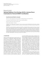
Figure 1 shows the flowchart for music boundary detec-
tion. First, acoustic wave data is transformed into a time-
sequence dataset of feature vectors. The time sequence of
feature vector data is then divided into segments of fixed
length, such as 2 seconds. In the present paper, the term
“segment” stands for this segment of fixed length in the
algorithm called segmental CDP because for each segment,
continuous DP (CDP) is performed. The optimal path of
each segment is searched on the subsequent acoustic data
in order to obtain candidates of similar segment pairs.
The details of the algorithm are described in Section 2.1.
According to the results of segmental CDP, candidates for
similar segment pairs are selected according to the matching
score of segmental CDP. The similar segment pairs are used
to determine music boundaries. Any segment between a pair
of similar segments can be conside red to fall within the
same music piece. This information is transformed into a
histogram of the occurrence of similar segment pairs. Peaks
in the histogram represent the location and the block of each
music piece. The music boundaries are then determined by
extracting both edges of the peaks. The details of determining
music boundaries are described in Section 2.2.
2.2. Segmental CDP for extracting similar
segment pairs

This section describes the algorithm of segmental CDP
for extracting similar segment pairs from a time-sequence
Yoshiaki Itoh et al. 3
dataset. Segmental CDP was developed by improving the
conventional CDP algorithm that efficiently searches for
reference data of a fixed length in long input time-sequence
data. CDP is a type of edge-free dynamic programming that
was originally developed for keyword spotting in speech
recognition. The reference data are composed of feature
vector time-sequence data that are obtained from spoken
keywords. CDP efficiently searches for the reference keyword
in long-speech datasets.
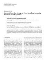
The process of Segmental CDP is explained along with
Figure 2. The horizontal axis represents an input of a feature
vector time-sequence dataset. Segments that are composed
from the same data are plotted on the vertical axis with the
progress of input.
First, segments are composed of the feature vector time-
sequence data. Each segment has a fixed length (N
CDP
frames). The first segment P
1
is composed of the first N
CDP
frames with the progress of input data, as shown by (I) in
Figure 2. With the progress of N
CDP
frames, a new segment
is composed of the newest N
CDP

input frames. As soon
as the new segment is constructed, CDP is performed for
the segment and all other previously constructed segments
toward the subsequent data, as shown by (II) and (III) in
Figure 2.
The optimal path is obtained for each segment at each
time. When a segment P
i
matches an input segment (t
a
, t
b
),
the segments are considered to be similar, as depicted by the
black line in Figure 2. Section (t
a
, t
b
) and segment P
i
(N
CDP
×
(i − 1) + 1, N
CDP
×i) constitute a similar segment pair.
Initially, τ (1
≤ τ ≤ N
CDP
) corresponds to the current

frame on the vertical axis in segment i (1
≤ i ≤ Ns);
and t (1
≤ t ≤ T) corresponds to the current time on
the horizontal axis. N
CDP
, Ns,andT represent the frame
number of a segment, the total number of segments, and
the total number of input frames, respectively. The core
algorithm of Segmental CDP is shown in Algorithm 1.
After N
CDP
frames are input from the beginning, the
first segment is generated and starts computing (a). After all
N
CDP
frames are input, a new segment is generated and starts
computation. Therefore, t/N
CDP
segments are generated in
input time t, discarding the remainder.
Equation (a) computes the local distance between the
feature vectors of the frame τ of segment i and the current
input time t. The cepstral distance or Euclidean distance, for
example, can be used as the local distance.
The three terms of P in (b) represent the cumulative
distances from the three start points, as shown on the right
side of Figure 2. An optimal path is determined according
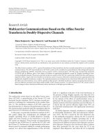
to (c). Here, unsymmetrical local restriction is used because
the computation of (c) is simplified. When the symmetrical

local restriction is used, as described in Figure 3, the number
of additions for local distances is not the same for all three
paths. As shown in Figure 3, the number of additions for
local distances becomes eight when the upper path is always
selected and four when the lower path is always selected. The
number of additions for local distances must be counted and
saved at all DP points, and the cumulative distance must
be normalized by the number of additions when comparing
three cumulative distances in (c). The unsymmetric al local
(1)
2
1
3
(2)
3
3
(3)
(IV) Some of the optimal
paths correspond to
similar segment pairs
(III) For the segment P
i
,
CDP is performed in
the gray area.
(II) Search starts.
Featurevectortime-sequencedata
(I) New
segment
t

1
t
a
t
b
t
T
t
τ
P
1
P
2
τ
T
τ
1
Feature vector time sequence data
P
1
P
2
P
i
.
.
.
P
i+1
.

.
.
P
Ns
Segment
Figure 2: Segmental CDP and DP local restrictions.
12
34
56
78
(12)
4
3(9)
2(6)
1(3)
(9)
(6)
(2 + 1
= 3)
τ
t
N
CDP
P
i
Figure 3: Number of addition for local distances between the
symmetrical and unsymmetric allocal restrictions.
restriction avoids these computations because the numbers
of additions for local distances become the same for all
three paths, as shown in Figure 3 by the number in parent

heses, and it is sufficient to compare the three cumulative
distances in (c). It is confirmed that the unsymmetrical local
restriction has a performance comparable to that of the
symmetrical local restriction.
The cumulative distance G
i
(t, τ) and the starting point
S
i
(t, τ) are updated by (d) and (e), where S
i
(t, τ)denotes
the start time of segment i up to the τth frame. Starting
point information must be stored and must proceed along
the optimal path in the same way as the cumulative distance.
Since N
CDP
is an important system parameter that
affects the performance, the optimal number for N
CDP
is
investigated experimentally.
The conditions of (f) indicate that the segment (S
i
(t,
N
CDP
), t) and the ith segment P
i
are candidates for a similar

section pair, because the total distance G
i
(t, N
CDP
) falls below
the threshold value TH and the local minimum at the last
frame of segment i. Each segment saves the positions and the
total distance of the candidates in accordance with the rank
of the distance G
i
(t, N
CDP
). Let the number of candidates that
each segment saves be m. As shown, the algorithm can be
processed synchronously with input data.
4 EURASIP Journal on Audio, Speech, and Music Processing
LOOP t (1 ≤ t ≤T): for each current time t,
LOOP i (1
≤ i ≤ t/N
CDP
): for each segments
LOOP τ (1
≤ τ ≤ N
CDP
): for each frame of segment i
(a) D
i
(t,τ) = distance

inp


i ×

N
CDP
−1

+ τ

, inp(t)

(b)
P(1)
= G
i
(t − 2, τ − 1) + 2·D
i
(t − 1, τ)+D
i
(t,τ)
P(2)
= G
i
(t − 1, τ − 1) + 3·D
i
(t,τ)
P(3)
= G
i
(t − 1, τ − 2) + 3·D

i
(t,τ − 1) + 3·D
i
(t,τ)
(c) α
∗
= arg min
(α=1,2,3)
P(α)
(d) G
i
(t,τ) = P

α
∗

(e) S
i
(t,τ) =
⎧
⎪
⎪
⎨
⎪
⎪
⎩
S
i
(t − 2, τ − 1)


α
∗
= 1

S
i
(t − 1, τ − 1)

α
∗
= 2

S
i
(t − 1, τ − 2)

α
∗
= 3

End LOOP τ
at the last frame of segment i
(f) if G
i

t,N
CDP

≤
TH, G

i

t,N
CDP

is the local minimum
(g) Save the location data with G
i
(t,N
CDP
)
Segment (S
i
(t,N
CDP
), t) and the ith Segment P
i
are considered to be
candidates for a similar s ection pair.
End LOOP i
End LOOP t
Algorithm 1: Core algorithm of segmental CDP.
Since a music piece does not usually continue for an
hour, similar parts of a segment need not be searched in data
occurring an hour after the segment. Therefore, the current
part around time t is not similar to segment P
i−U
,where
U is large. At LOOP i of the algorithm of segmental CDP,
the starting segment for CDP can be modified from 1 to

t/N
CDP
− U. This modification leads to decreased searching
space and computation time, as well as spurious similar
segments.
2.3. Music boundary detection
2.3.1. Music b oundary detection from
similar segment pairs
A section appearing between a similar segment pair likely
falls within the same music. This section describes a method
for detecting a music boundary from similar segment pairs
extracted by segmental CDP. The proposed method uses
a histogram that shows the same music probability and is
composed of the four steps listed below. Here, Ns denotes
the number of total segments, as mentioned above.
(i) Extract Ns
×m candidates of similar segment pairs by
Segmental CDP.
(ii) Among the candidates in (a), determine similar
segment pairs by extracting Ns
× n (n ≤ m) pairs that are
of higher rank in terms of total distance.
(iii) Draw a line between the members of each similar
segment pair determined in (b).
(iv) Count the number (frequency) of passing lines
on each segment and compose a histogram, as shown in
Figure 3.
First, a sufficient number of candidates (Ns
× m)of
similar segment pairs are extracted, as explained in the

previous section. Second, similar segment pairs are selected
until the number of candidates becomes Ns
× n (n ≤ m)
according to the rank corresponding to the total distance
of Segmental CDP. Third, after extracting similar segment
pairs in (b) and plotting them on a time axis, a line is drawn
between the members of each similar segment pair, as shown
in Figure 3. Lines are drawn for all similar segment pairs.
Finally, the number (frequency) of passing lines on each
segment is counted, and a histogram is composed based on
these numbers, as shown in Figure 3.
A peak is formed within the same music piece, because
specific melodies are repeated in music and many parts
within the music generate similar segments, as shown in
Figure 3. The dips in the graph are taken as candidates for
music boundaries when music pieces continue, and the flat
low parts in the histogram are regarded as a voice section.
An overlap might occur between two similar segment
pairs when their segments become longer from DP matching.
When composing a histogram, the number of lines for an
overlap segment becomes two, which does not significantly
affect the histogram.
The time difference of a similar segment pair should
be less than one hour, because music pieces usually do not
exceedonehour.Thesearchareacanberestrictedtoafixed
length, such as 5 minutes. Such a restriction can reduce
the number of incorrect similar segment pairs as well as
the computation complexity of segment CDP. For example,
the computation perplexity becomes less than 1/10 when
restricted to 5 minutes for a 90-minute program.

Yoshiaki Itoh et al. 5
Here, m is a parameter that affects the performance, and
the optimal number for n is investigated in the following
experiments.
2.3.2. Introduction of dissimilarity measure for
finding feature vector changing points
In this section, we introduce a dissimilarity measurement
to demonstrate that the proposed method can extract the
location of each music piece.
The starting and ending parts in a music piece are often
unique and are not repeated within the music piece. As a
result, the histogram depicted in Figure 3 is not generated
around the starting and ending parts. The boundaries
detected using similarity in a music piece tend to become the
approximate location. Acoustic feature vectors are thought
to be different at accurate music boundaries. Accurate music
boundaries can be detected by a detailed analysis of the
area around the points that are regarded as the music
boundaries by the music boundary detection using similarity
in a music piece. In order to find acoustically changing points
of the feature vectors, we introduce a simple dissimilarity
measurement expressing the discontinuity of the feature
vectors, as follows:
Dist(t)
=

I
i
=1
distance (t, t − i)

I
,
(1)
D
new

t

+ j

=
⎧
⎪
⎪
⎪
⎪
⎨
⎪
⎪
⎪
⎪
⎩
max
0≤j≤J
Dist

t

+ j


×cos

π
2
·
j
J

at start boundary,
max
0≤j≤J
Dist

t

+ j

×
cos

π
2
·
j
J

at end boundary,
(2)
where Dist(t)in(1) indicates the dissimilarity between the
current frame vector at t and the preceding vectors for I

frames. From the boundary at time t

that is obtained by the
music boundary detection using similarity in a music piece,
an acoustic changing point of the feature vectors is searched
toward the outside of a music piece according to (2). The
point of maximum dissimilarity of D
new
(t

+ j)att

+ j is
regarded as a new music boundary. Here, a cosine window is
used to give a larger weight to the points that are nearer the
first detected boundary at t

. In the following experiments,
a cepstral distance is used for the distance Distance(t, t
− i)
between the frame t vectors and the frame t
− i vectors. The
parameters I and J were determined experimentally to be 10
seconds and 20 seconds, respectively.
3. EVALUATION EXPERIMENTS
3.1. Evaluation data and experimental conditions
Experiments were performed to evaluate the performance
of the proposed method for detecting music boundaries.
The object data in these experiments are popular music data
taken from the open RWC music database [11]. The database

includes 100 popular music pieces. The total length of the
music sets is 6 hours and 38 minutes. The average time is 3
minutes 58 seconds, and the longest and shortest times are 6’
32” and 2’ 12,” respectively.
First, silent parts, which are added before and after
each music piece, are deleted because real-world video data
usually have no boundary information for music. Two types
of datasets were prepared. For the first dataset, a continuous
music dataset was obtained by concatenating 100 music
datasets. Silent parts between music pieces were not included
in the dataset. This condition is considered to be strict for
methods that consider the acoustic difference [4–6]. There
were 99 boundaries for the continuous music dataset. For
the second dataset, a music-voice mixed dataset, in which a
one-minute speech was inserted between music pieces, was
used as the continuous music dataset. Therefore, we inserted
99 speech sections that were taken from an open speech
corpus of Japanese newspaper article sentences. There were
198 boundaries between voice sections and music sections.
The music data were sampled at 44.1 kHz in stereo and
were quantized at 16 bits. A 20D mel-frequency cepstral
coefficient [12] was used as a feature vector. Cepstral distance
was used as the local distance in (a). The window size for
analysis and the frame shift were both 46 milliseconds (2,048
samples).
This method employs two main parameters. The first is
the segment length N
CDP
in segment CDP, and the second
is the number of similar segment pairs Ns

× n in (b) of
Section 2.3. We performed an experiment while varying the
parameters N
CDP
and Ns× n, as shown below:
(i) segment length: N
CDP
= 21,42, 63 frames (1.0, 2.0,
3.0, 4.0, 5.0 seconds),
(ii) number of similar segment pairs: n
= 0.5, 1.0, 2.0,
3.0, 5.0.
In the experiment, the search area for similar segment
pairs was restricted to 5 minutes.
For evaluation measurement, we used precision rate,
recall rate, and F-measure, which are general measurements
for retrieval tasks, as shown in the following equations:
precision rate
=
correctly detected boundaries
detected boundaries
,
(3)
recall rate
=
correctly detected boundaries
actual boundaries
,(4)
F-measure
=

recall × precision
(recall + precision)/2
. (5)
3.2. Results and discussion
3.2.1. Evaluation of system parameters
Under the conditions mentioned above, experiments are
conducted for the purpose of detecting music boundaries
among 100 music pieces.
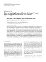
Figure 4 shows the representative results for the continu-
ous music dataset, where the segment length is N
CDP
= 21
frames (1.0 s) and the number of similar segment pairs is
6 EURASIP Journal on Audio, Speech, and Music Processing
(2) Extracted similar section pairs (3) Draw line between members
(4) Count the number of lines by (3)
Time
Music boundary
Frequency
Figure 4: Composing a histogram expressing music piece loca-
tions.
5000 6000 7000 8000 9000 10000
Time
0
100
200
300
Frequency
Figure 5: Frequency contour of similar segment pairs along a time
axis. Each vertical line in the figure represents actual boundaries.

Ns × n = 21, 768 (Ns = 21, 768, n = 1.0). Figure 4 shows
the frequency contour of similar segment pairs along a time
axis, according to Section 2.3. Each vertical line in the figure
represents the actual boundaries. We confirmed that dips in
the graph appear near the music boundaries.
(1) Evaluation for segment length N
CDP
Figure 5 shows the overall performance obtained by varying
the segment length N
CDP
, where the precision rate and recall
rate are used for measurement. The detected boundary is
conside red to be correct if the boundary falls within 5
seconds of the actual boundary. The best performance is
obtained under the condition shown in Figure 4 [N
CDP
= 21
frames (1.0 s), Ns
× n = 21,768 (Ns = 21, 768, n = 1.0)].
The point X on the line indicates that 80% of boundaries
are correct (recall rate) when 112 boundary candidates are
extracted (70% precision rate) by this method. The best F-
measure, defined as a harmonic average of the precision and
recall rate, becomes 0.74.
The performance decreases when N
CDP
exceeds 2 sec-
onds, as shown in Figure 5. The reason for this is assumed
to be that correct similar segment pairs decrease and the
0

20
40
60
80
100
Recall rate (%)
0 20 40 60 80 100
Precision rate (%)
N
= 10 (0.5s)
N
= 21 (1 s)
N
= 42 (2 s)
N
= 63 (3 s)
Figure 6: Music boundary detection performance according to
segment length N
CDP
(N= N
CDP
in the figure).
peak shown in Figure 4 cannot be formed. Meanwhile, short
segments cause performance deterioration, because of an
increase in false matching between other music pieces. The
best performance was obtained at a segment length of 1
second for the datasets.
(2) Evaluation of the number of candidates Ns
×n
Figure 6 shows the overall performance for various numbers

of candidates Ns
× n. The performance deteriorates when
the number of candidates n is small. The reason for this is
assumed to be that the number of similar segment pairs is
insufficient to form the correct peaks. Meanwhile, incorrect
similar segment pairs are generated when the number is
large. The best performance is obtained at the same number
of segments, n
= 1.0 for the datasets.
(3) Evaluation of DP and linear matching
Figure 7 shows the results of linear matching compared to DP
matching. Linear matching can be performed with a slight
modification of the segment CDP algorithm, as described
in Section 2.2. The DP restriction in Figure 1 is limited to
the center path only, and (f) through (4)arecomputedat
α
= α
∗
= 2. The performance of linear matching is slightly
better than that of DP matching. Since repeated sections of
music in the experiments are not lengthened or shortened
and are of approximately the same length, the peaks in the
music sections are correctly formed in linear matching. The
method using DP matching is expected to work well for
speech datasets because nonlinear matching is necessary for
speech data.
Yoshiaki Itoh et al. 7
0
20
40

60
80
100
Recall rate (%)
0 20 40 60 80 100
Precision rate (%)
n
= 0.5
n
= 1
n
= 2
n
= 3
n
= 5
Figure 7: Music boundary detection performance according to the
number of candidates and comparison with linear matching.
0
20
40
60
80
100
Recall rate (%)
0 20 40 60 80 100
Precision rate (%)
DP
Linear
Figure 8: Music boundary detection performance comparison

between DP matching and linear matching.
0
20
40
60
80
100
Recall rate (%)
0 20 40 60 80 100
Precision rate (%)
Continuous music data
Voice-music mixed data
Figure 9: Music boundary detection performance for a voice-music
mixed dataset.
0
20
40
60
80
100
Recall rate (%)
0 20 40 60 80 100
Precision rate (%)
Dissimilarity
Similarity
Figure 10: Comparison of music boundary detection performance
for a continuous music dataset and a voice-music mixed dataset.
8 EURASIP Journal on Audio, Speech, and Music Processing
0
20

40
60
80
100
Recall rate (%)
0 20 40 60 80 100
Precision rate (%)
Dissimilarity
Similarity
Figure 11: Performance improvement by introducing dissimilarity
measure for a voice-music mixed dataset.
3.2.2. Evaluation of voice-music mixed dataset
Music boundary detection performance was evaluated for
a voice-music mixed dataset. Figure 8 shows the obtained
results, where the segment length was N
CDP
= 21 frames
(1.0 s) and the number of similar segment pairs was n
=
1.0. The performance deteriorates for the mixed dataset,
although peaks were formed, as shown in Figure 4.Theper-
formance deterioration occurred for the following reason.
Since the beginning and end of a music piece tend to be
similar, peaks were not formed at the beginning or end of
music pieces. Since the peaks are formed in the frequency
contour and the rough location of each music piece was
identified by the method, a detailed detection method is
required. We, hereby, introduce a simple detection method
by finding acoustically changing points of the feature vectors.
In the next section, this method is described briefly, and

we confirm that the proposed method works well for music
boundary detection from similarity in a music piece.
3.2.3. Evaluation of introducing dissimilarity measure
Music boundary detection performance by introducing
a dissimilarity measure for finding acoustically changing
points was evaluated for both a voice-music mixed dataset
and a continuous music dataset. Figure 9 shows the results of
using dissimilarity of feature vectors for a voice-music mixed
dataset. The performance for music boundary detection was
greatly improved. Figure 10 also shows the results obtained
using dissimilarity of feature vectors for a continuous music
dataset. Again, the performance was also improved. These
0
20
40
60
80
100
Recall rate (%)
0 20 40 60 80 100
Precision rate (%)
5s
4s
3s
2s
1s
Figure 12: Performance improvement by introducing dissimilarity
measure for a continuous music dataset.
results indicate that the proposed method using similarity in
music piece worked well for roughly identifying where each

music piece is located in the acoustical dataset, and a detailed
analysis around the detected boundaries is needed to obtain
accurate boundaries.
3.2.4. Evaluation of correct range of music boundaries
As mentioned at (a) in Section 3.2.1, the detected boundary
is considered to be correct if the boundary falls within 5
seconds of the actual boundary. Since this criterion, referred
to herein as the correct range, is thought not to be severe, we
performed an experiment while varying the correct range.
The results are shown in Figure 11, and the performance
declined significantly. When the correct range is 2 seconds
from an actual music boundary, the precision and the recall
rates become less than 30%, and the system does not seem
to be feasible. The reason for this is thought to be the
same as that described in the previous section. Although
the proposed method using similarity in music piece could
roughly identify the location of each music piece, it is
necessary to identify the music boundaries precisely.
Figure 12 shows the results when varying the correct
range from 1 second to 5 seconds. The performance for
music boundary detection did not deteriorate compared
with that shown in Figure 11 because the accurate bound-
aries are identified by extracting the changing points of fea-
ture vectors. Figure 13 shows the music boundary detection
performance according to the correct range for a continuous
music dataset. The performance was also improved.
Yoshiaki Itoh et al. 9
0
20
40

60
80
100
Recall rate (%)
0 20 40 60 80 100
Precision rate (%)
5s
4s
3s
2s
1s
Figure 13: Music boundary detection performance according to the
correct range for a voice-music mixed dataset.
We obtained an F-measure of 0.84 for a continuous
music dataset and an F-measure of 0.74 for a voice-music
mixed dataset.
3.2.5. Experiment for an actual music program
We applied the proposed method to an actual broadcasted
music program, which was recorded by videotape, and
converted the program into digital data on a computer. The
data format and experimental conditions were the same
as those described in Section 3.1 (N
CDP
= 21 frames = 1
second, n
= 1.0). Figure 14 shows the obtained results. The
horizontal axis and vertical axes indicate the input time and
the frequency of passing lines, respectively. The graph shows
the results for 15 minutes. The program consisted of three
music pieces, and three peaks are formed for each music

piece. There were no oversegmentation within music pieces.
The section from segment 420 to segment 740 was flat,
because the conversation continued during this section. The
boundaries detected by the proposed method were located
within 5 seconds of the actual boundaries. Thus, the results
indicate that the proposed method works well for real-world
music data.
3.2.6. Future research
The method described in Section 3.2.3 using a dissimilarity
measure is thought to be a nonoptimal method for finding
feature vector changing points. Therefore, we sought an
optimal method using Gaussian mixture models (GMM), a
support vector machine, and so on. Throughout the experi-
0
20
40
60
80
100
Recall rate (%)
0 20 40 60 80 100
Precision rate (%)
1s
2s
3s
4s
5s
Figure 14: Music boundary detection performance according to the
correct range for a continuous music dataset.
0 200 400 600 800 1000

Segment
0
50
100
150
200
250
Frequency
Figure 15: Frequency contour of similar segment pairs for music
pieces and speech datasets using an actual music television pro-
gram.
ments of the present study, the optimal parameters, such as
N
CDP
and n, were obtained for the closed datasets. Therefore,
the robustness of the parameters must be evaluated using
various types of datasets. For example, the tempos of each
music piece are different, and a suitable value of N
CDP
is
thought to exist for each tempo. A method is needed for
adapting N
CDP
to each music piece according to its tempo
and other parameters. The proposed algorithm deals with
the monotonic similarity of a constant length of segments,
and does not take into account the hierarchical structure of
a music piece. A more elaborate algorithm should also be a
topic of future studies to discuss hierarchical similarity in a
music piece.

10 EURASIP Journal on Audio, Speech, and Music Processing
Music is not only based on “repetition,” but also on
“variation,” such as in modulation and different verses
that might deteriorate the performance of the algorithm.
The present study focused on popular music that is most
frequently broadcasted in TV programs. The algorithm
should also be evaluated using other music genres such as
jazz and lyrics in a future study. We have already quantified
the proposed method using pseudomusic datasets, and the
next step will be to apply it to real-world streaming data, such
as the music program described in Section 3.2.5.
4. CONCLUSIONS
The present paper proposed a new approach for detecting
music boundaries in a music stream dataset. The proposed
method extracts similar segment pairs in a music piece
by segmental continuous dynamic programming and can
identify the location of each music piece according to
the information of occurrence positions of the similar
segment pairs. The music boundaries are then determined.
Experimental results reveal that the proposed approach is a
promising method for detecting music boundaries between
music pieces, while avoiding oversegmentation within music
pieces. An optimal method for finding the acoustic changing
points using GMM, and so on, will be studied in the future.
Better parameter sets (feature vector, number of frame shift,
etc.) must be investigated for this purpose. Evaluation should
be performed using other music genres and real-world
stream data, such as video data, because the experiments of
the present study examined only the popular music genre
and speech corpus data.

ACKNOWLEDGMENTS
This research was supported in part by Grant-in-Aid for
Scientific Research (C) no. KAKENHI 1750073 and Iwate
Prefectural Foundation.
REFERENCES
[1] Y. Itoh and K. Tanaka, “A matching algorithm between arbi-
trary sections of two speech data sets for speech retrieval,” in
Proceedings of the IEEE International Conference on Acoustics,
Speech and Signal Processing (ICASSP ’01), vol. 1, pp. 593–596,
Salt Lake City, Utah, USA, May 2001.
[2] J. Kiyama, Y. Itoh, and R. Oka, “Automatic detection of topic
boundaries and keywords in arbitrary speech using incremen-
tal reference interval-free continuous DP,” in Proceedings of
the 4th International Conference on Spoken Language Processing
(ICSLP ’96), vol. 3, pp. 1946–1949, Philadelphia, Pa, USA,
October 1996.
[3] G. Smith, H. Murase, and K. Kashino, “Quick audio retrieval
using active search,” in Proceedings of the IEEE Interna-
tional Conference on Acoustics, Speech and Signal Processing
(ICASSP ’98), vol. 6, pp. 3777–3780, Seattler, Wash, USA, May
1998.
[4] M. Cooper and J. Foote, “Automatic music summarization
via similarity analysis,” in Proceedings of the 3rd International
Conference on Music Information Retrieval (ISMIR ’02),pp.
81–85, Paris, France, October 2002.
[5] J. Foote, “Automatic audio segmentation using a measure
of audio novelty,” in Proceedings of the IEEE International
Conference on Multimedia and Expo (ICME ’00), vol. 1, pp.
452–455, New York, NY, USA, July-August 2000.
[6] E. Allamanche, J. Herre, O. Hellmuth, T. Kastner, and

C. Ertel, “A multiple feature model for musical similarity
retrieval,” in Proceedings of the 4th International Conference on
Music Information Retrieval (ISMIR ’03),Baltimore,Md,USA,
October 2003.
[7] M. J. Carey, E. S. Parris, and H. Lloyd-Thomas, “A comparison
of features for speech, music discrimination,” in Proceedings
of the IEEE International Conference on Acoustics, Speech and
Signal Processing (ICASSP ’99), vol. 1, pp. 149–152, Phoenix,
Ariz, USA, March 1999.
[8] K. El-Maleh, M. Klein, G. Petrucci, and P. Kabal, “Speech/
music discrimination for multimedia applications,” in Pro -
ceedings of the IEEE International Conference on Acoustics,
Speech and Signal Processing (ICASSP ’00), vol. 4, pp. 2445–
2448, Istanbul, Turkey, June 2000.
[9] J. Saunders, “Real-time discrimination of broadcast speech/
music,” in Proceedings of the IEEE International Conference on
Acoustics, Speech and Signal Processing (ICASSP ’96), vol. 2, pp.
993–996, Atlanta, Ga, USA, May 1996.
[10] M. M. Goodwin and J. Laroche, “A dynamic programming
approach to audio segmentation and speech/music discrimi-
nation,” in Proceedings of the IEEE International Conference on
Acoustics, Speech and Signal Processing (ICASSP ’04), vol. 4, pp.
309–312, Montreal, Canada, May 2004.
[11] M. Goto, H. Hashiguchi, T. Nishimura, and R. Oka, “RWC
music database: popular, classical, and jazz music databases,”
in Proceedings of the 3rd International Conference on Music
Information Retrieval (ISMIR ’02), Paris, France, October
2002.
[12] L. Rabiner and B. H. Juang, Fundamentals of Speech Recogni-
tion, Prentice-Hall, Englewood Cliffs, NJ, USA, 1993.