Báo cáo hóa học: " Research Article Efficient Adaptive Combination of Histograms for Real-Time Tracking" pdf

Hindawi Publishing Corporation
EURASIP Journal on Image and Video Processing
Volume 2008, Article ID 528297, 11 pages
doi:10.1155/2008/528297
Research Article
Efficient Adaptive Combination of Histograms for
Real-Time Tracking
F. Bajramovic,
1
B. Deutsch,
2
Ch. Gr
¨
aßl,
2
and J. Denzler
1
1
Department of Mathematics and Computer Science, Friedrich-Schiller University Jena, 07737 Jena, Germany
2
Computer Science Department 5, University of Erlangen-Nuremberg, 91058 Erlangen , Germany
Correspondence should be addressed to F. Bajramovic,
Received 30 October 2007; Revised 14 March 2008; Accepted 12 July 2008
Recommended by Fatih Porikli
We quantitatively compare two template-based tracking algorithms, Hager’s method and the hyperplane tracker, and three
histogram-based methods, the mean-shift tracker, two trust-region trackers, and the CONDENSATION tracker. We perform
systematic experiments on large test sequences available to the public. As a second contribution, we present an extension to the
promising first two histogram-based trackers: a framework which uses a weighted combination of more than one feature histogram
for tracking. We also suggest three weight adaptation mechanisms, which adjust the feature weights during tracking. The resulting
new algorithms are included in the quantitative evaluation. All algorithms are able to track a moving object on moving background
in real time on standard PC hardware.

Copyright © 2008 F. Bajramovic et al. This is an open access article distributed under the Creative Commons Attribution License,
which permits unrestricted use, distribution, and reproduction in any medium, provided the original work is properly cited.
1. INTRODUCTION
Data driven, real-time object tracking, is still an important
and in general unsolved problem with respect to robustness
in natural scenes. For many high-level tasks in computer
vision, it is necessary to track a moving object—in many
cases on moving background—in real time without having
specific knowledge about its 2D or 3D structure. Exam-
ples are surveillance tasks, action recognition, navigation
of autonomous robots, and so forth. Usually, tracking is
initialized based on change detection in the scene. From this
moment on, the position of the moving target is identified in
each consecutive frame.
Recently, two promising classes of 2D data-driven track-
ing methods have been proposed: template- (or region-)
based tracking methods and histogram-based methods. The
idea of template-based tracking consists of defining a region
of pixels belonging to the object and using local optimization
methods to estimate the transformation parameters of the
region between two consecutive images. Histogram-based
methods represent the object by a distinctive histogram,
for example, a color histogram. They perform tracking by
searching for a region in the image whose histogram best
matches the object histogram from the first image. The
search is typically formulated as a nonlinear optimization
problem.
As the first contribution of this paper, we present a
comparative evaluation (previously published at a confer-
ence [1]) of five different object trackers, two template-

based [2, 3] and three histogram-based approaches [4–6]. We
test the performance of each tracker with pure translation
estimation, as well as with translation and scale estimation.
Due to the rotational invariance of the histogram-based
methods, further motion models, such as rotation or general
affine motion, are not considered. In the evaluation, we focus
especially on natural scenes with changing illuminations and
partial occlusions based on a publicly available dataset [7].
The second contribution of this paper concentrates on
the promising class of histogram-based methods. We present
an extension of the mean-shift and trust-region trackers,
which allows using a weighted combination of several dif-
ferent histograms (previously published at a conference [8]).
We refer to this new tracker as combined histogram tracker
(CHT). We formulate the tracking optimization problem in
a general way such that the mean-shift [9]aswellasthe
trust-region [10] optimization can be applied. This allows
for a maximally flexible choice of the parameters which
2 EURASIP Journal on Image and Video Processing
are estimated during tracking, for example, translation, and
scale.
We also suggest three different online weight adaptation
mechanisms for the CHT, which automatically adapt the
weights of the individual features during tracking. We
compare the CHT (with and without weight adaptation)
with histogram trackers using only one specific histogram.
The results show that the CHT with constant weights can
improve the tracking performance when good weights are
chosen. The CHT with weight adaptation gives good results
without a need for a good choice for the right feature or

optimal feature weights. All algorithms run in real time (up
to 1000 frames per second excluding IO).
The paper is structured as follows: In Section 2,wegive
a short introduction to template-based tracking. Section 3
gives a more detailed description of histogram-based trackers
and shows how two suitable local optimization methods, the
mean-shift and trust-region algorithms, can be applied. In
Sections 4 and 5, we present the main algorithmic contri-
butions of the paper: a rigorous mathematical description
for the CHT followed by the weight adaptation mechanisms.
Section 6 presents the experiments: we first describe the test
set and evaluation criteria we use for our comparative study.
The main comparative contribution of the paper consists
of the evaluation of the different tracking algorithms in
Section 6.2. In Sections 6.3 and 6.4, we present the results for
the CHT and the weight adaptation mechanisms. The paper
concludes with a discussion and an outlook to future work.
2. REGION-BASED OBJECT TRACKING
USING TEMPLATES
One class of data driven object tracking algorithms is based
on template matching. The object to be tracked is defined
by a reference region r
= (u
1
, u
2
, , u
M
)
T

in the first image.
The gray-level intensity of a point u at time t is given by
f (u, t). Accordingly, the vector f(r, t) contains the intensities
of the entire region r at time t and is called template. During
initialization, the reference template f(r,0) isextracted from
the first image.
Template matching is performed by computing the
motion parameters µ(t) which minimize the squared inten-
sity differences between the reference template and the
current template:
µ(t)
= argmin
size µ


f(r,0)−f(g(r, µ),t)


2
. (1)
The function g(r, µ) defines a geometric transformation of
the region, parameterized by the vector µ.Severalsuch
transformations can be considered, for example, Jurie and
Dhome [3] use translation, rotation, and scale, but also affine
and projective transformations. In this paper, we restrict
ourselves to translation and scale estimation.
A brute-force search minimization of (1) is computa-
tionally expensive. It is more efficient to approximate µ
through a linear system:
µ(t +1)= µ(t)+A(t +1)


f(r,0)−f

g(r, µ(t)

, t +1)

.
(2)
For detailed background information on this class of tracking
approaches, the reader is referred to [11].
We compare two approaches for computing the matrix
A(t +1)in(2). Jurie and Dhome [3] perform a short training
step, which consists of simulating random transformations
of the reference template. The resulting tracker will be
called hyperplane tracker in our experiments. Typically,
around 1000 transformations are executed and their motion
parameters
µ
i
and difference vectors f(r,0) − f(g(r, µ
i
), 0)
are collected. Afterwards, the matrix A is derived through
a least squares approach. Note that this allows making A
independent of t. For details, we refer to the original paper.
Hager and Belhumeur [2] propose a more analytical
approach based on a first-order Taylor approximation.
During initialization, the gradients of the region points are
calculated and used to build a Jacobian matrix. Although A

cannot be made independent of t, the transformation can
be performed very efficiently and the approach has real-time
capability.
3. REGION-BASED OBJECT TRACKING
USING HISTOGRAMS
3.1. Representation and tracking
Another type of data driven tracking algorithms is based on
histograms. As before, the object is defined by a reference
region, which we denote by R(x(t)), where x(t) contains
the time variant parameters of the region, also referred
to as the state of the region. Note that R(x(t)) is similar,
but not identical, to g(r, µ(t)). The later transforms a set
of pixel coordinates to a set of (sub)pixel coordinates,
while the former defines a region in the plane, which is
implicitly treated as the set of pixel coordinates within
that region. This implies that R(x(t)) does not contain any
subpixel coordinates. One simple example for a region is a
rectangle of fixed dimensions. The state of the region x(t)
=
(m
x
(t), m
y
(t))
T
is the center of the rectangle in (sub)pixel
coordinates m
x
(t)andm
y

(t)foreachtimestept. With this
simple model, tracking the translation of a region can be
described as estimating x(t) over time. If the size of the region
is also included in the state, estimating the scale will also be
possible.
The information contained within the reference region
is used to model the moving object. The information
may consist of the color, the gray value, or certain other
features, like the gradient. At each time step t and for
each state x(t), the representation of the moving object
consists of a probability density function p(x(t)) of the
chosen features within the region R(x(t)). In practice, this
density function has to be estimated from image data.
For performance reasons, a weighted histogram q(x(t))
=
(q
1
(x(t)), q
2
(x(t)), , q
N
(x(t)))
T
of N bins q
i
(x(t)) is used
as a nonparametric estimate of the true density, although it is
well known that this is not the best choice from a theoretical
point of view [12]. Each individual bin q
i

(x(t)) is computed
by
q
i

x(t)

=
C
x(t)

u∈R(x(t))
L
x(t)
(u)δ

b
t
(u) −i

, i = 1, , N,
(3)
F. Bajramovic et al. 3
where L
x(t)
(u) is a suited weighting function, which will
be introduced below, b
t
is a function which maps the
pixel coordinate u to the bin index b

t
(u) ∈{1, , N}
according to the feature at position u,andδ is the Kronecker-
Delta function. The value C
x(t)
= 1/

u∈R(x(t))
L
x(t)
(u)is
a normalizing constant. In other words, (3)countsall
occurrences of pixels that fall into bin i, where the increment
within the sum is given by the weighting function L
x(t)
(u).
Object tracking can now be defined as an optimization
problem. We initially extract the reference histogram q(x(0))
from the reference region R(x(0)). For t>0, the tracking
problem is defined by
x(t)
= argmin
x
D

q

x(0)

, q(x)


,(4)
where D(
·, ·) is a suitable distance function defined on
histograms. We use three local optimization techniques:
the mean-shift algorithm [4, 9], a second-order trust-region
algorithm [5, 10] (referred to simply as the trust-region
tracker), and also a simple first-order trust-region variant
[13] (called first-order trust-region tracker or trust-region
1st for short), which can be considered as gradient descent
with online step size adaptation. It is also possible to apply
quasiglobal optimization using a particle filter and the
CONDENSATION algorithm as suggested by P
´
erez et al. [6],
and Isard and Blake [14].
3.2. Kernel and distance functions
There are two open aspects left: the choice of the weighting
function L
x(t)
(u)in(3) and the distance function D(·, ·). The
weighting function is typically chosen as an elliptic kernel,
whose support is exactly the region R(x(t)), which thus has
to be an ellipse. Different kernel profiles can be used, for
example, the Epanechnikov, the biweight, or the truncated
Gaussprofile[13].
For the optimization problem in (4), several distance
functions on histograms have been proposed, for example,
the Bhattacharyya distance, the Kullback-Leibler distance,
the Euclidean distance, and calar product-based distance. It

is worth noting that for the following optimization no metric
is necessary. The main restriction on the given distance
functions in our work is the following special form
D

q

x(0)

, q(x)

=

D

N

n=1
d

q
n

x(0)

, q
n
(x)



(5)
with a monotonic, bijective function

D,andafunction
d(a,b), which is twice differentiable with respect to b.By
substituting (5) into (4), we get
x(t)
= argmax
x
− S(x)
(6)
with S(x)
= sgn(

D)
N

n=1
d

q
n

x(0)

, q
n
(x)

,

(7)
where sgn(

D) = 1if

D is monotonically increasing, and
sgn(

D) =−1if

D is monotonically decreasing. More details
can be found in [13]. The following subsections deal with the
optimization of (6) using the mean-shift algorithm as well as
trust-region optimization.
3.3. Mean-shift optimization
The main idea for the derivation of the mean-shift tracker
consists of a first-order Taylor approximation of the mapping
q(x)
→−S(x)atq(x), where x is the estimate for x(t)from
the previous mean-shift iteration (in the first iteration, the
result from frame t
−1 is used instead). Furthermore, the state
x has to be restricted to the position of the moving object in
the image plane (tracking of position only). After a couple of
computations and simplifications (for details, see [13]), we
get
x(t)
≈ argmax
x


C
0

u∈R(x)
L
x
(u)
N

n=1
δ

b
t
(u) −n

w
t
(x, n)

=
argmax
x

C
0

u∈R(x)
L
x

(u) w
t


x, b
t
(u)


(8)
with the weights
w
t
(x, n) =−sgn(

D)
∂d(a,b)
∂b




(a,b)=(q
n
(x(0)),q
n
(x))
. (9)
This special reformulation allows us to interpret the weights
w

t
(x, b
t
(u)) as weights on the pixel coordinate u.The
constant C
0
can be shown to be independent of x. Finally, we
can apply the mean-shift algorithm for the optimization of
(8), as it is a weighted kernel density estimate. It is important
to note that scale estimation cannot be integrated into the
mean-shift optimization. To compensate for this, a heuristic
scale adaptation can be applied, which runs the optimization
threetimeswithdifferent scales. Further details can be found
in [4, 13, 15].
3.4. Trust-region optimization
Alternatively, a trust-region algorithm can be applied to
the optimization problem in (4). In this case, we need
the gradient and the Hessian (only for the second-order
algorithm) of S(x):
∂S(x)
∂x
,
∂
2
S(x)
∂x∂x
. (10)
Both quantities can be derived in closed form. Due to lack of
space, only the beginning of the derivation is given and the
reader is referred to [13],

∂S(x)
∂x
i
=
N

n=1
∂S(x)
∂q
n
(x)
∂q
n
(x)
∂x
i
=
N

n=1
− w
t
(x, n)
∂q
n
(x)
∂x
i
.
(11)

Note that the expression
w
t
(x, n) from the derivation of the
mean-shift tracker in (9) is also required for the gradient and
the Hessian (after replacing
x by x). As for the mean-shift
tracker, after further reformulation this expression changes
into the pixel weights
w
t
(x, b
t
(u)) (again with x instead of
x). The advantage of the trust-region method consists of
the ability to integrate scale and rotation estimation into the
optimization problem [5, 13].
4 EURASIP Journal on Image and Video Processing
3.5. Example for mean-shift tracker
We give an example for the equations and quantities
presented above. Using the Bhattacharyya distance between
histograms (as in [4]),
D

q

x(0)

, q


x(t)

=

1 −B

q

x(0)

, q

x(t)

(12)
with
B

q

x(0)

, q

x(t)

=
N

n=1


q
n

x(0)

·
q
n

x(t)

, (13)
we have

D(a) =
√
1 −a, d(a, b) =
√
a·b,and
w
t
(n) =
1
2




q

n

x(0)

q
n

x(t)

. (14)
4. COMBINATION OF HISTOGRAMS
Up to now, the formulation of histogram-based tracking
uses the histogram of a certain feature, defined a priori
for the tracking task at hand. Examples are gray value
histograms, gradient strength (edge) histograms, and RGB
or HSV color histograms. Certainly, using several different
features for representing the object to be tracked will result
in better tracking performance, especially if the different
features are weighted dynamically according to the situation
in the scene. For example, a color histogram may perform
badly, if illumination changes. In this case, information on
the edges might be more useful. On the other hand, in case of
a uniquely colored object in a highly textured environment,
color is preferable over edges.
It is possible to combine several features by using
one high-dimensional histogram. The problem with this
approach is the curse of dimensionality; high-dimensional
features result in very sparse histograms and thus a very
inaccurate estimate of the true and underlying density.
Instead, we propose a different solution for combining

different features for object tracking. The key idea is to
use a weighted combination of several low-dimensional
(weighted) histograms. Let H
={1, , H} be the set of
features used for representing the object. For each feature
h
∈ H , we define a separate function b
(h)
t
(u). The number
of bins in histogram h is N
h
and may differ between the
histograms. Also, for each histogram, a different weighting
function L
(h)
x(t)
(u) can be applied, that is, different kernels
for each individual histogram are possible if necessary. This
results in H different weighted histograms q
(h)
(x(t)) with the
bins
q
(h)
i

x(t)

= C

(h)
x(t)

u∈R(x(t))
L
(h)
x(t)
(u)δ

b
(h)
t
(u) −i

,
h
∈ H , i = 1, , N
h
.
(15)
We now define a combined representation of the object
by φ(x(t))
= (q
(h)
(x(t)))
h∈H
and a new distance function
(compare (4)and(5)), based on the weighted sum of the
distances for the individual histograms,
D

∗
(x) =

h∈H
β
h
D
h

q
(h)

x(0)

, q
(h)

x(t)

, (16)
where β
h
≥ 0 is the contribution of the individual histogram
h to the object representation. The quantities β
h
can be
adjusted to best model the object in the current context
of tracking. In Section 5, we will present a mechanism
for online adaptation of the feature weights. Alternatively,
instead of the linear combination D

∗
(x) of the distances
D
h
(q
(h)
(x(0)), q
(h)
(x(t))), a linear combination of the sim-
plified expressions S
h
(x) (straight forward generalization of
(7)) can be used as follows:
S
∗
(x) =

h∈H
β
h
S
h

x(t)

. (17)
In the single histogram case, minimizing D(q(x(0)), q(x(t)))
is equivalent to minimizing S(x). In the combined histogram
case, however, the equivalence of minimizing D
∗

(x)and
S
∗
(x) can only be guaranteed, if

D
h
(a) =±a for all h ∈ H .
Nevertheless, S
∗
(x) can still be used as an objective function,
if this condition is not fulfilled. Because of its simpler form
and the lack of obvious advantages of D
∗
(x), we choose the
following optimization problem for the combined histogram
tracker:
x(t)
= argmax
x
S
∗
(x). (18)
From a theoretical point of view, using the simplified
objective function S
∗
is equivalent to restricting the class
of distance measures D
h
for each feature h to those that

fulfill

D
h
(a) =±a (as in this case D
h
= S
h
). For example,
this excludes the Euclidean distance, but does allow for the
squared Euclidean distance.
4.1. Mean-shift optimization
For the mean-shift tracker, we have to use the same weighting
function L
x(t)
(u) for all histograms h and again the state x
has to be restricted to the position of the moving object in
the image plane. After a technically somewhat tricky, but
conceptually straight forward extension of the derivation for
the single histogram mean-shift tracker, we get
x(t)
≈ argmax
x
C
0

u∈R(x)
L
x
(u)


h∈H
w
h,t

x, b
(h)
t
(u)

,
  
:=w
t
(x,u)
(19)
which is again a weighted kernel density estimate. The
corresponding pixel weights are
w
t
(x, u) =

h∈H
w
h,t


x, b
(h)
t

(u)

=

h∈H
− β
h
sgn

D
h

∂d
h
(a, b)
∂b




(a,b)=(q
(h)
b
t
(u)
(x(0)),q
(h)
b
t
(u)

(x))
,
(20)
where d
h
(a, b)isdefinedasin(5) for each individual
feature h.
F. Bajramovic et al. 5
0
20
40
60
80
e
c
00.20.40.60.8
Quantile
Hager
Hyperplane
CONDENSATION
Tr us t re g io n
Tr us t re g io n 1st
Mean shift
(a)
0
20
40
60
80
e

c
00.20.40.60.8
Quantile
Hager
Hyperplane
CONDENSATION
Tr us t re g io n
Tr us t re g io n 1st
Mean shift
(b)
0
0.2
0.4
0.6
0.8
1
e
r
00.20.40.60.8
Quantile
Hager
Hyperplane
CONDENSATION
Tr us t re g io n
Tr us t re g io n 1st
Mean shift
(c)
0
0.2
0.4

0.6
0.8
1
e
r
00.20.40.60.8
Quantile
Hager
Hyperplane
CONDENSATION
Tr us t re g io n
Tr us t re g io n 1st
Mean shift
(d)
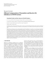
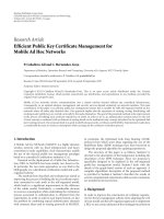
Figure 1: The result graphs for the tracker comparison experiments. The top row shows the distance error e
c
, the bottom row shows the
region error e
r
. The left-hand column contains the results for trackers without scale estimation, the right-hand column those with scale
estimation. The horizontal axis does not correspond to time, but to sorted aggregation over all test videos. In other words, each graph shows
“all” error quantiles (also known as percentiles). The vertical axis for e
c
has been truncated to 100 pixels to emphasize the relevant details.
4.2. Trust-region optimization
For the trust-region optimization, again the gradient and the
Hessian of the objective function have to be derived. As the
simplified objective function S
∗
(x) is a linear combination

of the simplified distance measures S
h
(x) for the individual
histograms h, the gradient of S
∗
(x)) is a linear combination
of the gradient in the single histogram case S
h
(x),
∂S
∗
(x)
∂x
i
=
∂
∂x
i


h∈H
β
h
S
h
(x)

=

h∈H

β
h
∂S
h
(x)
∂x
i
,
(21)
The same applies to the Hessian,
∂
2
S
∗
(x)
∂x
j
∂x
i
=
∂
∂x
j

∂S
∗
(x)
∂x
i


=
∂
∂x
j


h∈H
β
h
∂S
h
(x)
∂x
i

=

h∈H
β
h
∂
∂x
j

∂S
h
(x)
∂x
i


.
(22)
The factor ∂S
h
(x)/∂x
i
is the ith component of the gradient in
the single histogram case. The factor ∂/∂x
j
(∂S
h
(x)/∂x
i
) is the
entry (i, j) of the Hessian in the single histogram case. Details
can be found in [13].
6 EURASIP Journal on Image and Video Processing
0
20
40
60
80
e
c
00.20.40.60.8
Quantile
100
400
4000
(a)

0
20
40
60
80
e
c
00.20.40.60.8
Quantile
100
400
4000
(b)
0
0.2
0.4
0.6
0.8
1
e
r
00.20.40.60.8
Quantile
100
400
4000
(c)
0
0.2
0.4

0.6
0.8
1
e
r
00.20.40.60.8
Quantile
100
400
4000
(d)
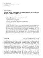
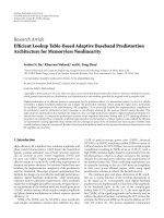
Figure 2: Same evaluation as in Figure 1 for three configurations of the CONDENSATION tracker with different numbers of particles.
Note that for the trust-region trackers, the simplifica-
tion of the objective function D
∗
to S
∗
is not necessary.
However, without the simplification, the gradient and the
Hessian of the objective function D
∗
(x)areno longer linear
combinations of the gradient and the Hessian for the full
single histogram distance measures D
h
and thus the resulting
expressions are more complicated and computationally more
expensive—without an obvious advantage. Note also, that
for the case of a common kernel for all features, the difference
between the single histogram and the multiple histogram

case is that the expression
w
t
(x, n) is replaced by w
t
(x, n),
which is the same expression as for the combined histogram
mean-shift tracker (see Sections 3.4 and 4.1).
5. ONLINE ADAPTATION OF FEATURE WEIGHTS
As described in Section 4, the feature weights β
h
, h ∈ H
are constant throughout the tracking process. However,
the most discriminative feature combination can vary over
time. For example, as the object moves, the surrounding
background can change drastically, or motion blur can have
a negative influence on edge features for a limited period of
time. Several authors have proposed online feature selection
mechanisms for tracking. They either select one feature [16]
or several features which they combine empirically after
performing tracking with each winning feature [17, 18].
A further approach computes an “artificial” feature using
F. Bajramovic et al. 7
principal component analysis [19]. Democratic integration
[20], on the other hand, assigns a weight to each feature
and adapts these weights based on the recent performance
of the individual features. Given our combined histogram
tracker (CHT), we follow the idea of dynamically adapting
the weight β
h

of each individual feature h. To emphasize this,
we use the notation β
h
(t) in this section. Unlike Democratic
Integration, we perform weight adaptation in an explicit and
very efficient tracking framework.
The central part of feature selection as well as adaptive
weighting is a measure for the tracking performance of each
feature. Typically, the discriminability between object and
surrounding background is estimated for each feature. In our
case, this quality measure is used to increase the weights of
good features and decrease the weights of bad features. In
the context of this work, a natural choice for such a quality
measure is the distance,
ρ
h
(t) = D
h

q
(h)

x(t)

, p
(h)

x(t)

, (23)

between the object histogram q
(h)
(x(t)) and the histogram
p
(h)
(x(t)) of an area surrounding the object ellipse. Both
histograms are extracted after tracking in frame t.Weapply
three different weight adaptation strategies.
(1) The weight of the feature h with the best quality ρ
h
(t)
is increased by multiplying with a factor γ (set to 1.3),
β
h
(t +1)= γβ
h
(t). (24)
Accordingly, the feature h

with the worst quality
ρ
h

(t) is decreased by dividing by γ,
β
h

(t +1)=
β
h


(t)
γ
. (25)
Upper and lower limits are imposed on β
h
for every
feature h to keep weights from diverging. We used the
bounds 0.01 and 100. This adaptation strategy is only
suited for two features (H
= 2).
(2) The weight β
h
(t +1)ofeachfeatureh is set to its
quality measure ρ
h
(t),
β
h
(t +1)= ρ
h
(t). (26)
(3) The weight β
h
(t+1) of each feature h is slowly adapted
toward ρ
h
(t) using a convex combination (IIR filter)
with parameter ν (set to 0.1 in our experiments),
β

h
(t +1)= νρ
h
(t)+(1−ν)β
h
(t). (27)
6. EXPERIMENTAL EVALUATION
6.1. Test set and evaluation criteria
In the experiments, we use some of the test videos of
the CAVIAR project [7], originally recorded for action and
behavior recognition experiments. The videos are perfectly
suited, since they are recorded in a “natural” environment,
with change in illumination and scale of the moving
0
0.2
0.4
0.6
0.8
e
r
0 t
1
400t
2
t
3
800
Frame
Hager
CONDENSATION

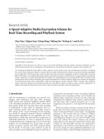
Figure 3: Comparison of the Hager and CONDENSATION
trackers using the e
r
error measure (28). The black rectangle shows
the ground truth. The white rectangle is from the Hager tracker,
the dashed rectangle from the CONDENSATION tracker. The
top, middle, and bottom images are from frames t
1
, t
2
,andt
3
,
respectively. The tracked person (almost) leaves the camera’s field
of view in the middle image, and returns shortly before time t
3
.The
Hager tracker is more accurate, but loses the person irretrievably,
while the CONDENSATION tracker is able to reacquire the person.
personsaswellaspartialocclusions.Mostimportantly,the
moving persons are hand-labelled, that is, for each frame, a
ground truth rectangle is stored. In case of the mean-shift
and trust-region trackers, the ground truth rectangles are
transformed into ellipses to avoid systematic errors in the
tracker evaluation based on (27).
In each experiment, a specific person was tracked. The
tracking system was given the frame number of the first
unoccluded appearance of the person, the accordant ground
truth rectangle around the person as initialization, and
the frame of the person’s disappearance. Aside from this

initialization, the trackers had no access to the ground truth
information. Twelve experiments were performed on seven
videos (some videos were reused, tracking a different person
each time).
To evaluate the results of the original trackers as well as
our extensions, we used an area-based criterion. We measure
the difference e
r
of the region A computed by the tracker and
the ground-truth region B,
e
r
(A, B):=
|
A \B|+ |B \ A|
|A| + |B|
= 1 −
|
A ∩B|
1/2

|A| + |B|

, (28)
where
|A| denotes the number of pixels in region A. This
error measure is zero if the two regions are identical, and
one if they do not overlap. If the two regions have the same
size, the error increases with increasing distance between the
8 EURASIP Journal on Image and Video Processing

0
0.2
0.4
0.6
0.8
1
e
r
00.20.40.60.8
Quantile
rgb
Edge
rgb-edge
fwa3-rgb-edge
Evaluation using all frames
(a)
0
0.2
0.4
0.6
0.8
1
e
r
00.20.40.60.8
Quantile
fwa1-rgb-edge
fwa2-rgb-edge
fwa3-rgb-edge
Evaluation using all frames

(b)
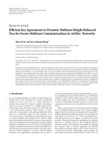
Figure 4:Sortederror(i.e.,allquantilesasinFigure 1) using CHT with RGB and gradient strength with constant weights (rgb-edge)and
three different feature weight adaptation mechanisms (fwa1-rgb-edge, fwa2-rgb-edge,andfwa3-rgb-edge), as well as single histogram trackers
using RGB (rgb) and edge histogram (edge). Results are given for the mean-shift tracker with scale estimation, Biweight-Kernel, and Kullback-
Leibler distance for all individual histograms.
center of both regions. Equal centers but different sizes are
also taken into account. We also compare the trackers using
the Euclidean distance e
c
between the centers of A and B.
6.2. General comparison
In the first part of the experiments, we give a general
comparison of the following six trackers, which were tested
withpuretranslationestimation,aswellaswithtranslation
and scale estimation.
(i) The region tracking algorithm of Hager and Bel-
humeur [2], working on a three-level Gaussian image
pyramid to enlarge the basin of convergence.
(ii) The hyperplane tracker, using a 150-point region and
initialized with 1000 training perturbation steps.
(iii) The mean-shift and two trust-region algorithms,
using an Epanechnikov weighting kernel, the Bhattacharyya
distance measure, and the HSV color histogram feature
introduced by P
´
erez et al. [6] for maximum comparability.
(iv) Finally, the CONDENSATION-based color his-
togram approach of P
´
erez et al. [6]. As this tracker is

computationally expensive, we choose only 400 particles
for the main comparison, and alternatively 100 and 4000.
Furthermore, we kept the particle size as low as possible:
two position parameters and an additional scale parameter
if applicable. The algorithm is thus restricted to a simplified
motion model, which estimates the velocity of the object by
taking the difference between the position estimates from
the last two frames. The predicted particles are diffused by a
zero-mean Gaussian distribution with a variance of 5 pixels
in each dimension.
These experiments were timed on a 2.8 GHz Intel Xeon
processor. The methods differ greatly in the time taken for
Table 1: Timing results for the first sequence, in milliseconds. For
each tracker, the time taken for initialization and the average time
per frame are shown with and without scale estimation.
Without scale With scale
Initial Per frame Initial Per frame
Hager 4 2.40 5 2.90
Hyperplane 557 2.22 548 2.21
Mean shift 2 1.04 2 2.75
Trust region 9 4.01 18 8.63
Trust region 1st 5 7.25 6 12.09
CONDENSATION 100 11 27.71 11 40.50
CONDENSATION 400 11 79.67 11 109.85
CONDENSATION 4000 14 706.62 14 962.02
initialization (once per sequence) and tracking (once per
frame). Ta b le 1 shows the results for the first sequence. Note
the long initialization of the hyperplane tracker due to train-
ing, and the long per-frame time of the CONDENSATION.
For each tracker, the errors e

c
and e
r
from all sequences
were concatenated and sorted. Figure 1 shows the measured
distance error e
c
and the region error e
r
for all trackers,
with and without scale estimation. Performance varies
widely between all tested trackers, showing strengths and
weaknesses of each individual method. There appears to be
no method which is universally “better” than the others.
The structure-based region trackers, Hager and hyper-
plane, are potentially very accurate, as can be seen at the left-
hand side of each graph, where they display a larger number
of frames with low errors. However, both are prone to losing
the target rather quickly, causing their errors to climb faster
F. Bajramovic et al. 9
than the other three methods. Particularly when scale is
also estimated, the additional degree of freedom typically
provides additional accuracy, but causes the estimation to
diverge sooner. This is due to strong appearance changes of
the tracked regions in these image sequences.
The CONDENSATION method, for the most part, is not
as accurate as the three local optimization methods: mean-
shift and the two trust-region variants. Figure 2 shows the
performance with three different numbers of particles, the
severe influence on computation times can be seen in Table 1 .

As expected, increasing the number of particles improves
the tracking results. However, the relative performance in
comparison with the other trackers is mostly unaffected.
We believe that this is partly due to the fact that time
constraints necessitate the use of a quickly computable
particle evaluation function, which does not include a spatial
kernel—in contrast to the other histogram-based methods.
Figure 3 shows a direct comparison between a locally
optimizing structural tracker (Hager) and the globally
optimizing histogram-based CONDENSATION tracker. It
is clearly visible that the Hager tracker provides more
accurate results, but cannot reacquire a lost target. The
CONDENSATION tracker, on the other hand, can continue
to track the person after it reappears.
The mean-shift and both trust-region trackers show
a very similar performance and provide the best overall
tracking if scale estimation is turned off. With scale estima-
tion, however, the mean-shift algorithm performs noticeably
better than the first-order trust-region approach, which
in turn is better than second-order trust-region tracker.
This is especially visible when comparing the region error
e
r
(Figure 1(d)), where the error in the scale component
plays an important role. This is probably caused by the
very different approaches to scale estimation in the two
types of trackers. While the trust-region trackers directly
incorporate scale estimation with variable aspect ratio into
the optimization problem, the mean-shift tracker uses a
heuristic approach which limits the maximum scale change

per frame (to 1% in our experiments [4, 13]). It seems
that this forcedly slow scale adaptation keeps the mean-shift
tracker from over adapting the scale to changes in object
and/or background appearance. The first-order trust-region
tracker seems to benefit from the fact that its first-order
optimization algorithm has worse convergence properties
than the second-order variant, which seems to reduce the
scale over adaption of the scale parameters.
Another very interesting aspect to note is that tracking
translation and scale, as opposed to tracking translation only,
does not generally improve the results of most trackers. The
two template trackers gain a little extra precision, but lose the
object much earlier. The changing appearance of the tracked
persons is a strong handicap for them as the image constancy
assumption is violated. The additional degree of freedom
opens up more chances to diverge toward local optima,
which causes the target to be lost sooner. The mean-shift
tracker does actually perform better with scale estimation.
The other histogram-based trackers are better in case of pure
translation estimation. They suffer from the fact that the
features themselves are typically rather invariant under scale
(a) (b)
Figure 5: Tracking results for one of the CAVIAR images sequences
(first and last image of the successfully tracked person). The
tracking results are almost identical to the ground truth regions
(ellipses).Notethescalechangeofthepersonbetweenthetwo
images.
changes. Once the scale is wrong, small translations of the
target can go completely unnoticed.
6.3. Improvements of the combined histogram tracker

In the second part of the experiments, we combined
two different histograms. The first is the standard color
histogram consisting of the RGB channels, abbreviated in
the figures as rgb. The second histogram is computed from
a Sobel edge strength image (edge), with the edge strength
normalized to fit the gray-value range from 0 to 255.
In Figure 4, the tracking accuracy of the mean-shift
tracker is shown. The graph displays the error e
r
accumulated
and sorted over all sequences (same scheme as in Figure 1).
In other words, the graph shows “all” error quantiles. The
reader can verify that a combination of RGB and gradient
strength histograms leads to an improvement of tracking
accuracy compared to a pure RGB histogram tracker, even
though the object is lost a bit earlier. We got similar results for
the corresponding trust-region tracker with our extension to
combined histograms. The weights β
h
for combining RGB
and edge histograms (compare (16)) have been empirically
set to 0.8and0.2. The computation time for one image is
on average approximately 2 milliseconds on a 3.4 GHz P4
compared to approximately 1 millisecond for a tracker using
one histogram only. A successful tracking example including
correct scale estimation is shown in Figure 5.
6.4. Improvements with weight adaptation
In the third part of the experiments, we evaluate the
performance of the CHT with weight adaptation. We include
the three feature weight adaptation mechanisms (fwa1, fwa2,

fwa3 according to the numbers in Section 5) in the experi-
ment of Section 6. All adaptation mechanisms are initialized
with both feature weights set to 0.5. Results are given in
Figure 4. The third weight adaptation mechanism (fwa3-rgb-
edge)performsalmostasgoodasthemanuallyoptimized
constant weights (rgb-edge). Figure 4(b) gives a comparison
of the three feature weight adaptation mechanisms. Here, the
third adaptation mechanism gives the best results.
As the RGB histogram dominates the gradient strength
histogram, we use the blue- and green color channels as
10 EURASIP Journal on Image and Video Processing
0
0.2
0.4
0.6
0.8
1
e
r
00.20.40.60.8
Quantile
Green
Blue
Green-blue
fwa1-green-blue
Evaluation using all frames
(a)
0
0.2
0.4

0.6
0.8
1
e
r
00.20.40.60.8
Quantile
fwa1-green-blue
fwa2-green-blue
fwa3-green-blue
Evaluation using all frames
(b)
Figure 6:Sortederror(i.e.,allquantilesasinFigure 1) using CHT with green and blue histograms with constant weights (green-blue)and
three different feature weight adaptation mechanisms (fwa1-green-blue, fwa2-green-blue, and fwa3-green-blue), as well as single histogram
trackers using a green (green) and a blue histogram (blue). Results are given for the mean-shift tracker with scale estimation, biweight-kernel,
and Kullback-Leibler distance for all individual histograms.
individual features in the second experiment. Both feature
weights are set to 0.5 for the CHT with and without weight
adaptation. All other parameters are kept as in the previous
experiment. The results are displayed in Figure 6. The single
histogram tracker using the green feature performs better
than the blue feature. The CHT gives similar results to the
blue feature, which is caused by bad feature weights. With
weight adaptation, the performance of the CHT is greatly
improved and almost reaches that of the green feature.
This shows that, even though the single histogram tracker
with the green feature gives the best results, the CHT with
weight adaptation performs almost equally well without a
good initial guess for the best single feature or the best
constant feature weights. Figure 6(b) gives a comparison

of the three feature weight adaptation mechanisms. Here,
the first adaptation mechanism gives the best results. The
average computation time for one image is approximately 4
milliseconds on a 3.4 GHz P4 compared to approximately 2
milliseconds for the CHT with constant weights.
7. CONCLUSIONS
As the first contribution of this paper, we presented a
comparative evaluation of five state-of-the-art algorithms
for data-driven object tracking, namely Hager’s region
tracking technique [2],Jurie’shyperplaneapproach[3], the
probabilistic color histogram tracker of P
´
erez et al. [6],
Comaniciu’s mean-shift tracking approach [4], and the trust-
region method introduced by Liu and Chen [5]. All of
those trackers have the ability to estimate the position and
scale of an object in an image sequence in real-time. The
comparison was carried out on part of the CAVIAR video
database, which includes ground-truth data. The results of
our experiments show that, in cases of strong appearance
change, the template-based methods tend to lose the object
sooner than the histogram-based methods. On the other
hand, if the appearance change is minor, the template-based
methods surpass the other approaches in tracking accuracy.
Comparing the histogram-based methods among each other,
the mean-shift approach [4] leads to the best results. The
experiments also show that the probabilistic color histogram
tracker [6] is not quite as accurate as the other techniques,
but is more robust in case of occlusions and appearance
changes. Note, however, that the accuracy of this tracker

depends on the number of particles, which has to be chosen
rather small to achieve real-time precessing.
As the second contribution of our paper, we presented
a mathematically consistent extension of histogram-based
tracking, which we call combined histogram tracker (CHT).
We showed that the corresponding optimization problems
can still be solved using the mean-shift as well as the trust-
region algorithms without loosing real-time capability. The
formulation allows for the combination of an arbitrary
number of histograms with different dimensions and sizes,
as well as individual distance functions for each feature. This
allows for high flexibility in the application of the method.
In the experiments, we showed that a combination of
two features can improve tracking results. The improvement
of course depends on the chosen histograms, the weights,
and the object to be tracked. We would like to stress again
that similar results were achieved using the trust-region
algorithm, although the presentation in this paper was
focused on the mean-shift algorithm. For more details, the
reader is referred to [13]. We also presented three online
weight adaptation mechanisms for the combined histogram
tracker. The benefit of feature weight adaptation is that an
F. Bajramovic et al. 11
initial choice of a single best feature or optimal combination
weights is no longer necessary, as has been shown in the
experiments. One important result is that the CHT with (and
also without) weight adaptation can still be applied in real-
time on standard PC hardware.
In our future work, we will evaluate the performance
of the weight adaptation mechanisms on more than two

features and investigate more sophisticated adaptation mech-
anisms. We are also going to systematically compare the CHT
with the other trackers described in this paper.
ACKNOWLEDGMENTS
This work was partially funded by the German Science
Foundation (DFG ) under grant SFB 603/TP B2. This work
was partially funded by the European Commission 5th IST
Programme—Project VAMPIRE.
REFERENCES
[1] B. Deutsch, Ch. Gr
¨
aßl, F. Bajramovic, and J. Denzler, “A
comparative evaluation of template and histogram based 2D
tracking algorithms,” in Proceedings of the 27th Annual Meeting
of the German Association for Pattern Recognition (DAGM ’05),
pp. 269–276, Vienna, Austria, August-September 2005.
[2] G.D.HagerandP.N.Belhumeur,“Efficient region tracking
with parametric models of geometry and illumination,” IEEE
Transactions on Pattern Analysis and Machine Intelligence, vol.
20, no. 10, pp. 1025–1039, 1998.
[3] F. Jurie and M. Dhome, “Hyperplane approach for template
matching,” IEEE Transactions on Pattern Analysis and Machine
Intelligence, vol. 24, no. 7, pp. 996–1000, 2002.
[4] D. Comaniciu, V. Ramesh, and P. Meer, “Kernel-based object
tracking,” IEEE Transactions on Pattern Analysis and Machine
Intelligence, vol. 25, no. 5, pp. 564–577, 2003.
[5] T L. Liu and H T. Chen, “Real-time tracking using trust-
region methods,” IEEE Transactions on Pattern Analysis and
Machine Intelligence, vol. 26, no. 3, pp. 397–402, 2004.
[6] P. P

´
erez, C. Hue, J. Vermaak, and M. Gangnet, “Color-based
probabilistic tracking,” in Proceedings of the 7th European
Conference on Computer Vision (ECCV ’02), vol. 1, pp. 661–
667, Copenhagen, Denmark, May 2002.
[7] CAVIAR, EU funded project, IST 2001 37540, 2004,
/>[8] F.Bajramovic,Ch.Gr
¨
aßl, and J. Denzler, “Efficient combina-
tion of histograms for real-time tracking using mean-shift and
trust-region optimization,” in Proceedings of the 27th Annual
Meeting of the German Association for Pattern Recognition
(DAGM ’05), pp. 254–261, Vienna, Austria, August-September
2005.
[9] Cheng, “Mean shift, mode seeking, and clustering,” IEEE
Transactions on Pattern Analysis and Machine Intelligence, vol.
17, no. 8, pp. 790–799, 1995.
[10] A. R. Conn, N. I. M. Gould, and P. L. Toint, Trust-Region
Methods, SIAM, Philadelphia, Pa, USA, 2000.
[11] S. Baker, R. Gross, and I. Matthews, “Lucas-Kanade 20 years
on: a unifying framework: part 4,” Tech. Rep. CMU-RI-TR-04-
14, Robotics Institute, Carnegie Mellon University, Pittsburgh,
Pa, USA, 2004.
[12] M. P. Wand and M. C. Jones, Kernel Smoothing, Chapman &
Hall/CRC, Boca Raton, Fla, USA, 1995.
[13] F. Bajramovic, Kernel-basierte Objektverfolgung, M.S. thesis,
Computer Vision Group, Department of Mathematics and
Computer Science, University of Passau, Lower Bavaria,
Germany, 2004.
[14] M. Isard and A. Blake, “CONDENSATION—conditional

density propagation for visual tracking,” International Journal
of Computer Vision, vol. 29, no. 1, pp. 5–28, 1998.
[15] D. Comaniciu and P. Meer, “Mean shift: a robust approach
toward feature space analysis,” IEEE Transactions on Pattern
Analysis and Machine Intelligence, vol. 24, no. 5, pp. 603–619,
2002.
[16] H. Stern and B. Efros, “Adaptive color space switching
for tracking under varying illumination,” Image and Vision
Computing, vol. 23, no. 3, pp. 353–364, 2005.
[17] R. T. Collins, Y. Liu, and M. Leordeanu, “Online selection of
discriminative tracking features,” IEEE Transactions on Pattern
Analysis and Machine Intelligence, vol. 27, no. 10, pp. 1631–
1643, 2005.
[18] B. Kwolek, “Object tracking using discriminative feature
selection,” in Proceedings of the 8th International Conference on
Advanced Concepts for Intelligent Vision Systems (ACIVS’06)
,
pp. 287–298, Antwerp, Belgium, September 2006.
[19] B. Han and L. Davis, “Object tracking by adaptive feature
extraction,” in Proceedings of the International Conference on
Image Processing (ICIP ’04), vol. 3, pp. 1501–1504, Singapore,
October 2004.
[20] J. Triesch and C. von der Malsburg, “Democratic integration:
self-organized integration of adaptive cues,” Neural Computa-
tion, vol. 13, no. 9, pp. 2049–2074, 2001.