Báo cáo hóa học: "Research Article About Advances in Tensor Data Denoising Methods" doc

Hindawi Publishing Corporation
EURASIP Journal on Advances in Signal Processing
Volume 2008, Article ID 235357, 12 pages
doi:10.1155/2008/235357
Research Article
About Advances in Tensor Data Denoising Methods
Julien Marot, Caroline Fossati, and Salah Bourennane
Institut Fresnel CNRS UMR 6133, Ecole Centrale Marseille, Universit
´
ePaulC
´
ezanne, D.U. de Saint J
´
er
ˆ
ome,
13397 Marseille Cedex 20, France
Correspondence should be addressed to Salah Bourennane,
Received 15 December 2007; Revised 15 June 2008; Accepted 31 July 2008
Recommended by Lisimachos P. Kondi
Tensor methods are of great interest since the development of multicomponent sensors. The acquired multicomponent data
are represented by tensors, that is, multiway arrays. This paper presents advances on filtering methods to improve tensor data
denoising. Channel-by-channel and multiway methods are presented. The first multiway method is based on the lower-rank
(K
1
, , K
N
) truncation of the HOSVD. The second one consists of an extension of Wiener filtering to data tensors. When multiway
tensor filtering is performed, the processed tensor is flattened along each mode successively, and singular value decomposition of
the flattened matrix is performed. Data projection on the singular vectors associated with dominant singular values results in noise
reduction. We propose a synthesis of crucial issues which were recently solved, that is, the estimation of the number of dominant

singular vectors, the optimal choice of flattening directions, and the reduction of the computational load of multiway tensor
filtering methods. The presented methods are compared through an application to a color image and a seismic signal, multiway
Wiener filtering providing the best denoising results. We apply multiway Wiener filtering and its fast version to a hyperspectral
image. The fast multiway filtering method is 29 times faster and yields very close denoising results.
Copyright © 2008 Julien Marot et al. This is an open access article distributed under the Creative Commons Attribution License,
which permits unrestricted use, distribution, and reproduction in any medium, provided the original work is properly cited.
1. INTRODUCTION
Tensor data modelling and tensor analysis have been
improved and used in several application fields. These appli-
cation fields are quantum physics, economy, psychology,
data analysis, chemometrics [1]. Specific applications are
the characterization of DS-CDMA systems [2], and the
classification of facial expressions. For this application, a
multilinear independent component analysis [3]wascreated.
Another specific application is in particular the processing
and visualization of medical images obtained through mag-
netic resonance imaging [4].
Tensor data generalize the classical vector and matrix
data to entities with more than two dimensions [1, 5, 6].
In signal processing, there was a recent development of
multicomponent sensors, especially in imagery (color or
multispectral images, video, etc.) and seismic fields (an
antenna of sensors selects and records signals of a given
polarization). The digital data obtained from these sensors
are fundamentally multiway arrays, which are called, in
the signal processing community and in this paper in
particular, higher-order tensor objects, or tensors. Each
multiway array entry corresponds to any quantity. The
elements of a multiway array are accessed via several indexes.
Each index is associated with a dimension of the tensor

generally called “nth-mode” [5, 7–10]. Measured data are
not fully reliable since any real sensor will provide noisy
and possibly incomplete and degraded data. Therefore, all
problems dealt with in conventional signal processing such as
filtering, restoration from noisy data must also be addressed
when dealing with tensor signals [6, 11].
In order to keep the data tensor as a whole entity,
new signal processing methods have been proposed [12–
15]. Hence, instead of adapting the data tensor to the
classical matrix-based algebraic techniques [16, 17](by
rearrangement or splitting), these new methods propose
to adapt their processing to the tensor structure of the
multicomponent data. Multilinear algebra is adapted to
multicomponent data. In particular, it involves two tensor
decomposition models. They generalize that the matrix SVD
has been initially developed in order to achieve a multimode
principal component analysis and recently used in tensor
signal processing. They rely on two models: PARAFAC and
TUCKER3 models.
(1) The PARAFAC model and the CANDECOMP model
developed in [18, 19], respectively. In [20], the link was
2 EURASIP Journal on Advances in Signal Processing
set between CANDECOMP and PARAFAC models. The
CANDECOMP/PARAFAC model, referred to as the CP
model [21], has recently been applied to food indus-
try [22], array processing [23], and telecommunications
[2]. PARAFAC decomposition of a tensor containing data
received on an array of sensors yields strong identifiability
results. Identifiability results depend firstly on a relationship
between the rank, in the sense of PARAFAC decomposi-

tion, of the data tensor, secondly on the Kruskal rank of
matrices which characterize the propagation and source
amplitude.
In particular, nonnegative tensor factorization [24]is
used in multiway blind source separation, multidimensional
data analysis, and sparse signal/image representations. Fixed
point optimization algorithm proposed in [25]andmore
specifically fixed-point alternating least squares [25]canbe
used to achieve such a decomposition.
(2) The TUCKER3 model [10, 26] adopted in higher-
order SVD (HOSVD) [7, 27] and in LRTA-(K
1
, , K
N
)
(lower-rank (K
1
, , K
N
) tensor approximation) [8, 28,
29]. We denote by HOSVD-(K
1
, , K
N
) the truncation
of HOSVD, performed with ranks (K
1
, , K
N
), in modes

1, , N, respectively. This model has recently been used
as multimode PCA in seismics for wave separation based
on a subspace method, in image processing for face
recognition and expression analysis [30, 31]. Indeed tensor
representation improves automatic face recognition in an
adapted independent component analysis framework. “Mul-
tilinear independent component analysis” [30] distinguishes
between different factors, or modes, inherent to image
formation. In particular, this was used for classification of
facial expressions. The TUCKER3 model is also used for
noise filtering of color images [14].
Each decomposition method corresponds to one defini-
tion of the tensor rank. PARAFAC decomposes a tensor into
a summation of rank one tensors. The HOSVD-(K
1
, , K
N
)
and the LRTA-(K
1
, , K
N
) rely on the nth-mode rank
definition, that is, the matrix rank of the tensor nth-mode
flattening matrix [7, 8]. Both methods perform data projec-
tion onto a lower-rank subspace. In this paper, we focus on
data denoising [6, 11] by HOSVD-(K
1
, , K
N

), lower-rank
(K
1
, , K
N
) approximation, and multiway Wiener filtering
[6]. Lower-rank (K
1
, , K
N
) approximation and multiway
Wiener filtering were further improved in the past two years.
Some crucial issues were recently solved to improve tensor
data denoising. Statistical criteria were adapted to estimate
the values of signal subspace ranks [32]. A particular choice
of flattening directions improves the results in terms of signal
to noise ratio [33, 34]. Multiway filtering algorithms rely on
alternating least squares (ALS) loops, which include several
costly SVD. We propose to replace SVD by the faster fixed
point algorithm proposed in [35]. This paper is a synthesis
of the advances that solve these issues. The motivation is
that by collecting papers from a range of application areas
(including hyperspectral imaging and seismics), the field of
tensor signal denoising can be more clearly presented to the
interested scientific community, and the field itself may be
cross-fertilized with concepts coming from statistics or array
processing.
Section 2 presents the tensor model and its main prop-
erties. Section 3 states the tensor filtering issue. Section 4
presents classical channel-by-channel filtering methods.

Section 5 reminds the principles of two multiway tensor
filtering methods, namely lower-rank tensor approximation
(LRTA) and multiway Wiener filtering (MWF), developed
over the past few years. Section 6 presents all recently pro-
posed improvements for multiway tensor filtering methods
which permit an adequate choice of several parameters
for multiway filtering methods. The parameter choice is
performed as follows: the signal subspace ranks are estimated
by a statistical criteria, nonorthogonal tensor flattening
for the improvement of tensor data denoising when main
directions are present, and fast versions of LRTA and MWF
obtained by adapting fixed point and inverse power algo-
rithms for the estimation of leading eigenvectors and smallest
eigenvalue. Section 7 exemplifies the presented algorithms by
an application to color image and seismic signal denoising;
we study the computational load of LRTA and MWF and
their fast version by an application to hyperspectral images.
2. DATA TENSOR PROPERTIES
We define a tensor of order N as a multidimensional array
whoseentriesareaccessedviaN indexes. A tensor is denoted
by A
∈ C
I
1
×···×I
N
, where each element is denoted by a
i
1
···i

N
,
and
C is the complex manifold. An order N tensor has size
I
n
in mode n,wheren refers to the nth index. In signal
processing, tensors are built on vector spaces associated with
quantities such as length, width, height, time, color channel,
and so forth. Each mode of the tensor is associated with
one quantity. For example, seismic signals can be modelled
by complex valued third-order tensors. Tensor elements
can be complex values, to take into account the phase
shifts between sensors [6]. The three modes are associated,
respectively, with sensor, time, and polarization. In image
processing, multicomponent images can be modelled as
third-order tensors: two dimensions for rows and columns,
and one dimension for the spectral channel. In the same
way, a sequence of color images can be modelled by a
fourth-order tensor by adding to the previous model one
mode associated with the time sampling. Let us define E
(n)
as the nth-mode vector space of dimension I
n
, associated
with the nth-mode of tensor A. By definition, E
(n)
is
generated by the column vectors of the nth-mode flattening
matrix. The nth-mode flattening matrix A

n
of tensor A ∈
R
I
1
×···×I
N
is defined as a matrix from R
I
n
×M
n
,whereM
n
=
I
n+1
I
n+2
···I
N
I
1
I
2
···I
n−1
. For example, when we consider
a third-order tensor, the definition of the matrix flattening
involves the dimensions I

1
, I
2
, I
3
in a backward cyclic way
[7, 21, 36]. When dealing with a 1st-mode flattening of
dimensionality I
1
× (I
2
I
3
), we formally assume that the index
i
2
values vary more slowly than index i
3
values. For all n = 1
to 3, A
n
columns are the I
n
-dimensional vectors obtained
from A by varying the index i
n
from 1 to I
n
and keeping the
other indexes fixed. These vectors are called the nth-mode

vectors of tensor A. In the following, we use the operator
“
×
n
” as the “nth-mode product” that generalizes the matrix
product to tensors. Given A
∈ R
I
1
×···×I
N
and a matrix
Julien Marot et al. 3
U ∈ R
J
n
×I
n
, the nth-mode product between tensor A and
matrix U leads to the tensor B
= A×
n
U, which is a tensor of
R
I
1
×···I
n−1
×J
n

×I
n+1
×···×I
N
, whose entries are
b
i
1
···i
n−1
j
n
i
n+1
···i
N
=
I
n

i
n
=1
a
i
1
···i
n−1
i
n

i
n+1
···i
N
u
j
n
i
n
. (1)
Next section presents the principles of subspace-based tensor
filtering methods.
3. TENSOR FILTERING PROBLEM FORMULATION
The tensor data extend the classical vector data. The
measurement of a multiway signal X by multicomponent
sensors with additive noise N results in a data tensor R such
that
R
= X + N . (2)
R, X,andN are tensors of order N from
R
I
1
×···×I
N
.Tensors
N and X represent noise and signal parts of the data,
respectively. The goal of this study is to estimate the expected
signal X thanks to a multidimensional filtering of the data
[6, 11, 13, 14]:


X = R×
1
H
(1)
×
2
H
(2)
×
3
···×
N
H
(N)
,(3)
Equation (3)performsnth-mode filtering of data tensor R
by nth-mode filter H
(n)
.
In this paper, we assume that the noise N is independent
from the signal X, and that the nth-mode rank K
n
is smaller
than the nth-mode dimension I
n
(K
n
<I
n

, ∀n = 1toN).
Then, it is possible to extend the classical subspace approach
to tensors by assuming that, whatever the nth-mode, the
vector space E
(n)
is the direct sum of two orthogonal
subspaces, namely, E
(n)
1
and E
(n)
2
,definedas
(i) E
(n)
1
is the subspace of dimension K
n
, spanned by the
K
n
singular vectors and associated with the K
n
largest
singular values of matrix X
n
; E
(n)
1
is called the signal

subspace [37–40];
(ii) E
(n)
2
is the subspace of dimension I
n
− K
n
, spanned by
the I
n
− K
n
singular vectors and associated with the
I
n
− K
n
smallest singular values of matrix X
n
; E
(n)
2
is
called the noise subspace [37–40].
Hence, one way to estimate signal tensor X from noisy
data tensor R is to estimate E
(n)
1
in every nth-mode of R.

The following section presents tensor channel-by-channel
filtering methods based on nth-mode signal subspaces.
We present further a method to estimate the dimensions
K
1
, K
2
, , K
N
.
4. CHANNEL-BY-CHANNEL FILTERING
The classical algebraic methods operate on two-dimensional
data matrices and are based on the singular value decom-
position (SVD) [37, 41, 42], and on Eckart-Young theorem
concerning the best lower-rank approximation of a matrix
[16] in the least-squares sense. Channel-by-channel filtering
consists first of splitting data tensor R, representing the
noisy multicomponent image into two-dimensional “slice
matrices” of data, each representing a specific channel.
According to the classical signal subspace methods [43], the
left and right signal subspaces, corresponding to, respectively,
the column and the row vectors of each slice matrix, are
simultaneously determined by processing the SVD of the
matrix associated with the data of the slice matrix. Let
us consider the slice matrix R(:, :, i
3
, , i
j
, , i
N

)ofdata
tensor R.ProjectorsP on the left signal subspace and Q on
the right signal subspace are built from, respectively, the left
and the right singular vectors associated with the K largest
singular values of R(:, :, i
3
, , i
j
, , i
N
). The parameter K
simultaneously defines the dimensions of the left and right
signal subspaces. Applying the projectors P and Q on the
slice matrix R(:, :, i
3
, , i
j
, , i
N
) amounts to compute its
best lower-rank K matrix approximation [16] in the least-
squares sense. The filtering of each slice matrix of data tensor
R separately is called in the following “channel-by-channel”
SVD-based filtering of R.Itisdetailedin[5].
Channel-by-channel SVD-based filtering is appropriate
only on some conditions. For example, applying SVD-based
filtering to an image is generally appropriate when the rows
or columns of an image are redundant, that is, linearly
dependent. In this case, the rank K oftheimageisequal
to the number of linearly independent rows or columns.

It is only in this case that it would be safe to throw out
eigenvectors from K +1on.
Other channel-by-channel processings are the following:
consecutive Wiener filtering of each channel (2D-Wiener),
PCA followed by 2D-Wiener (PCA-2D Wiener), or soft
wavelet threshold (SWT). PCA aims at decorrelating the data
(PCA-2D SWT)[44–46].
Channel-by-channel filtering methods exhibit a major
drawback; they do not take into account the relationships
between the components of the processed tensor. Next
section presents multiway filtering methods that process
jointly all data ways.
5. REVIEW OF MULTIWAY FILTERING METHODS
Multiway filtering methods process jointly all slice matrices
of a tensor, which improves the denoising results compared
to channel-by-channel processings [6, 11, 13, 14, 32].
5.1. Lower-rank tensor approximation
The LRTA-(K
1
, , K
N
)ofR minimizes the tensor Frobenius
norm (square root of the summation of squared modulus
of all terms)
R − B subject to the condition that B ∈
R
I
1
×···×I
N

is a rank-(K
1
, , K
N
)tensor.Thedescription
of TUCKALS3 algorithm, used in lower-rank (K
1
, , K
N
)
approximation is provided in Algorithm 1.
According to step 3(a)i, B
(n),k
represents data tensor R
filtered in every mth-mode but the nth-mode, by projection-
filters P
(m)
l
,withm
/
= n, l = k if m>nand l = k +1ifm<
n. TUCKALS3 algorithm has recently been used to process
4 EURASIP Journal on Advances in Signal Processing
(1) Input: data tensor R and dimensions K
1
, , K
N
of all nth-mode signal subspaces.
(2) Initialization k
= 0: for n = 1toN, calculate the projectors P

(n)
0
given by HOSVD-(K
1
, , K
N
):
(a) nth-mode flatten R into matrix R
n
,
(b) compute the SVD of R
n
,
(c) compute matrix U
(n)
0
formed by the K
n
eigenvectors associated with the K
n
largest singular values of R
n
.
U
(n)
0
is the initial matrix of the nth-mode signal subspace orthogonal basis vectors,
(d) form the initial orthogonal projector P
(n)
0

= U
(n)
0
U
(n)
T
0
on the nth-mode signal subspace,
(e) compute the truncation of HOSVD, with signal subspace ranks (K
1
, , K
N
), of tensor R given by
B
0
= R×
1
P
(1)
0
×
2
···×
N
P
(N)
0
.
(3) ALS loop
Repeat until convergence, that is, for example, while

B
k+1
− B
k

2
>ε, ε>0, being a prior fixed threshold,
(a) for n
= 1toN,
(i) form B
(n),k
:
B
(n),k
= R×
1
P
(1)
k+1
×
2
···×
n−1
P
(n−1)
k+1
×
n+1
P
(n+1)

k
×
n+2
···×
N
P
(N)
k
,
(ii) nth-mode flatten tensor B
(n),k
into matrix B
(n),k
n
,
(iii) compute matrix C
(n),k
= B
(n),k
n
R
T
n
,
(iv) compute matrix U
(n)
k+1
composed of the K
n
eigenvectors associated with the K

n
largest eigenvalues of C
(n),k
.
U
(n)
k
is the matrix of the nth-mode signal subspace orthogonal basis vectors at the kth iteration,
(v) compute P
(n)
k+1
= U
(n)
k+1
U
(n)
T
k+1
,
(b) compute B
k+1
= R×
1
P
(1)
k+1
×
2
···×
N

P
(N)
k+1
,
(c) increment k.
(4) Output
The estimated signal tensor is obtained through

X = R×
1
P
(1)
k
stop
×
2
···×
N
P
(N)
k
stop
.

X is the lower-rank (K
1
, , K
N
)
approximation o R,wherek

stop
is the index of the last iteration after the convergence of TUCKALS3 algorithm.
Algorithm 1: Lower-rank (K
1
, , K
N
) approximation—TUCKALS3 algorithm.
a multimode PCA in order to perform white noise removal
in color images, and denoising of multicomponent seismic
waves [11, 14].
5.2. Multiway wiener filtering
Let R
n
, X
n
,andN
n
be the nth-mode flattening matrices
of tensors R, X,andN , respectively. In the previous
subsection, the estimation of signal tensor X has been
performed by projecting noisy data tensor R on each nth-
mode signal subspace. The nth-mode projectors have been
estimated thanks to multimode PCA achieved by lower-
rank (K
1
, , K
N
) approximation. In spite of the good results
provided by this method, it is possible to improve the tensor
filtering quality by determining nth-mode filters H

(n)
, n = 1
to N,in(3), which optimize an estimation criterion. The
most classical method is to minimize the mean square error
between the expected signal tensor X and the estimated
signal tensor

X given in (3):
e

H
(1)
, , H
(N)

=
E



X − R×
1
H
(1)
×
2
···×
N
H
(N)



2

.
(4)
Due to the criterion which is minimized, filters H
(n)
, n = 1
to N,canbecalled“nth-mode Wiener filters” [6].
According to the calculations presented in [6], the
minimization of (4)withrespecttofilterH
(n)
,forfixed
H
(m)
, m
/
= n, leads to the following expression of nth-mode
Wiener filter [6]:
H
(n)
= γ
(n)
XR
Γ
(n)
RR
−1
. (5)

The expressions of γ
(n)
XR
and Γ
(n)
RR
can be found in [6]. γ
(n)
XR
depends on data tensor R and on signal tensor X. Γ
(n)
RR
only
depends on data tensor R.
In order to obtain H
(n)
through (5), we suppose that the
filters
{H
(m)
, m = 1toN, m
/
= n} are known. Data tensor
R is available, but signal tensor X is unknown. So, only
the term Γ
(n)
RR
can be derived, and not the term γ
(n)
XR

.Hence,
some more assumptions on X have to be made in order
to overcome the indetermination over γ
(n)
XR
[6, 13]. In the
one-dimensional case, a classical assumption is to consider
that a signal vector is a weighted combination of the signal
subspace basis vectors. In extension to the tensor case, [6, 13]
have proposed to consider that the nth-mode flattening
matrix X
n
can be expressed as a weighted combination of K
n
vectors from the nth-mode signal subspace E
(n)
1
:
X
n
= V
(n)
s
O
(n)
,(6)
with X
n
∈ R
I

n
×M
n
,andV
(n)
s
∈ R
I
n
×K
n
being the matrix
containing the K
n
orthonormal basis vectors of nth-mode
signal subspace E
(n)
1
.MatrixO
(n)
∈ R
K
n
×M
n
is a weight matrix
and contains the whole information on expected signal
tensor X. This model implies that signal nth-mode flattening
matrix X
n

is orthogonal to nth-mode noise flattening matrix
Julien Marot et al. 5
N
n
, since signal subspace E
(n)
1
and noise subspace E
(n)
2
are
supposed mutually orthogonal. Supposing that noise N in
(2) is white, Gaussian, and independent from signal X,and
introducing the signal model equation (6)in(5)leadstoa
computable expression of nth-mode Wiener filter H
(n)
(see
[6]):
H
(n)
= V
(n)
s
γ
(n)
OO
Λ
(n)
−1
Γs

V
(n)
T
s
. (7)
We d efi ne m at ri x T
(n)
as
T
(n)
= H
(1)
⊗···⊗H
(n−1)
⊗ H
(n+1)
⊗···⊗H
(N)
,(8)
where
⊗ stands for Kronecker product, and matrix Q
(n)
as
Q
(n)
= T
(n)
T
T
(n)

. (9)
In (7), γ
(n)
OO
Λ
(n)
−1
Γs
is a diagonal weight matrix given by
γ
(n)
OO
Λ
(n)
−1
Γs
= diag

β
1
λ
Γ
1
, ,
β
K
n
λ
Γ
K

n

, (10)
where λ
Γ
1
, , λ
Γ
K
n
are the K
n
largest eigenvalues of Q
(n)
-
weighted covariance matrix Γ
(n)
RR
= E[R
n
Q
(n)
R
T
n
]. Parameters
β
1
, , β
K

n
depend on λ
γ
1
, , λ
γ
K
n
which are the K
n
largest
eigenvalues of T
(n)
-weighted covariance matrix
γ
(n)
RR
= E[R
n
T
(n)
R
T
n
], according to the following relation:
β
k
n
= λ
γ

k
n
− σ
(n)
2
Γ
, ∀k
n
= 1, , K
n
. (11)
Superscript γ refers to the T
(n)
-weighted covariance, and
subscript Γ to the Q
(n)
-weighted covariance. σ
(n)
2
Γ
is the
degenerated eigenvalue of noise T
(n)
-weighted covariance
matrix γ
(n)
NN
= E[N
n
T

(n)
N
T
n
]. Thanks to the additive noise and
the signal independence assumptions, the I
n
− K
n
smallest
eigenvalues of γ
(n)
RR
are equal to σ
(n)
2
Γ
,andthus,canbe
estimated by the following relation:
σ
(n)
2
Γ
=
1
I
n
− K
n
I

n

k
n
=K
n
+1
λ
γ
k
n
. (12)
In order to determine the nth-mode Wiener filters
H
(n)
that minimizes the mean square error (see (4)), the
alternating least squares (ALSs) algorithm has been proposed
in [6, 13]. It can be summarized in Algorithm 2.
Both lower-rank tensor approximation and multiway
tensor filtering methods are based on singular value decom-
position. We propose to adapt faster methods to estimate
only the needed leading eigenvectors and dominant eigen-
values.
6. CHOICE OF PARAMETERS FOR MULTIWAY
FILTERING METHODS
6.1. nth-mode signal subspace rank estimation by
statistical criteria
The subspace-based tensor methods project the data onto
a lower-dimensional subspace of each nth-mode. For the
LRTA-(K

1
, K
2
, , K
N
), the (K
1
, K
2
, , K
N
)-parameter is the
number of eigenvalues of the flattened R
n
(for n = 1
to N) which permits an optimal approximation of R in
the least squares sense. For the multiway Wiener filter, it
is the number of eigenvalues which permits an optimal
restoration of X in the least mean squares sense. In a
noisy environment, it is equivalent to the useful nth-mode
signal subspace dimension. Moreover, because the eigenvalue
distribution of the nth-mode flattened matrix R
n
depends
on the noise power of N , the K
n
-value decreases when noise
power increases.
Finding the correct K
n

-values which yield an optimum
restoration appears, for two reasons, as a good strategy to
improve the denoising results [32]. Actually, for all nth-
modes, if K
n
is too small, some information is lost after
restoration, and if K
n
is too large, some noise may be
included in the restored information. Because the num-
ber of feasible (K
1
, K
2
, , K
N
) combinations is equal to
I
1
·I
2
·····I
N
which may be large, an estimation method
is chosen rather than empirical method. We review a
method, for the K
n
-value estimation for each nth-mode,
which adapts the well-know minimum description length
(MDL) detection criterion [47]. The optimal signal subspace

dimension is obtained by minimizing MDL criterion. The
useful signal subspace dimension is equal to the lower nth-
mode rank of the nth-mode flattened matrix R
n
.
Consequently, for each mode, the MDL criterion can be
expressed as
MDL(k)
=−log


i=I
n
i=k+1
λ
1/(I
n
−k)
i
(1/(I
n
− k))

i=I
n
i=k+1
λ
i

(I

n
−k)M
n
+
1
2
k(2I
n
− k)log M
n
.
(13)
When we consider lower-rank tensor approximation,
(λ
i
)
1≤i≤I
n
are either the I
n
singular values of R
n
(see step
2c of Algorithm 1), or the the I
n
eigenvalues of C
(n),k
(see
step (3)(a)iv). When we consider multiway Wiener filtering,
(λ

i
)
1≤i≤I
n
are the I
n
eigenvalues of either matrix γ
(n)
RR
or matrix
Γ
(n)
RR
(see steps 2(a)iiB and 2(a)iiE).
The nth-mode rank K
n
is the value of k (k ∈ [1, , I
n
−
1]) which minimizes MDL criterion.
The estimation of the signal subspace dimension of each
mode is performed at each ALS iteration.
6.2. Flattening directions for SNR improvement
To improve denoising quality, flattening is performed along
main directions in the image, which are estimated by SLIDE
algorithm [48].
6.2.1. Rank reduction and flattening directions
Let us consider a matrix A of size I
1
×I

1
which could represent
an image containing a straight line. The rank of this matrix
is closely linked to the orientation of the line: an image with
a horizontal or a vertical line has rank 1, else it is more
than one. The limit case is when the straight line is along
6 EURASIP Journal on Advances in Signal Processing
(1) Initialization k = 0: R
0
= R ⇔ H
(n)
0
= I
In
, identity matrix, for all n = 1toN.
(2) ALS loop:
repeat until convergence, that is,
R
k+1
− R
k

2
<ε, with ε>0 a prior fixed threshold,
(a) for n
= 1toN,
(i) form R
(n),k
:
R

(n),k
= R×
1
H
(1)
k+1
×
2
···×
n−1
H
(n−1)
k+1
×
n+1
H
(n+1)
k
×
n+2
×
N
H
(N)
k
,
(ii) determine H
(n)
k+1
= arg min

Z
(n)
X − R
(n),k
×
n
Z
(n)

2
subject to Z
(n)
∈ R
I
n
×I
n
thanks to the following procedure:
(A) nth-mode flatten R
(n),k
into R
(n),k
n
= R
n
(H
(1)
k+1
⊗···⊗H
(n−1)

k+1
⊗ H
(n+1)
k
⊗···⊗H
(N)
k
)
T
,andR into R
n
,
(B) compute γ
(n)
RR
= E[R
n
R
(n),k
n
T
],
(C) determine λ
γ
1
, , λ
γ
K
n
,theK

n
largest eigenvalues of γ
(n)
RR
,
(D) for k
n
= 1toI
n
, estimate σ
(n)
Γ
2
thanks to (12) and for k
n
= 1toK
n
, estimate β
k
n
thanks to (11),
(E) compute Γ
(n)
RR
= E[R
(n),k
n
R
(n),k
n

T
],
(F) determine λ
Γ
1
, , λ
Γ
K
n
,theK
n
largest eigenvalues of Γ
(n)
RR
,
(G) determine V
(n)
s
, the matrix of the K
n
eigenvectors associated with the K
n
largest eigenvalues of Γ
(n)
RR
,
(H) compute the weight matrix γ
(n)
OO
Λ

(n)
−1
Γs
given in (10),
(I) compute H
(n)
k+1
,thenth-mode Wiener filter at the (k + 1)th iteration, using (7),
(b) form R
k+1
= R×
1
H
(1)
k+1
×
2
···×
N
H
(N)
k+1
,
(c) increment k.
(3) output:

X = R×
1
H
(1)

k
stop
×
2
···×
N
H
(N)
k
stop
, with k
stop
being the last iteration after convergence of the algorithm.
Algorithm 2
a diagonal, in this case, the rank of the matrix is I
1
. This is
also true for tensors. If a color image has been corrupted
by a white noise, a lower-rank approximation performed
with the rank of the nth-mode signal subspace leads to the
reconstruction of initial signal. In the case of a straight line
along a diagonal of the image, the signal subspace is equal
to the minimum dimension of the image. In this case, no
truncation can be done without loosing information and
the image cannot be restored this way. If the line is either
horizontal or vertical, the truncation to rank-(K
1
= 1, K
2
=

1, K
3
= 3) leads to a good restoration [34].
6.2.2. Estimation of main directions
To retrieve main directions, a classical method is the Hough
transform [49]. In [48, 50], an analogy between straight
line detection and sensor array processing has been drawn.
This method can be used to provide main directions of an
image. The whole algorithm is called subspace-based LIne
DEtection (SLIDE). The number of main directions is given
by MDL criterion [47]. The main idea of SLIDE is to generate
virtual signals out of the image to set the analogy between
localization of sources in array processing and recognition
of straight lines in image processing. Principles of SLIDE are
detailed in [48]. In the case of a noisy image containing d
straight lines, the signal measured at the lth row of the image
is [48]
z
l
=
d

k=1
e
jμ(l−1) tanθ
k
·e
− jμx
0
k

+ n
l
, l = 1, , N, (14)
where μ is a propagation parameter [48], n
l
is the noise
resulting from outlier pixels at the lth row. Starting from this
signal, the SLIDE method [48, 50] estimates the orientation
θ
k
of the d straight lines. Defining
a
l
(θ
k
) = e
jμ(l−1) tanθ
k
, s
k
= e
− jμx
0
k
, (15)
we obtain
z
l
=
d


k=1
a
l
(θ
k
)s
k
+ n
l
, ∀l = 1, , N. (16)
Thus, the N
× 1vectorz is defined by
z
= As + n, (17)
where z and n are N
× 1 vectors corresponding, respectively,
to received signal and noise, A is a N
× d matrix and s is
the d
× 1 source signal vector. This relation is the classical
equation of an array processing problem.
SLIDE algorithm uses TLS-ESPRIT algorithm, which
splits the array into two subarrays [48]. SLIDE algorithm
[48, 50] provides the estimation of the angles θ
k
:
θ
k
= tan

−1

1
μΔ
Im

ln
λ
k
|λ
k
|

, k = 1, , d, (18)
where Δ is the displacement between the two subarrays,
{λ
k
, k = 1, , M} are the eigenvalues of a diagonal unitary
matrix that relates the measurements from the first subarray
to the measurements resulting from the second subarray, and
“Im” stands for “imaginary part.” Details of this algorithm
can be found in [48].
The orientation values obtained enable us to flatten the
data tensor along the main directions in the tensor. This
first improvement reduces the blur effect induced by Wiener
filtering in the result image.
Julien Marot et al. 7
6.3. Fast multiway filtering methods
We present in the general case the fast fixed-point algorithm
proposed in [35] for computing K leading eigenvectors of

any matrix C, and show how, in particular, this algorithm
can be inserted in an ALS loop to compute signal subspace
projectors for each mode. We present the inverse power
method which estimates the leading eigenvalues and shows
how it can be inserted in multiway filtering algorithm to
compute the weight matrix for each mode.
6.3.1. Fast singular vector estimation
One way to compute the K orthonormal basis vectors of any
matrix C is to use the fixed-point algorithm proposed in [35].
Choose K, the number of required leading eigenvectors
to be estimated. Consider matrix C and set iteration index
p
← 1. Set a threshold η.Forp = 1toK.
(1) Initialize eigenvector u
p
, whose length is the number
of lines of C (e.g., randomly). Set counter it
← 1and
u
it
p
← u
p
.Setu
0
p
as a random vector.
(2) While
u
it

p
T
u
it−1
p
− 1 <η,
(a) update u
it
p
as u
it
p
← Cu
it
p
,
(b) do the Gram-Schmidt orthogonalization pro-
cess u
it
p
← u
it
p
−

j=p−1
j
=1
(u
it

p
T
u
it
j
)u
it
j
,
(c) normalize u
it
p
by dividing it by its norm: u
it
p
←
u
it
p
/u
it
p
,
(d) increment counter it
← it +1.
(3) Increment counter p
← p +1andgotostep(1)until
p equals K.
The eigenvector with dominant eigenvalue will be estimated
first. Similarly, all the remaining K

− 1basisvectors
(orthonormal to the previously estimated basis vectors) will
be estimated one by one in a reducing order of dominance.
The previously estimated (p
− 1)th basis vectors will be used
to find the pth basis vector. The algorithm for pth basis
vector will converge when the new value u
+
p
and old value
u
p
are such that u
+T
p
u
p
is close to 1. The smaller η, the more
accurate the estimation. Let U
= [u
1
u
2
···u
K
] be the matrix
whose columns are the K orthonormal basis vectors. Then,
UU
T
is the projector onto the subspace spanned by the K

eigenvectors associated with dominant eigenvalues.
So fixed-point algorithm can be used in LRTA-
(K
1
, K
2
, , K
N
) to retrieve the basis vectors U
(n)
0
in steps
(2)b, (2)c, and the basis vectors U
(n)
k
in step 3(a)iv. Thus,
the initialization step is faster since it does not need the I
n
basis vectors but only the K
n
first ones and it does not need
in step (2)b the SVD of the data tensor nth-mode flattening
matrix R
n
. In multiway Wiener filtering algorithm, fixed-
point algorithm can replace every SVD to compute the K
n
largest eigenvectors of matrix V
(n)
s

in step 2(a)iiG.
6.3.2. Fast singular value estimation
Fixed-point algorithm is sufficient to replace SVD in lower-
rank tensor approximation, but we notice that, when mul-
tiway Wiener filtering is performed, the eigenvalues of γ
(n)
RR
are required in step 2(a)iiC, and the eigenvalues of Γ
(n)
RR
are
required in step 2(a)iiF. Indeed, multiway Wiener filtering
involves weight matrices which depend on eigenvalues of
signal and data covariance flattening matrices γ
(n)
RR
and
Γ
(n)
RR
(see (10)). This can be achieved in steps 2(a)iiC
and 2(a)iiF of multiway Wiener filtering algorithm by the
following calculation involving the previously computed
leading eigenvectors: V
(n)
T
sγ
γ
RR
(n)

V
(n)
sγ
= diag{[λ
γ
1
, , λ
γ
K
n
]},
and V
(n)
T
sΓ
Γ
RR
(n)
V
(n)
sΓ
= diag{[λ
Γ
1
, , λ
Γ
K
n
]},respectively.
Matrix V

(n)
sγ
(resp., V
(n)
sΓ
) contains the K
n
leading eigen-
vectors of γ
RR
(n)
(resp., Γ
RR
(n)
) associated with the K
n
largest
eigenvalues. These eigenvectors are obtained by fixed point
algorithm.
Here is the detail of the way we obtained the K
n
eigenvalues of matrices γ
RR
(n)
and Γ
RR
(n)
.
We give some details concerning matrix γ
RR

(n)
:
γ
RR
(n)
= V
(n)
sγ
Λ
(n)
sγ
V
(n)
T
sγ
+ V
(n)
nγ
Λ
(n)
nγ
V
(n)
T
nγ
. (19)
When we multiply γ
RR
(n)
left by V

(n)
T
sγ
and right by V
(n)
sγ
,
we obtain
V
(n)
T
sγ
γ
RR
(n)
V
(n)
sγ
= Λ
(n)
sγ
+ 0 = Λ
(n)
sγ
= diag{[λ
γ
1
, , λ
γ
K

n
]}.
(20)
Similarly are obtained the dominant eigenvalues of matrix
Γ
RR
(n)
.
Thus, β
k
n
can be computed following (11). But multiway
Wiener filtering also requires the I
n
− K
n
smallest eigenvalues
of γ
RR
(n)
,equaltoσ
(n)
Γ
(see step 2(a)iiD of Wiener algorithm
and (12)). Thus, we adapt the inverse power method to
retrieve γ
RR
(n)
smallest eigenvalue.
(1) Initialize randomly x

0
of size K
n
× 1.
(2) While
x − x
0
/x≤ε do
(a) x
← γ
RR
(n)
−1
·x
0
,
(b) λ
←x,
(c) x
← x/λ,
(d) x
0
← x,
(3) σ
(n)
Γ
= 1/λ.
Therefore, σ
(n)
2

Γ
can be estimated in step 2(a)iiD, and the
calculation of (10) can be performed in a fast way.
7. APPLICATION OF MULTIWAY FILTERING METHODS
We apply the reviewed methods to the denoising of a
color image and of a hyperspectral image. In the first case,
we compare multiway tensor data denoising methods with
channel-by-channel SVD. In the second case, we concentrate
8 EURASIP Journal on Advances in Signal Processing
(a) (b)
(c) (d) (e)
Figure 1: (a) Nonnoisy image. (b) Image to be processed, impaired by an additive white noise, with SNR = 8.1 dB. (c) Channel-by-channel
SVD-based filtering of parameter K
= 30. (d) Lower-rank (30, 30, 2) approximation. (e) MWF-(30, 30, 2) filtering.
0
2
4
6
8
10
12
0 5 10 15 20
(a)
0
2
4
6
8
10
12

0 5 10 15 20
(b)
0
2
4
6
8
10
12
0 5 10 15 20
(c)
0
2
4
6
8
10
12
0 5 10 15 20
(d)
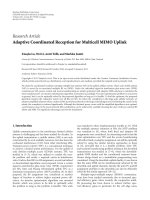
Figure 2: Polarization component 1 of a seismic signal: nonnoisy impaired results with LRTA-(8,8,3), and result with MWF-(8, 8, 3).
10
0
10
1
10
2
10
3
10

4
50 100 150 200 250 300
(a) LRFP, LRTA
10
0
10
1
10
2
10
3
50 100 150 200 250 300
(b) MWFP, MWSVD
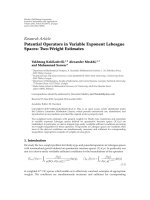
Figure 3: Computational times (s) as a function of the number of rows and columns: tensor filtering using (a) LRFP (-∗-), LRTA (-· -); (b)
MWFP (-
∗-), MWSVD (-· -).
Julien Marot et al. 9
on the required computational times. The subspace ranks are
estimated by MDL criterion unless it is specified.
A multiway white noise N which is added to signal tensor
X can be expressed as
N
= α·G, (21)
where every element of G
∈ R
I
1
×I
2
×I

3
is an independent
realization of a normalized centered Gaussian law, and where
α is a coefficient that permits to set the noise power in data
tensor R.
To evaluate quantitatively the results obtained by the pre-
sented methods, we define the signal to noise ratio (SNR, in
dB) in the noisy data tensor by SNR
= 10log(X
2
/N 
2
),
and to a posteriori verify the quality of the estimated
signal tensor, we use the normalized quadratic error (NQE)
criterion defined as follows: NQE(

X) =

X − X
2
/X
2
.
7.1. Denoising of a color image impaired by
additive noise
Let us consider the “sailboat” standard color image of
Figure 1(a) represented as a third-order tensor X
∈
R

256×256×3
. The ranks of the signal subspace for each mode
are set as 30 for the 1st mode, 30 for the 2nd mode, and
2 for the 3rd mode. This is fixed thanks to the following
process. For Figure 1(a), we took the standard nonnoisy
“sailboat” image and we artificially reduced the ranks of the
nonnoisy image, that is, we set the parameters (K
1
, K
2
, K
3
)to
(30, 30, 2), thanks to the truncation of HOSVD. This permits
to ensure that, for each mode, the rank of the signal subspace
is lower than the corresponding dimension. This also permits
to evaluate the performance of the filtering methods applied,
independently from the accuracy of the estimation of the
values of the ranks by MDL or AIC criterion.
Figure 1(b) shows the noisy image resulting from the
impairment of Figure 1(a) and represented as R
= X + N .
Third-order noise tensor N is defined by (21) by choosing α
such that, considering the definition above, the SNR in the
noisy image of Figure 1(b) is 8.1 dB. In these simulations,
the value of the parameter K of channel-by-channel SVD-
based filtering, the values of the dimensions of the row, and
column signal subspace are supposed to be known and fixed
to 30. In the same way, parameters (K
1

, K
2
, K
3
)oflower-
rank (K
1
, K
2
, K
3
) approximation are fixed to (30, 30,2). The
channel-by-channel SVD-based filtering of noisy image R
(see Figure 1(b)) yields the image of Figure 1(c), and lower-
rank (30, 30,2) approximation of noisy data tensor R yields
the image of Figure 1(d). The NQE criterion permits a
quantitative comparison between channel-by-channel SVD-
based filtering, LRTA-(30,30, 2), and MWF-(30, 30, 2). The
obtained NQE is, respectively, 0.09 with channel-by-channel
SVD-based filtering, 0.025 with LRTA-(30,30, 2), and 0.01
with MWF-(30, 30, 2). From the resulting image, presented
on Figure 1(d), we notice that dimension reduction leads to
a loss of spatial resolution. However, the choice of a set of
values K
1
, K
2
, K
3
which are small enough is the condition for

an efficient noise reduction effect.
Therefore, a tradeoff should be considered between noise
reduction and detail preservation. When MDL criterion
[32, 47] is applied to the left singular values of the
flattening matrices computed over the successive nth-modes,
the correct tradeoff is automatically reached. In the next
simulation, a multicomponent seismic wave is received on
a linear antenna composed of 10 sensors. The direction
of propagation of the wave is assumed to be contained in
a plane which is orthogonal to the antenna. The wave is
composed of three components, represented as signal tensor
X. Each consecutive component presents a π/2 radian phase
shift. Figure 2 represents nonnoisy component 1, impaired
component 1 (SNR
=−10 dB), the results of denoising
by LRTA-(8, 8, 3), and MWF-(8,8, 3) (NQE
= 0.8and3.8,
resp.).
7.2. Hyperspectral images: denoising results and
compared computational loads
The proposed fast lower-rank tensor approximation, that
we name lower-rank fixed point (LRFP), and the proposed
fast multiway Wiener filtering, that we name multiway
Wiener fixed point (MWFP), are compared with the versions
of lower-rank tensor approximation and multiway Wiener
filtering which use SVD, respectively, named lower-rank
tensor approximation (LRTA) and multiway Wiener SVD
(MWSVD).
The proposed and comparative methods can be applied
to any tensor data, such as color image, multicomponent

seismic signals, or hyperspectral images [6]. We exemplify
the proposed method with hyperspectral image (HSI)
denoising. The HSI data used in the following experiments
are real-world data collected by HYDICE imaging, with a
1.5 m spatial and 10nm spectral resolution and including
148 spectral bands (from 435 to 2326 nm). Then, HSI data
can be represented as a third-order tensor, denoted by R
∈
R
I
1
×I
2
×I
3
. A multiway white noise N is added to signal tensor
X. We consider HSI data with a large amount of noise,
by setting SNR
= 3dB.Weprocessimageswithvarious
number of rows and columns, to study the proposed and
compared algorithm speed as a function of the data size.
Each band has from I
1
= I
2
= 20 to 256 rows and columns.
Number of spectral bands I
3
is fixed to 148. Signal subspace
ranks (K

1
, K
2
, K
3
) chosen to perform lower-rank (K
1
, K
2
, K
3
)
approximation are equal to (10, 10, 15). Parameter η (see
Section 6.3.1)isfixedto10
−6
, and 5 iterations of the ALS
algorithm are needed for convergence. Figure 3(a) (resp.,
(b)) provides the evolution of computational times for both
LRFP and LRTA-based (resp., MWFP and MWSVD-based)
tensor data denoising, for values of I
1
and I
2
varying between
60 and 256, in second, with a 3.0 Ghz PC running windows
(same conditions are used throughout all experiments).
Considering an image with 256 rows and columns, LRFP-
based method leads to SNR
= 17.03 dB with a computational
time equal to 68 seconds and LRTA-based method leads

to SNR
= 17.20 dB with a computational time equal to
43 minutes, 22 seconds. Then with these image sizes, and
the ratios K
1
/I
1
= K
2
/I
2
= 410
−2
,andK
3
/I
3
= 110
−1
, the
proposed method is 38 times faster, yielding SNR values that
differ by less than 1%. MWFP-based method leads to SNR
=
17.11 dB with a computational time equal to 36 seconds and
10 EURASIP Journal on Advances in Signal Processing
250
200
150
100
50

50 100 150 200 250
(a) Raw HSI data
250
200
150
100
50
50 100 150 200 250
(b) Noised HSI data
250
200
150
100
50
50 100 150 200 250
(c) denoising Result
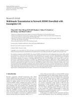
Figure 4: HSI image: results obtained by lower-rank tensor
approximation using LRFP, LRTA, MWFP, or MWSVD.
MWSVD-based method leads to SNR = 17.27 dB with a
computational time equal to 17 minutes, 4 seconds. Then,
the proposed method is 29 times faster, yielding SNR values
that differ by less than 1%. The gain in computational times
is particularly pronounced with K
1
/I
1
, K
2
/I
2

,andK
3
/I
3
ratio values which are relatively low, which is relevant for
denoising applications. Figure 4(a) is the raw image with
I
1
= I
2
= 256; Figure 4(b) provides the noised image;
Figure 4(c) is the denoising result obtained by the LRTA
algorithm. Results obtained with LRFP, MWFP, or MWSVD
algorithms look very similar.
8. CONCLUSION
This paper deals with tensor data denoising methods,
and last advances in this field. We review lower-rank
tensor approximation (LRTA) and multiway Wiener filtering
(MWF), and remind they yield good denoising results,
especially compared to channel-by-channel SVD-based pro-
cessing. These methods rely on tensor flattening along each
mode, and on the projection of the data upon a useful signal
subspace. We propose a synthesis of the last advances in
tensor signal processing methods. We show how the signal
subspace ranks can be estimated by statistical criteria; we
demonstrate that, by flattening tensors along main direc-
tions, output SNR is improved, and propose to use the fast
SLIDE algorithm to retrieve these main directions; we adapt
fixed-point algorithm and inverse power method to replace
the costly SVD in lower-rank tensor approximation and

multiway Wiener filtering methods, thus obtaining much
faster algorithms. We exemplify the proposed improved
methods on a seismic signal, color, and hyperspectral images.
ACKNOWLEDGMENT
The authors would like to thank the anonymous reviewers
who contributed to the quality of this paper by providing
helpful suggestions.
REFERENCES
[1] N. D. Sidiropoulos and R. Bro, “On the uniqueness of
multilinear decomposition of N-way arrays,” Journal of
Chemometrics, vol. 14, no. 3, pp. 229–239, 2000.
[2] N. D. Sidiropoulos, G. B. Giannakis, and R. Bro, “Blind
PARAFAC receivers for DS-CDMA systems,” IEEE Transac-
tions on Signal Processing, vol. 48, no. 3, pp. 810–823, 2000.
[3] M. A. O. Vasilescu and D. Terzopoulos, “Multilinear inde-
pendent components analysis,” in Proceedings of the IEEE
Computer Soc iety Conference on Computer Vision and Pattern
Recognition (CVPR ’05), vol. 1, pp. 547–553, San Diego, Calif,
USA, June 2005.
[4] D.C.Alexander,C.Pierpaoli,P.J.Basser,andJ.C.Gee,“Spa-
tial transformations of diffusion tensor magnetic resonance
images,” IEEE Transactions on Medical Imaging, vol. 20, no. 11,
pp. 1131–1139, 2001.
[5] D. Muti, S. Bourennane, and J. Marot, “Lower-rank tensor
approximation and multiway filtering,” to appear in SIAM
Journal on Matrix Analysis and Applications.
[6] D. Muti and S. Bourennane, “Multidimensional filtering based
on a tensor approach,” Signal Processing, vol. 85, no. 12, pp.
2338–2353, 2005.
[7] L. De Lathauwer, B. De Moor, and J. Vandewalle, “A multi-

linear singular value decomposition,” SIAM Journal on Matrix
Analysis and Applications, vol. 21, no. 4, pp. 1253–1278, 2000.
[8] L. De Lathauwer, B. De Moor, and J. Vandewalle, “On
the best rank-1 and rank-(R
1
, R
2
, , R
N
) approximation of
higher-order tensors,” SIAM Journal on Matrix Analysis and
Applications, vol. 21, no. 4, pp. 1324–1342, 2000.
[9]P.M.Kroonenberg,Three-Mode Principal Component Anal-
ysis: Theory and Applications,DSWOPress,Leiden,The
Netherlands, 1983.
[10] P. M. Kroonenberg and J. de Leeuw, “Principal component
analysis of three-mode data by means of alternating least
squares algorithms,” Psychometrika, vol. 45, no. 1, pp. 69–97,
1980.
Julien Marot et al. 11
[11] D. Muti and S. Bourennane, “Multiway filtering based on
fourth-order cumulants,” EURASIP Journal on Applied Signal
Processing, vol. 2005, no. 7, pp. 1147–1158, 2005.
[12] D.MutiandS.Bourennane,“Fastoptimallower-ranktensor
approximation,” in Proceedings of the 2nd IEEE International
Symposium on Signal Processing and Information Technology
(ISSPIT ’02), pp. 621–625, Marrakesh, Morocco, December
2002.
[13] D. Muti and S. Bourennane, “Multidimensional estimation
based on a tensor decomposition,” in Proceedings of the IEEE

Workshop on Statistical Signal Processing (SSP ’03), pp. 98–101,
St. Louis, Mo, USA, September-October 2003.
[14] D. Muti and S. Bourennane, “Multidimensional signal pro-
cessing using lower-rank tensor approximation,” in Proceed-
ings of the IEEE International Conference on Acoustics, Speech,
and Signal Processing (ICASSP ’03), vol. 3, pp. 457–460, Hong
Kong, April 2003.
[15] D. Muti and S. Bourennane, “Traitement du signal par
d
´
ecomposition tensorielle,” in Proceedings of the 19th GRETSI
Symposium on Signal and Image Processing,Paris,France,
September 2003.
[16] C. Eckart and G. Young, “The approximation of a matrix by
another of lower rank,” Psychometrika, vol. 1, no. 3, pp. 211–
218, 1936.
[17] D. Muti, S. Bourennane, and M. Guillaume, “SVD-based
image filtering improvement by means of image rotation,” in
Proceedings of the IEEE International Conference on Acoustics,
Speech, and Signal Processing (ICASSP ’04), vol. 3, pp. 289–292,
Montreal, Canada, May 2004.
[18] R. A. Harshman and M. E. Lundy, “The PARAFAC model for
three-way factor analysis and multidimensional scaling,” in
Research Methods for Multimode Data Analysis,H.G.Law,C.
W. Snyder Jr., J. Hattie, and R. P. McDonald, Eds., pp. 122–215,
Praeger, New York, NY, USA, 1984.
[19] J. D. Carroll and J J. Chang, “Analysis of individual differences
in multidimensional scaling via an n-way generalization of
“Eckart-Young” decomposition,” Psychometrika, vol. 35, no. 3,
pp. 283–319, 1970.

[20] J. Kruskal, “Rank, decomposition, and uniqueness for 3-way
and N-way arrays,” in Multiway Data Analysis, Elsevier/North-
Holland, Amsterdam, The Netherlands, 1988.
[21] H. A. L. Kiers, “Towards a standardized notation and termi-
nology in multiway analysis,” Journal of Chemometrics, vol. 14,
no. 3, pp. 105–122, 2000.
[22] R. Bro, Multi-way analysis in the food industry, Ph.D. thesis,
Royal Veterinary and Agricultural University, Copenhagen,
Denmark, 1998.
[23] N. D. Sidiropoulos, R. Bro, and G. B. Giannakis, “Parallel
factor analysis in sensor array processing,” IEEE Transactions
on Signal Processing, vol. 48, no. 8, pp. 2377–2388, 2000.
[24] M. Welling and M. Weber, “Positive tensor factorization,”
Pattern Recognition Letters, vol. 22, no. 12, pp. 1255–1261,
2001.
[25] A. Cichocki and R. Zdunek, “Ntflab for signal processing,”
Tech. Rep., Laboratory for Advanced Brain Signal Processing,
BSI, RIKEN, Saitama, Japan, 2006.
[26] L. R. Tucker, “Some mathematical notes on three-mode factor
analysis,” Psychometrika, vol. 31, no. 3, pp. 279–311, 1966.
[27] O. Alter and G. H. Golub, “Reconstructing the pathways of a
cellular system from genome-scale signals by using matrix and
tensor computations,” Proceedings of the National Academy of
Sciences of the United States of America, vol. 102, no. 49, pp.
17559–17564, 2005.
[28] L. De Lathauwer, Signal processing based on multilinear algebra,
Ph.D. thesis, Department of Electrical Engineering, Katholieke
Universiteit Leuven, Leuven, Belgium, September 1997.
[29] A. Smilde, R. Bro, and P. Geladi, Multi-Way Analysis: Applica-
tions in the Chemical Sciences, John Wiley & Sons, New York,

NY, USA, 2004.
[30] M. A. O. Vasilescu and D. Terzopoulos, “Multilinear image
analysis for facial recognition,” in Proceedings of the 16th
International Conference on Pattern Recognition (ICPR ’02),
vol. 2, pp. 511–514, Quebec, Canada, August 2002.
[31] H. Wang and N. Ahuja, “Facial expression decomposition,”
in Proceedings of the 9th IEEE International Conference on
Computer Vision (ICCV ’03), vol. 2, pp. 958–965, Nice, France,
October 2003.
[32] N. Renard, S. Bourennane, and J. Blanc-Talon, “Multiway
filtering applied on hyperspectral images,” in Proceedings of
the 8th International Conference on Advanced Concepts for
Intelligent Vision Systems (ACIVS ’06),LectureNoteson
Computer Science, pp. 127–137, Springer, Antwerp, Belgium,
September 2006.
[33] D. Letexier, S. Bourennane, and J. Blanc-Talon, “Nonorthog-
onal tensor matricization for hyperspectral image filtering,”
IEEE Geoscience and Remote Sensing Letters,vol.5,no.1,pp.
3–7, 2008.
[34] D. Letexier, S. Bourennane, and J. Blanc-Talon, “Main flat-
tening directions and Quadtree decomposition for multi-way
Wiener filtering,” Signal, Image and Video Processing, vol. 1, no.
3, pp. 253–265, 2007.
[35] A. Hyv
¨
arinen and E. Oja, “A fast fixed-point algorithm for
independent component analysis,” Neural Computation, vol.
9, no. 7, pp. 1483–1492, 1997.
[36] B. W. Bader and T. G. Kolda, “Algorithm 862: MATLAB tensor
classes for fast algorithm prototyping,” ACM T ransactions on

Mathematical Software, vol. 32, no. 4, pp. 635–653, 2006.
[37] I. Wirawan, K. Abed-Meraim, H. Ma
ˆ
ıtre, and P. Duhamel,
“Blind multichannel image restoration using subspace based
method,” in Proceedings of the IEEE International Conference
on Acoustics, Speech, and Signal Processing (ICASSP ’03), vol.
5, pp. 9–12, Hong Kong, April 2003.
[38] J. M. Mendel, “Tutorial on higher-order statistics (spectra) in
signal processing and system theory: theoretical results and
some applications,” Proceedings of the IEEE,vol.79,no.3,pp.
278–305, 1991.
[39] N. Yuen and B. Friedlander, “Asymptotic performance analysis
of blind signal copy using fourth-order cumulants,” Interna-
tional Journal of Adaptive Control and Signal Processing, vol.
10, no. 2-3, pp. 239–265, 1996.
[40] N. Yuen and B. Friedlander, “DOA estimation in multipath: an
approach using fourth-order cumulants,” IEEE Transactions
on Signal Processing, vol. 45, no. 5, pp. 1253–1263, 1997.
[41] H. Andrews and C. Patterson III, “Singular value decom-
position and digital image processing,” IEEE Transactions on
Acoustics, Speech and Signal Processing, vol. 24, no. 1, pp. 26–
53, 1976.
[42] H. Andrews and C. Patterson III, “Singular value decomposi-
tion (SVD) image coding,” IEEE Transactions on Communica-
tions, vol. 24, no. 4, pp. 425–432, 1976.
[43] A. Bendjama, S. Bourennane, and M. Frikel, “Seismic wave
separation based on higher order statistics,” in Proceedings
of the 1st IEEE International Conference on Digital Signal
Processing and Its Applications (DSPA ’98), Moscow, Russia,

June-July 1998.
12 EURASIP Journal on Advances in Signal Processing
[44] D. L. Donoho, “De-noising by soft-thresholding,” IEEE Trans-
actions on Information Theory, vol. 41, no. 3, pp. 613–627,
1995.
[45] S. G. Chang, B. Yu, and M. Vetterli, “Adaptive wavelet
thresholding for image denoising and compression,” IEEE
Transactions on Image Processing, vol. 9, no. 9, pp. 1532–1546,
2000.
[46] J C. Pesquet, H. Krim, and H. Carfantan, “Time-invariant
orthonormal wavelet representations,” IEEE Transactions on
Signal Processing, vol. 44, no. 8, pp. 1964–1970, 1996.
[47] M. Wax and T. Kailath, “Detection of signals by information
theoretic criteria,” IEEE Transactions on Acoustics, Speech and
Signal Processing, vol. 33, no. 2, pp. 387–392, 1985.
[48] H. K. Aghajan and T. Kailath, “Sensor array processing
techniques for super resolution multi-line-fitting and straight
edge detection,” IEEE Transactions on Image Processing, vol. 2,
no. 4, pp. 454–465, 1993.
[49] R. O. Duda and P. E. Hart, “Use of the Hough transformation
to detect lines and curves in pictures,” Communications of the
ACM, vol. 15, no. 1, pp. 11–15, 1972.
[50] J. Sheinvald and N. Kiryati, “On the magic of SLIDE,” Machine
Vision and Applications, vol. 9, no. 5-6, pp. 251–261, 1997.