Quantitative Techniques for Competition and Antitrust Analysis_4 pptx

5.1. Framework for Analyzing the Effect of Market Structure on Prices 233
where C is the total cost function describing the total costs of producing a given
level of output q
i
such that, for example,
C D
(
cq
i
C
1
2
dq
2
i
C F if q
i
>0;
0 if q
i
D 0:
In this model, beyond the first unit of production, marginal costs increase with
production and there is a limit to the efficient production scale. Solving the maxi-
mization problem describes the optimal quantity that this firm will want to supply
at each announced price:
q

i
D
8
<

:
p c
d
if p
i
q

i
 C.q

i
/ > 0 at q

i
D
p c
d
;
0 otherwise:
Next, suppose there are N symmetric active firms, each of which have produced
positive amounts so that their (the firm’s) supply function can be summarized as
q

i
D .p c/=d , we may sum to give the market supply function:
Q
Supply
Market
D N
Â

p

 c
d
Ã
:
If we further assume linear individual demands and S identical consumers so that the
market demand is Q
Demand
Market
D S.abp/ and that equilibrium price p

is determined
by the intersection of supply and demand, we may write
Q
Supply
Market
D N
Â
p

 c
d
Ã
D S.a  bp

/
D Q
Demand
Market

;
which is an equilibrium relationship that we may solve explicitly to give the
equilibrium price:
p

i
D
Nc CSda
N CSbd
:
Note, in particular, that the equilibrium price depends on N , that is the market
structure, and also on the cost and demand parameters including the size of the
market. Note also that with symmetric single-product firms, market structure can
be completely described by the number of firms. Richer models will require a more
nuanced description.
While the main aim of this section is to note that our various models imply
that price is a function of market structure, it would be nice to see an analytical
result which fits well with our intuition that prices should fall when the number
of competitors goes up. In fact, looking at the equation for the equilibrium price in
234 5. The Relationship between Market Structure and Price
price-taking environments makes it quite difficult to see immediately that a decrease
in N obviously always leads to an increase in price. Fortunately, the result is easier
to see if we consider the familiar picture with linear market supply and linear market
demand equations (we leave the reader to draw the diagram as an exercise). Reducing
N and having firms exit the market shifts the market supply curve leftward, which
will clearly generally result in an increase in equilibrium market price. In contrast,
entry will shift the aggregate market supply curve rightwards and, in so doing,
reduce equilibrium prices. For those who favor algebra, one can easily calculate the
derivative of the equilibrium price with respect to the number of firms N to see the
negative relation between the two in this example.

2
5.1.1.2 Market Structure in a Cournot Setting with Quadratic Costs
Consider next an oligopoly in which firms that entered the market compete in quan-
tities of a homogeneous good, the Cournot model. In this market exit does two
things. First, it reduces the number of firms so that total market output tends to be
reduced. Second, it increases the amount that any incumbent firm will produce due
to the shape of each individual firm’s equilibrium supply function. The net effect on
total output, and hence prices, is therefore potentially ambiguous. It depends on the
relative effect of an increase in firm output and a decrease in the number of firms.
Usually, we expect the impact of losing a firm not to be compensated for by the
expansion in output produced as a result by surviving rivals. In that case, price will
rise following the exit of an incumbent firm and fall following entry of a new player.
Let aggregate market demand be
Q D S.a bp/;
where S is the size of the market, so that the corresponding inverse aggregate demand
equation is
p.Q/ D
a
b

1
b
Q
S
:
Assuming again a quadratic cost function,
C.q
i
/ D cq
i

C
1
2
dq
2
i
C F;
and N profit-maximizing firms that exhibit the following first-order condition for
profit maximization:
p.Q/ C p
0
.Q/q
i
 C
0
.q
i
/ D 0;
where
Q D
N
X
iD1
q
i
:
2
Doing so allows us to check the conditions required on the parameters (a, b, c, d ) to ensure that the
linear supply and demand curves cross.
5.1. Framework for Analyzing the Effect of Market Structure on Prices 235

Solving this equation for q
i
, the firm’s reaction function is
3
q
i
D
S.a  bc/ 
P
j ¤i
q
j
2 C bSd
;
which in fact is identical for each i D 1;:::;N.
We use the Cournot–Nash equilibrium assumption under symmetry, which allows
us to assume that each firm will produce the same amount of output in equilibrium,
q
1
D q
2
DDq
N
D q

. The symmetry assumption implies that all N first-order
conditions are entirely identical,
q

D

S.a  bc/ .N 1/q

2 C bSd
;
and that allows us to solve them all by solving this single equation for q

. A little
more algebra allows us to express the equilibrium quantity supplied by each firm as
q

D
S.a  bc/
1 C N CbSd
:
Plugging the resulting aggregate quantity Nq

in the demand function, we can
retrieve the equilibrium market price:
p

D p.Nq

/
D p
Â
NS.a cb/
1 C N CdbS
Ã
D
a

b

1
bS
Â
NS.a cb/
1 C N CdbS
Ã
D
a
b

1
b
Â
N.a  cb/
1 C N CdbS
Ã
:
As with price-taking firms, we see that prices are generally dependent on market
structure.
The algebraic relationship between price and the number of firms is not obviously
negative. The magnitude of the actual predictions from the model will once again
depend on the assumptions about the cost symmetry of firms and the shape of the
demand. In the simple case of symmetric firms with decreasing returns to scale and
a linear demand, a reduction in the number of firms leads to a reduction in total
output and an increase in price.
3
The first-order condition can be expressed as
a

b

P
N
j ¤i
q
j
bS

1
bS
q
i
 c  dq
i
D 0 () aS 
X
j ¤i
q
j
 2q
i
 bSc  bSdq
i
D 0
from which the expression in the text immediately follows.
236 5. The Relationship between Market Structure and Price
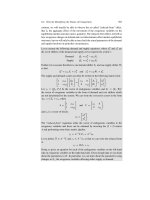
NE
p
1

p
1
p
2
NE
p
2
∗
p
1
= R
1
( p
2
; c
1
)
Price
Post merger
= Price
Cartel
p
2
= R
2
( p
1
; c
2
)

∗
p
1
= R
1
( p
2
; c
1
)
ΝΕ
ΝΕ
p
2
= R
2
( p
1
; c
2
)
ΝΕ
ΝΕ
Static ‘‘Nash equilibrium’’
prices, where each firm is
doing the best it can given
the price charged by other(s)
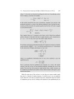
Figure 5.2. Reaction curves and static Nash equilibrium in
a two-firm industry and in a single-firm industry.
5.1.1.3 Market Structure in a Differentiated Product Price Competition Setting

As the third of our examples we now consider the case of differentiated products
Bertrand competition, in which existing firms in a market produce differentiated
products and compete in price for potential customers.
In pricing games where firms produce goods that are substitutes, optimal prices
increase in the prices of rivals under fairly weak conditions. That means that if a
firm’s rival raises its price, the best response of the firm is to also raise its own price.
The reaction functions of two firms producing substitute goods and competing in
prices are plotted in figure 5.2.
Assuming that firm 1 produces product 1 at marginal cost c
1
, the firm’s profit-
maximization problem can be expressed as
max
p
1
.p
1
 c
1
/D
1
.p
1
;p
2
IÂ/;
where D
1
.p
1

;p
2
IÂ/is the demand for product 1 and  is a consumer taste parameter.
The first-order condition for this problem can be written
@˘
Single
1
@p
1
D .p
1
 c
1
/
@D
1
.p
1
;p
2
/
@p
1
C D
1
.p
1
;p
2
/ D 0:

Solving this equation allows us to describe firm 1’s reaction function,
p

1
D R
1
.p
2
Ic
1
;Â/;
that is, its optimal choice of price for any given price of firm 2. In a similar way, we
could derive the reaction function for firm 2,
p

2
D R
2
.p
1
Ic
2
;Â/:
5.1. Framework for Analyzing the Effect of Market Structure on Prices 237
This positive relation between the optimal prices of competing firms selling sub-
stitutes is the basis for the unilateral effect described above whereby, after a merged
firm increases the prices of the substitutes goods it produces, competitors that pro-
duce other substitute goods will follow the price increase, turning this price increase
into an all-market phenomenon.
We now show analytically why a merging firm combining the production of

two substitutes has the incentive to increase both prices post-merger. This result is
derived from the fact that the merged firm can appropriate the profits generated by
the increase in the demand of the second substitute good if the price of the first good
is increased. This ability to get the profits generated by both goods will result in
higher equilibrium prices for both goods, all else equal.
Suppose we have one multiproduct firm which produces both the two goods 1 and
2. Such a multiproduct firm will solve the following profit-maximization problem:
max
p
1
;p
2
.p
1
 c/D
1
.p
1
;p
2
/ C .p
2
 c/D
2
.p
1
;p
2
/:
The first-order conditions for this problem are

@˘
Multiproduct
@p
1
D .p
1
 c/
@D
1
.p
1
;p
2
/
@p
1
C D
1
.p
1
;p
2
/ C .p
2
 c/
@D
2
.p
1
;p

2
/
@p
1
D 0
and
@˘
Multiproduct
@p
2
D .p
1
 c/
@D
1
.p
1
;p
2
/
@p
2
C D
2
.p
1
;p
2
/ C .p
2

 c/
@D
2
.p
1
;p
2
/
@p
2
D 0:
One approach to these equations is to calculate the solution .p
Multiproduct
1
;p
Multiproduct
2
/
by solving the two simultaneous equations and then consider how those prices relate
to .p
Single
1
;p
Single
2
/.Wewill do that for a very general case in chapter 8. Here, however,
we follow a different route. Namely, instead of calculating the equilibrium prices
directly, we can instead evaluate the marginal profitability of increasing prices to
the multiproduct firm at the prices .p
Single

1
;p
Single
2
/ that would have been chosen by
two single-product firms. Doing so allows us to evaluate whether the multiproduct
firm will have an incentive to raise prices. Note that we can write
@˘
Multiproduct
.p
Single
1
;p
Single
2
/
@p
1
D 0 C .p
Single
2
 c/
@D
2
.p
Single
1
;p
Single
2

/
@p
1
and
@˘
Multiproduct
.p
Single
1
;p
Single
2
/
@p
2
D .p
Single
1
 c/
@D
1
.p
Single
1
;p
Single
2
/
@p
2

C 0
238 5. The Relationship between Market Structure and Price
since at p
i
D p
Single
i
profits on the single product are maximized and the first-order
condition for single-product maximization holds. So,
sign
Â
@˘
Multiproduct
.p
Single
1
;p
Single
2
/
@p
1
Ã
D sign
Â
@D
2
.p
Single
1

;p
Single
2
/
@p
1
Ã
and
sign
Â
@˘
Multiproduct
.p
Single
1
;p
Single
2
/
@p
2
Ã
D sign
Â
@D
1
.p
Single
1
;p

Single
2
/
@p
2
Ã
:
These equations give us an important result, namely that if goods are demand
substitutes, so that
@D
1
.p
Single
1
;p
Single
2
/
@p
2
>0 and
@D
2
.p
Single
1
;p
Single
2
/

@p
1
>0;
then this “two-to-one” merger will very generally result in higher prices for both
goods. For example,
@˘
Multiproduct
.p
Single
1
;p
Single
2
/
@p
1
>0
means that the multiproduct firm will have higher profits if she raises the price of
good 1 above the single-product price.
This incentive to raise prices is what is commonly referred to as the “unilateral”
effect, or more accurately, the unilateral incentive by merging firms to raise prices
after the merger. This incentive is created by the fact that the merged firm would
retain revenues on the consumers switching to the alternative product after a price
hike. In contrast we can also conclude that if both goods are demand complements,
then prices will usually fall following a merger.
Graphically, we can represent the unilateral effect of a two-to-one merger of firms
producing substitute goods (see figure 5.2).
The prices that result from a joint maximization of profits made on goods 1 and
2 are higher than the prices that are obtained when profits are maximized for each
one of the products separately whenever goods are substitutes.

Notice, as explained above, that this result will hold if there were other firms
in the market producing other products. If the prices p
1
and p
2
increase, other
firms will also increase the prices of their goods as long as they also have upward-
sloping reaction functions with respect to p
1
and p
2
. This in turn will further cause
a further incentive to increase in the prices of p
1
and p
2
and so on until the process
settles at higher prices for all substitutable products. How much higher the prices
are compared with a situation in which there are single-product firms will depend
on the concentration and ownership structure in the market, i.e., on which firm(s)
produce(s) which products. Generally, a more concentrated ownership structure will
lead to higher prices, everything else constant.
5.1. Framework for Analyzing the Effect of Market Structure on Prices 239
This important prediction will be more closely analyzed in the context of merger
simulations and we will formalize this result for a fairly general case in chapter 8.
Merger simulation has some disadvantages but it does have the advantage that it
allows us to explicitly model the way in which merger effects depend on the shape
of demand. By doing so carefully we can reflect both the range of choices that
the consumer faces and also the substitution opportunities that exist given the con-
sumer’s taste. Chapter 9 discusses the estimation of different models of demand

functions that are useful for merger simulation exercises.
In this section, we have illustrated how the most common theoretical frameworks
used to characterize competition predict that market structure and in particular the
number of players should be expected to affect the level of prices in the market. In
particular, in the case of price competition among substitute products, the predic-
tion of the effect of an increased concentration of ownership on the price level of
all competing products is unambiguously that price will rise. The European Com-
mission Merger Regulation explicitly mentions the case when a merger will have a
negative effect on competition, and therefore on prices, quantity, or quality, because
of the reduction in the competitive pressure that firms may face after the merger.
4
In particular, the regulation states that:
However, under certain circumstances, concentrations involving the elimination
of important competitive constraints that the merging parties had exerted on each
other, as well as a reduction of competitive pressure on the remaining competitors,
may, even in the absence of a likelihood of coordination between the members of
the oligopoly, result in a significant impediment to competition.
In practice, the nature and extent of the resulting price change is an empirical ques-
tion that needs to be addressed using the facts relevant to each case. Not all mergers
will be between firms producing particularly close substitutes and some may even
involve mergers between firms producing complements. As a result, the magnitude
of the likely impact of market structure on prices must be evaluated. In what follows,
we describe several methods to empirically determine the relevance of the relation-
ship between market structure and price in specific cases. Although it will not always
be possible to perform such detailed quantitative assessments, these techniques high-
light the type of evidence that will be relevant for a unilateral effect case and provide
guidance on how to assess market evidence even when less quantitative in nature.
5.1.2 Cross-Sectional Evidence on the Effect of Market Structure
One way to look at the possible relation between market structure and prices is to
look at the market outcomes (e.g., prices) in situations where the market structure

differs. That is, an intuitive approach to evaluating whether a “three-to-two” merger
4
EC Merger Regulation, Council Regulation on the control of concentrations between undertakings
2004/1.
240 5. The Relationship between Market Structure and Price
will affect prices is to examine a market or set of markets where all three firms
compete and then look at another market or set of markets where just two firms
compete. By comparing prices across the markets we might hope to see the effect of
a move from having three active competitors to having just two active competitors.
As we will see, such a method while intuitive does need to be applied with great
care in practice since it will involve comparing markets that may be intrinsically
different. That said, if we do have data on markets with differing numbers of active
suppliers, looking at whether there is a negative correlation between the number of
firms and the resulting market prices is likely to be a good starting point for analysis.
5.1.2.1 Using Cross-Sectional Information
Using cross-sectional information can be a good starting point for an empirical
assessment of the effect of market structure on prices, provided that one can argue
that the different markets that are being compared are at least broadly similar in terms
of cost structure and demand. Consider a somewhat extreme but illustrative example.
Suppose we want to analyze the effect of the number of bicycle shops on the price of
bicycles in Beijing. It is pretty unlikely to be very helpful to use data about the price
of bicycles in Stockholm, which has fewer bicycle shops, to address the impact of
bicycle shop concentration on bicycle prices. Stockholm would have fewer shops
and higher prices than Beijing. Even ignoring the likely massive cross-country dif-
ferences in regulatory environment, the probably huge differences in tastes, market
size, and the likely differences in the cost and quality of the bikes involved, the
comparison would be effectively meaningless. No matter how concentrated Bei-
jing’s market became, there is no obvious reason to believe that equilibrium prices
would provide a meaningful comparison with Stockholm’s prices for the purposes
of evaluating mergers in either Stockholm or Beijing. Even comparing Paris and

Amsterdam, where more people favor bicycles as a mean of transportation, may
well not be appropriate.
The lesson is that when comparing prices across markets we need to make sure
that we are comparing meaningfully similar markets. With that important caveat in
mind, there are nonetheless many cases in which cross-market comparisons will be
indicative of the actual link between the number of firms competing and the price.
One famous U.S. case in which this method, along with more sophisticated meth-
ods, was used involved the proposed merger between Staples and Office Depot.
5
This
merger was challenged by the FTC in 1997.
6
The resulting court case was reputedly
5
The discussion of FTC v. Staples in this chapter draws heavily on previous discussion in the literature.
See, in particular, those involved in the case (Baker 1999; Dalkir and Warren-Boulton 1999) and also
Ashenfelter et al. (2006). There is some debate as to the extent of the reliance of the court on the
econometric evidence. See Baker (1999) for the view that econometrics played a central role. Others
emphasize that the econometrics was supplementary to more traditional documentary evidence and
testimony.
6
Federal Trade Commission v. Staples, Inc., 970 F. Supp. 1066 (United States District Court for the
District of Columbia 1997) (Judge Thomas F. Hogan).
5.1. Framework for Analyzing the Effect of Market Structure on Prices 241
the first in the United States in which a substantial amount of econometric analysis
was used by the court as evidence. The merging parties sold office supplies through
very large shops (hence they are among the set of retailers known as “big box”
retailers) and operated as specialist retailers, at least in comparison with a general
department store. Their consumers were mostly small and medium size enterprises
which are too small to establish direct relations with the original manufacturers as

well as individuals. The FTC proposed that the market should be defined as “con-
sumable office supplies sold through office superstores.” Examples of consumable
office supplies include paper, staplers, envelopes, and folders. This market definition
was somewhat controversial since it (i) excluded durable goods such as computers
and printers sold in the same stores since they are “nonconsumable,” (ii) excluded
consumable office supplies sold in smaller “mom and pop” stores, in supermarkets,
and in general mass merchants such as Walmart (not specialized office superstores).
To those skeptical about this market definition, the FTC’s lawyers suggested gently
to the judge that “one visit [to an office superstore] would be worth a thousand
affidavits.”
7
Since we have considered extensively the process of getting to market
definition in an earlier chapter, we will leave the discussion of market definition
and instead focus on the empirical evidence that was presented. While some of the
empirical evidence is relevant to market definition, its focus was primarily on mea-
suring the competitive pricing effects of a merger. The geographical market was
deemed to be at the Metropolitan Statistical Area (MSA) level, which is a relatively
local market consisting of a collection of counties.
8
By 1996, there were only three main players on the market: Staples, with a $4
billion revenue of which $2 billion was in office supplies and 550 stores in 28 states;
Office Depot, with a $6.1 billion revenue of which $3 billion was in office supplies
and 500 stores in 38 states; Office Max, with a $3.2 billion revenue of which $1.3
billion was in office supplies and 575 stores in 48 states. The merger far exceeded
the threshold for scrutiny in the United States in terms of HHI and market shares,
at least given the market definition.
The FTC undertook to compare the prices across local markets across the United
States at a given point in time to see whether there was a relationship between
the number of suppliers present in the market and the prices being charged. They
used three different data sources for this exercise. The first data set came from

internal documents, particularly Staples’s “1996 Strategy Update.” The second data
set contained prices at the SKU (product) level for all suppliers. The last data set
7
The evidence suggests Judge Hogan did indeed drive around visiting different types of stores such
as Walmart, electronics superstores, and other general supplies stores. He concluded that “you certainly
know an office superstore when you see one” and accepted the market of office supplies sold in office
superstores as a relevant “submarket.” See Staples, 970 F. Supp. at 1079 also cited in Baker and Pitofsky
(2007).
8
Some MSAs are nonetheless quite large. For example, the Houston Texas MSA is about 150 miles
(around 240 km) across.
242 5. The Relationship between Market Structure and Price
Table 5.1. Informal internal across-market price comparison.
Benchmark Comparison: Price
market structure OSS market structure reduction
Staples only Staples + Office Depot 11.6%
Staples + Office Max Staples + Office Max + Office Depot 4.9%
Office Depot only Office Depot + Staples 8.6%
Office Depot + Office Max Office Depot + Office Max + Staples 2.5%
Source: Dalkir and Warren-Boulton (1999). Primary source: Staples’s “1996 Strategy Update.”
was a survey with a comparison of average prices for a basket of goods as well as
specific comparisons for given products.
The first set of cross-market comparisons came from the parties’ internal strategy
documents. The advantage of internal strategy documents that predate the merger
is that they consist of data produced during the normal course of business and, in
particular, not as evidence “developed” to help smooth the process of approval of the
mergerbeing considered. If the firm needs the information ina particular document to
be reliable because it intends to make decisions involving large amounts of money by
using them, then it will usually be appropriate to give such documents considerable
evidential weight. In particular, such documents should probably receive far more

weight as evidence than protestations given during the course of a merger inquiry,
where there can be a clear incentive to present the case in a particular light. In this
case, the internal strategy documents provided an informal cross-market comparison
of prices by market structure. The results are presented in table 5.1 and suggest
that when markets with only Staples in are compared with markets with Staples
and Office Depot stores in, then prices are 11.6% lower in the less concentrated
market.
In addition to the internal documents, the FTC also examined advertised prices
from local newspapers in order to develop price comparisons across markets. In
particular, the FTC performed a comparison of Office Depot’s advertised prices using
the cover page of a January 1997 local Sunday paper supplement. In doing so the
FTC tried to choose two markets which provided an appropriate comparison. Ideally,
such markets will be identical except for the fact that one market is concentrated
while the other is less concentrated. In some regards it is easy to find “similar”
markets; for instance, we can fairly easily find markets of similar population to
compare. However, at the front of our minds in such an exercise is the concern that
if two markets are identical, then why do we see such different market structures?
With that caveat firmly in mind, the results are provided in table 5.2 and show
considerably higher prices in the market where there is no competition from other
office supply superstores.
5.1. Framework for Analyzing the Effect of Market Structure on Prices 243
Table 5.2. Price comparison across markets.
Orlando, FL Leesburg, FL Percentage
(three firms) (Depot only) difference
Copy paper $17.99 $24.99 39%
Envelopes $2.79 $4.79 72%
Binders $1.72 $2.99 74%
File folders $1.95 $4.17 114%
Uniball pens $5.75 $7.49 30%
Source: Figure 2 in plaintiff’s “Memorandum of points and authorities in support of motions for

temporary restraining order and preliminary injunction.” Public brief available at www.ftc.gov.os/
1997/04/index.shtm.
5.1.2.2 Comparing Price Levels of Multiple Products across Markets
Whenever an authority compares prices across multiproduct retailers the investi-
gator immediately runs into the problem of determining which prices should be
compared. If there are thousands of products being compared, it is important that
parties to the merger evaluation do not have the flexibility to pick the most favorable
comparisons and ignore the rest. In this section we consider the element of the stud-
ies which explicitly recognized the multiproduct nature of the cross-market pricing
comparisons.
The third cross-market study in the Staples case used a Prudential Securities
pricing survey which compared prices in Totawa, New Jersey (a market with three
players), with prices in Paramus, New Jersey (a market with two players). Since it
was difficult to compare prices of 5,000 with 7,000 items, it built a basket of general
office supplies that included the most visible items on which superstores usually
offer attractive prices. It found that on the “most visible” items, prices were 5.8%
lower in the three-player market than in the two-player market.
When comparing price levels across retailers or across multiproduct firms, one is
always faced with the problem of trying to measure a price level relating to many
products, often thousands of products. Sometimes, the different firms or suppliers
will not offer the same products exactly or the same combination of products so that
the comparison is not straightforward. A possible solution is indeed to construct a
basket of products for which a price index can be calculated. A famous example of
a price index is the Stone price index, named after Sir Richard Stone, which can be
calculated for a single store s using the formula
ln P
st
D
J
X

j D1
w
jst
ln p
jst
;
where w
jst
is the expenditure share and p
jst
is the price of product j in store s at
time t. This formula gives a price index for each store and its value will depend on
244 5. The Relationship between Market Structure and Price
the product mix sold in that particular store. For the purpose of comparing prices
across stores, we may therefore prefer to use an index where the weights do not
depend on the store-specific product mix, but rather depend on the general share of
expenditure within a market, such as
ln P
st
D
J
X
j D1
w
jt
ln p
jst
;
where w
jt

is the expenditure share of product j in the market rather than at the
particular store. Naturally, there is a great deal of scope for arguments with parties
about the “right” price index.
9
One could, for instance, reasonably argue for keeping
the composition of the basket constant over time as price increases might make
people switch to cheaper products. In such a case, the price index would not capture
all price increases and would also not necessarily reveal the loss in quality. In the FTC
v. Staples case, the FTC reportedly solved the choice of index by choosing one which
the opposing side’s expert witness had himself proposed, thereby making it rather
difficult to critique the choice of index too much. Such a strategically motivated
choice may not always be available and, even if it were, may not be desirable since
there is quite an extensive literature on price indices, not all of which are equally
valid in all circumstances.
Discussions about the “right” price index to use can appear esoteric to nonspecial-
ists and therefore a general rule is probably to check that conclusions are robust by
exploring the data using a few different indices. Doing so will also have the advan-
tage of helping the investigator understand the patterns in the data if she reflects
carefully on any substantive differences that arise.
To construct price indices that are representative, extensive data are needed cov-
ering a large range of products and suppliers. Price data can be obtained through a
direct survey by the investigators as long as the suppliers are unaware of the action,
or the investigatory authority is clear there are no incentives to strategically manip-
ulate observed prices. Alternatively, one could solicit internal company documents
that may provide own-price listings of products at different points of time in dif-
ferent stores or markets. Firms do tend to have documents (and databases) with
comprehensive list prices. Unfortunately, in some industries, list prices are only
weakly related to actual prices once rebates and discounts are taken into account.
If such discounts are important in the industry, it is usually advisable to take them
into account when calculating the final net price. Allocating rebates to the sales can

be a challenging exercise and one should not hesitate to ask companies for the data
and clarification as to what rebates apply to which sales. Sometimes, the quality of
the data will determine the level of minimum aggregation possible with respect to
the products and the time unit used. Finally, one should also inquire about internal
9
For a review of the price index literature, see, for example, Triplett (1992) and also Kon¨us (1939),
Frisch (1936), and Diewert (1976). For a recent contribution, see Pakes (2003).
5.1. Framework for Analyzing the Effect of Market Structure on Prices 245
documents on market monitoring as very often those will reveal relevant information
about competitors’ observed behavior.
Unless our price data come from internal computer records generated ultimately
from the point of sale, the investigative team is unlikely to have either quan-
tity or expenditure data. Unfortunately, such data are often important for price
comparisons—either for computing price indices explicitly or more generally help-
ing to provide the investigators with appropriate weighting to evidence about par-
ticular price differences. If a price comparison suggests a problem but the prices
involve goods which account for 0.000 01% of store sales, probably not too much
weight should be given to that single piece of evidence taken alone. On the other
hand, it may be possible to examine the prices associated with a relatively small
numbers of goods whose sales are known to account for a large fraction of sales.
In 2000, the U.K. Competition Commission
10
(CC) undertook a study of the
supermarket sector.
11
Several data sources were used to compare the prices of spe-
cific products and of a basket of products across chains and stores. To construct the
basket, the CC asked the twenty-four multiple grocery retailers such as Tesco, Asda,
Sainsbury’s, Morrisons, Aldi, M&S, and Budgens for details of prices charged for
200 products in 50–60 stores for each company on one particular day before the start

of the inquiry: Thursday, January 28, 1999. The basket was constructed using 100
products from the top 1,000 sales lines, picking “well-known” products across each
category and 100 products chosen at random from the next 7,000 products “although
the choices were then adjusted as necessary to reflect the range of reference prod-
uct categories.”
12
The main difficulty was comparability: finding “similar” products
sold across all supermarket chains. The CC also asked for sales revenue data for
each product in order to construct sales-weighted price indices.
The inquiry also used internal company documents in which firms monitored the
price of competitors. Aldi, for instance, had daily price checks on major competitors
as well as weekly, monthly, and quarterly reports on prices of certain goods for
selected competitors and across the whole range in discounters. Asda had three
different weekly or monthly price surveys of competitors.
13
The aim of collecting
all these data was to compare prices across local markets with different market
structures. To accomplish this, the CC’s economics staff plotted all the stores on a
map and visually selected 50–60 stores that faced either “intense,” “medium,” or
“small” amounts of local competition. This appears to be a pragmatic if slightly
ad hoc approach with the advantage that the method did generate cross-sectional
variation. Recent developments in software for geographic positioning (known as
geographic information systems) greatly facilitate characterizing local competition.
10
In its previous guise as the U.K. Monopolies and Mergers Commission.
11
Available from www.competition-commission.org.uk/rep_pub/reports/2000/446super.htm.
12
See paragraph 2 in appendix 7.6 of the CC’s supermarket final report.
13

See appendix 7.4 of the CC’s supermarket inquiry report.
246 5. The Relationship between Market Structure and Price
As always in empirical analysis, getting the right data is a first important step.
With very high-quality data on a relevant sample, simple exercises such as the cross-
sectional comparisons can be truly revealing. In the FTC v. Staples office supplies
case, all the results from the cross-sectional comparison pointed to a detrimental
effect of concentration on prices. Markets with three suppliers are cheaper than
markets with two suppliers, which are in turn cheaper than markets with a single
supplier. This was supported by the comparison across market using different data
sources. The evidence was enough to indicate that a merger might be problematic
in terms of prices to the final consumer.
Still, although local markets in the United States (and particularly neighboring
markets such as those used for many of the comparisons) are probably close enough
for the comparisons to make sense, the merging parties still claimed that price
differences were due to cost differences in the different areas and in particular that
price differences were not caused by the lack of additional competitors. The strength
of any evidence needs to be evaluated and the “cost difference” critique suggests
that the cross-market correlation between market structure and prices may be real
but the explanation for the correlation may not be market power. To address this
potentially valid critique, the FTC undertook further econometric analysis to take
account of possible market differences, and it is to that we now turn.
5.1.2.3 Endogeneity Problems in Cross-Sectional Analysis
Results obtained from a simple cross-sectional comparison across markets with
different market structures are informative provided the comparisons involved are
sensible. However, such studies will rarely be entirely conclusive by themselves
since they are vulnerable to the criticism that, although there might be a link between
market structure and price, this link is not causal. For example, if two markets
have in truth different costs, then we will tend to see both fewer stores and higher
prices in the high cost market. In such a situation an investigator could easily and
erroneously conclude that a merger to increase concentration would increase prices.

Such a situation is of particular difficulty since costs are often difficult to observe
and provides yet another example of an “endogeneity bias.”
To summarize the problem consider a regression equation attempting to explain
prices as a function of market structure:
p
m
D ˛ CN
m
 C "
m
;
where p
m
is the price in market m and N
m
is the number of firms in market m.
Suppose that the true data-generating process (DGP) is very closely related:
p
m
D ˛ CN
m

True
C u
m
;
with the determinants of prices other than “market structure,” N
m
, captured in the
unobserved component, u

m
. For instance, costs will affect prices but are not explic-
itly controlled for, so their effect is a component in the error term. If high costs
5.1. Framework for Analyzing the Effect of Market Structure on Prices 247
cause high u
m
and therefore high prices as well as low entry (low N
m
), then we
have EŒu
m
N
m
<0, i.e., the “random” term in the equation will not be indepen-
dent of the explanatory variable. This violates a basic condition for getting unbiased
estimates of the regression parameters using our standard technique of OLS (see
chapter 2). We will find that markets with fewer firms will be associated with higher
prices, but the true cause of the high prices is not the market structure but rather the
higher costs. One must therefore beware “false positives” when using across-market
data variation to identify the relationship between market structure and prices. False
positives are possible when there is a factor such as high cost that will positively
affect prices and that will also independently negatively affect entry and the number
of firms. If this happens, we will find a negative correlation between price and mar-
ket structure that is due to variation in costs (or other variable) and not to differences
in pricing power.
False negatives can also occur when using across-market data variation. This
happens when there is an omitted factor that increases both prices and the number
of firms in the market. For instance, a high demand for reasons we do not see (e.g.,
demographics, tastes) will result in high prices and also in a large number of firms.
In this case, we will tend to find a positive correlation between price and number of

suppliers that is due to variation in demands across markets. Again such a positive
correlation is not down to differences in pricing power, but may act to make pricing
power more difficult to identify. Specifically, we may find no correlation at all when
there is in fact a negative correlation due to pricing power. This is because the
“endogeneity” bias now acts to bias our estimate of 
True
upward—toward zero or
even above zero.
The endogeneity bias in the cross-sectional comparisons of markets with different
structures ultimately occurs when there is a component that we do not account for
that affects both prices and the number of firms or in other words it affects both
prices and entry.
To illustrate where the endogeneity concern comes from using a theoretical model,
consider the equilibrium price in a Cournot model with quadratic costs such as
described above:
p
m
D
a
m
b

1
b
Â
N
m
.a
m
 c

m
b/
1 C N
m
C dbS
m
Ã
;
where S is the size of the market, a and b are demand parameters, and c and d
are the cost parameters. The demand and costs parameters are unobserved and their
effect is therefore included in the error term of the pricing regression. In this model,
if we use the free entry assumption to solve for the equilibrium number of firms N ,
we get
N

m
D
a
m
 c
m
b
2
r
2S
m
.2 C dbS
m
/
bF

 1  dbS
m
:
248 5. The Relationship between Market Structure and Price
And the point to note is that both p and N are correlated with both demand and costs.
Thus the unobserved components of both demand and costs will both emerge in the
pricing equation’s residual and also be a determinant of the number of firms, N .
Sometimes, analysts will be able to convincingly argue that endogeneity is not an
issue. Often, it will be advisable to try to control for it. In the following section we
illustrate one way of attempting to do so.
5.1.3 Using Changes over Time: Fixed-Effects Techniques
Fixed-effects techniques were introduced in chapter 2 and are closely related to the
natural experiment techniques discussed in chapter 4.
14
In both cases, one observes
how the outcome of interest (for example price) for similar observations changes
over time following changes in the explanatory variable for only some but not all
the observations, thereby identifying the effect of that explanatory variable on the
outcome of interest. The great advantage of these techniques is that we do not need
to control for all the remaining explanatory variables that are assumed to remain
constant. Fixed effects are also technically very simple to implement. When used
properly, fixed effects are a powerful empirical method that provides solid evidence.
But as in many empirical exercises, the ability to produce regression results with
easy-to-use software can mean that the technique appears deceptively simple. In
reality, the investigator must make sure that the conditions necessary for the validity
of the method are satisfied. In this section we discuss fixed effects and highlight when
this very appealing technique may be properly used and when, on the contrary, one
must be wary of applying it.
5.1.3.1 Fixed Effects as a Solution for Endogeneity Bias
To identify the effect of market structure on the level of prices one must control

for each of the determinants of price and obtain the pure effect of the number of
competitors on price. The difficulties are both that the number of variables that one
needs to control for may be large and that at least some of the variables (particularly
cost data) are likely to be difficult to observe. Comprehensive data are therefore
unlikely to be available. One way to proceed in the face of this issue is to choose a
reasonably homogeneous subset of observations and look at the effect of the change
in market structure on that subset. For example, we may look over time at the effect
of a change in market structure affecting the price at a particular store. Such an
approach uses “within-store” and “across-time” data variation. This kind of data
variation is very different from the across-store or across-market data variation used
in the previous section to identify the relationship between prices and the number
14
The econometric analysis of fixed-effects estimators and other techniques for panel data are widely
discussed in the literature. For example, readers may wish to consult Greene (2007), Baltagi (2001), or
Hsiao (2003).
5.1. Framework for Analyzing the Effect of Market Structure on Prices 249
of stores. If we have just one store, we could use the data variation from that one
store and the only data variation would be “within store across time.” However, if
we have many stores observed over time, then we can combine the cross-sectional
information with the time series information that we have for each store. Data that
track a particular sample (of firms, individuals, or stores) over time are referred
to as panel data. Panel data sometimes offer good opportunities for identification
because we can use either cross-sectional or a cross-time data variation to identify
the effect of market structure on prices. A panel data regression model for prices
can be written
p
st
D ˛
s
C x

st
ˇ C"
st
;
where s indicates the cross-sectional index (here, the store) and t indicates the time
period so that the price p
st
is store-time specific as are the explanatory variables, x
st
.
Allowing for a store fixed effect ˛
s
in the regression controls for a particular price
level to be associated with each store. By introducing this store-specific constant and
looking at the effect of a change of structure (i.e., a variable in x
st
) on that store, we
control for all store-specific time-invariant store characteristics. For example, if our
data are fairly high frequency and costs change slowly, then the store’s cost structure
may be sufficiently constant across time for this to be a reasonable approximation.
Similarly, the fixed effect may successfully control for the impact of store character-
istics such as a particularly good location persistently affecting demand and hence
prices. Controlling for these unobserved characteristics by using the store fixed effect
will help address the concern we highlighted with the cross-sectional evidence, that,
for example, the costs in a particular location are high and this is therefore associ-
ated with both high prices and low entry. Thus store fixed effects may help alleviate
“endogeneity bias.” Such an approach to alleviate endogeneity is often used when
the researcher has panel data.
15
Of course, one still needs to account for time-varying

effects but permanent structural differences across stores are at least accounted for.
To be clear, the fixed-effects technique will only work to the extent that there is not
any substantial time-varying change in demand or costs within stores that affect both
the number of local stores and prices. If there are, then the fixed-effects approach
may not help solve the problems associated with endogeneity bias.
To illustrate this method let us return to our discussion of the FTC v. Staples/Office
Depot case. In that case, the FTC had product level data from 428 Staples stores
in 42 cities for 23 months available. To make the data set manageable, a monthly
price index was constructed for each store, based on a basket of goods. The FTC
proposed the following fixed-effects regression:
p
smt
D ˛
s
C x
smt
ˇ C"
smt
;
where as before s indicates store, t indicates the time period, m indicates market or
city, p is the price variable, and x, in this instance, is a set of dummy indicators for
15
For a review of the history of panel data econometrics, see Nerlove (2002). (See, in particular,
chapter 1 of that book, entitled “The history of panel data econometrics, 1861–1997.”)
250 5. The Relationship between Market Structure and Price
the presence of nearby stores such as an Office Depot within five miles (OD
5 miles
smt
)or
the presence of a local Walmart or other potentially relevant competitor stores. The

latter coefficients turned out to be insignificant so we will focus on the effect of the
Office Depot store. Note that the regression has a store-specific fixed effect ˛
s
, which
means that the changes in the x variables are considered “holding the store effect
constant.” Specifically, if a single store experiences nearby entry, we will see that
either its price drops or it does not. For those stores which experience no change in
prices over time, the store fixed effect will absorb all of the variation in prices and so
that variation will not be used to help identify the value of the parameters in ˇ. That
is, in contrast to the cross-sectional data variation, the store fixed-effects regression
uses primarily the “within-store” data variation, albeit using the within-store data
variation across the whole sample (see also the discussion on this point in chapter 2).
The fixed-effects regression was meaningful in this case because there was enough
informative variation in the data. Prices varied across time and across stores but it
is notable that they varied more across stores than across time. Since the store
fixed effects will account for all the time-invariant variation across stores, only the
relatively small amount of within-store data variation may be left once the fixed
effects are allowed for. Fortunately, there was some variation across time within a
store in prices and also in the presence of competitors in some of the stores’market.
Enough stores experienced entry by nearby rival stores to ensure that it was possible
to identify the effect of that change in market structure on prices.
The effect of the presence of a competitor (i.e., an Office Depot store) on Staples’s
prices can be calculated using the expression:
100
Op
smt
.OD
5 miles
smt
D 1/ Op

smt
.OD
5 miles
smt
D 0/
Op
smt
.OD
5 miles
smt
D 0/
D 100
O
ˇ
OD
Op
smt
.OD
5 miles
smt
D 0/
;
where Op
smt
.OD
5 miles
smt
D 1/ denotes the predicted price level at store s in market
m at time t when the x variable associated with the indicator for whether there is
an Office Depot within five miles takes on the value 1 and Op

smt
.OD
5 miles
smt
D 0/
is defined analogously. This expression provides the predicted percentage decrease
in prices at a Staples store which results from having an Office Depot within five
miles, all else equal.
The defendants’ expert found only a 1% effect of the presence of an office supply
superstore on the price and claimed that the difference with the cross-sectional
results was due to the endogeneity bias caused by comparing stores in different
markets.
16
He argued that the difference between the cross-sectional and fixed-
effects estimates arose because the panel data estimates controlled for store-specific
costs that were not observed directly and hence not controlled for in either the
cross-sectional regression or the panel data regression unless fixed effects were
included. However, in the event Baker (1999) argues there were several problems
16
Specifically, 100 
O
ˇ
OD
= Op
smt
.OD
5 miles
smt
D 0/ D 1%.
5.1. Framework for Analyzing the Effect of Market Structure on Prices 251

with the defendant’s expert regression. First, the FTC view was that the expert had
somewhat arbitrarily drawn circles around stores at 5 miles, 10 miles, and 20 miles
and constructed dummies for the presence of stores within that range. The FTC
argued that internal documents suggested that companies priced according to pricing
zones that were not circles and could sometimes be quite large and as large as the
MSA area. While generally an approach of drawing circles around stores would
seem a highly plausible way to proceed, the regression aims to capture the data-
generating process for prices. Here the documents reveal the nature of competitive
interaction and so the specification should be guided by the documentary evidence.
Including the count of stores within the MSA tripled the price effect to a range of
about 2.5–3.7%. Thus the FTC argued that the merging parties’ preferred results
were (1) not robust to slight changes in specification and (2) did not reflect the
documentary evidence. In addition, Baker (1999) reports that the defendant’s expert
had dropped from their sample observations from California, Pennsylvania, and a
few others for reasons that were not entirely clear. When included back in the data
set, the effect was estimated to be three times larger again, between 6.5% and 8.6%
depending on the detail of the specification. Thus in sum, the FTC expert concluded
that a reasonable estimate was that prices of Staples stores were on average 7.6%
lower when an Office Depot store was in the MSA, which was also consistent with
their findings using only cross-sectional data variation.
5.1.3.2 Limitations of Fixed Effects
Fixed-effect regressions attempt to control for the bias generated by the presence
of endogeneity or omitted explanatory variables. These problems can be potentially
severe in cross-sectional comparisons and the use of panel data provides an oppor-
tunity to at least partially address the endogeneity problem. Fixed-effect regressions
control for firm- (or store-) specific characteristics and compute the effect of a change
in the variable of interest for a particular firm (or store) only. However, because we
force the effect to be measured only within firm (or store), we are, albeit deliberately,
no longer fully exploiting the cross-sectional variation.
Suppose, for instance, that there is very little variation in market structure over

time, i.e., no entry or exit, and we estimate a specification which includes in x a
count of the number of nearby stores. When we estimate
p
st
D ˛
s
C x
st
ˇ C"
st
;
we will estimate ˇ D 0 because the store fixed effect will explain all the observed
variation in prices and there will be no additional variation in the data allowing us
to tell apart the store-specific fixed effect and the effect of local market structure,
which did not change for any given store. In an extreme case, when there is literally
no time series variation in market structure, our regression package will either fail or
else tend to print out estimates of standard errors which involve very large numbers
252 5. The Relationship between Market Structure and Price
indeed. The reason is that we have tried to estimate a model which is simply not
identified unless there is time series variation in the local market structure variables.
It is very important to realize that such a finding does not necessarily mean the
variation in prices across markets is not at least partly caused by the variation in
market structure. In our office supplies example, stores with a competitor nearby
may have lower prices and this is just showing up in the difference in the level of
the store fixed effect (˛
s
). Cross-sectional variation may be explained by omitted
variables but it might also be due to lack of competition near some stores. Thus, it
may be appropriate to consider fixed-effects estimates as low-end estimates when
most of the data variation is cross sectional.

In sum, the fixed-effects regression identifies the coefficients in ˇ by using the
variation in the data within a group of observations, for example, across time for a
given store as well as the across-store variation to the extent that the specification
restricts the slope coefficients to be the same across stores (see the extensive discus-
sion in chapter 2). If there is not enough within-store data variation, the regression
will be uninformative about slope parameters. In fact, if most of the variation in
the data is across groups because little changes within the groups, then by using
the fixed effects we effectively lose all the information in the data into the fixed
effects. One lesson is that analysts must be aware of the source of information, i.e.,
the source of the variation in the data set, when choosing the appropriate econo-
metric technique. Fixed-effect estimators will help correct an endogeneity problem
but to do so there must be sufficient within-group variation in the data. A second
lesson is that fixed-effects estimators can be used to test cross-sectional evidence
but the results must be interpreted carefully—a concern raised by a cross-sectional
relationship between market structure and price may not be allayed by a finding that
the relationship does not survive to the fixed-effects model. A mistaken belief that
is the case can mean that a case handler erroneously finds there is no problem with
a merger when in fact it is just that there is very little identifying variation in the
explanatory variables in her data set.
5.1.4 Using Time and Cross-Sectional Variation
When the variation in the data is mostly cross sectional, fixed-effects techniques that
follow a store or a firm over time may not be very informative. Moreover, we have
argued that it may be a mistake to take out all of the cross-sectional variation in the
data when evaluating the effect of a merger by introducing the fixed effects. We may
be controlling for endogeneity but in doing so we might be taking out much of the
effect of interest. As a result it will sometimes be useful to revisit cross-sectional
data variation. To do so, we can use our panel data set but carefully choose the
technique in order to ensure that we use the cross-sectional variation in the data to
identify the effect of market structure on prices appropriately.
5.1. Framework for Analyzing the Effect of Market Structure on Prices 253

5.1.4.1 Explaining the Variation in the Data
One approach is to break up the price variance in the sample into a part which varies
over time, a part which is firm or store specific, and an idiosyncratic part particular
to a time and firm or store. To do this we can run the following regression:
p
st
D ˛
s
C 
t
C "
st
;
where ˛
s
is the store-s-specific effect, 
t
is the time-t -specific component, and "
st
is the store- and time-specific component for each observation. We can then run
the store-specific effect on a set of regressors, including measures of rivalry from
competitors:
O˛
s
D x
s
ˇ Cu
s
:
This method will have the merit of exploiting all the variation in the data but if we

omit variables that are linked with the structure of competition as well as with the
price, then we will still have an endogeneity problem just as in the cross-sectional
analysis. Specifically, if the covariance between the regressors x
s
and the error
term u
s
is not zero, then OLS estimators will be biased. Assuming we have an
endogeneity problem only in one variable, then the sign of the endogeneity bias will
be the sign of covariance between the regressor and the error terms. Instrumental
variable techniques can help alleviate such biases.
5.1.4.2 Moulton Bias
Regression analysis typically assumes that every observation in the sample is inde-
pendent and identically distributed (i.i.d.). This means that observations in the sam-
ple .Y
i
;X
i
/ are independent draws from the population of possible outcomes. If we
use panel data of a cross section over time and there is little change in the variables
over time, then the observations are not really independent but are in fact closely
related. If so, then we are doing something close to drawing the same observation in
each time period. For example, suppose we have monthly data for twenty stores over
two years but that during those two years very little changes in terms of the structure
of competition and prices. The regression assumes we have 2420 D 480 different
independent observations but in fact it is closer to the truth to say that we only have
twenty independent observations since there is barely any variation over time and
the information in the data mostly comes from the cross-sectional variation across
the twenty stores. Our 480 pairs .p; N /, where p is price and N is the number of
competitors, are not i.i.d. The consequence is that the standard errors computed by

the standard formula in a regression package will underestimate the true value of
uncertainty associated with our estimates, i.e., the precision of the estimated effect
will be overstated. As a result, we are more likely to find an effect when there is in
reality not enough information to establish one. Correcting this problem involves
254 5. The Relationship between Market Structure and Price
modeling the error structure to account for the correlation across observations.
17
Alternatively, the technique described above in which we computed the predicted
cross-sectional variation in the outcome variable (prices in our example) and related
it to possible determinant of prices including the variable of interest (number of
competitors in our example) provides a way of ensuring that standard errors are
computed based on the relevant number of independent observations.
5.1.5 Summary of Good Practice
The above discussion has we hope provided a focused discussion of the challenges
of identifying price-concentration relationships. Along the way the discussion has
illustrated some important elements of good practice when attempting to use empir-
ical techniques to identify the effect of one variable on another. Because those good
practices are very important to ensure the quality of the results, we proceed to
summarize them.
Collect meaningful data. From the beginning of the investigation, it is important
to gather data on the relevant variables for a representative sample. One should not
hesitate to contrast data from different sources and check whether other evidence
such as that coming from company documents does fit the picture that emerges
from the empirical analysis.
Check that there is enough variation in the data to identify an effect. Empiri-
cal work will only be as good as the data used. If there is not a lot of variation
in the variable of interest in the sample that we examine, it will be very difficult
to determine the effect of this variable on any outcome. Variation can be cross
sectional or across time and it can be explainable or idiosyncratic. Giving con-
siderable thought to the process that is generating the data, i.e., thinking about

the determinants of the observed outcome, will be vital both in terms of under-
standing the data and also in determining the best econometric methodology to
use.
Beware of endogeneity. Once it is established that there is enough variation in
the data to estimate an effect, one must be able to argue a causal link between
the variable of interest and the outcome. In order to do this, it is important to
make sure that all other important determinants of the outcome that could bias
the coefficient of the variable of interest are controlled for. If they cannot be
controlled for, other methods of identification should be tried or else one must
explain why endogeneity is not likely to be a problem. Often it will be possible
to sign the expected bias emerging from a particular estimation technique. When
we change the estimation technique to control for endogeneity, our estimation
results should change in the expected direction.
17
See Kloek (1981) and Moulton (1986, 1990). In practice, statistical packages have options to help
correct for Moulton bias. For example, STATA has the option “cluster” to its “regress” command. For a
more technical discussion of Moulton bias, see, for example, Cameron and Trevedi (2005).
5.1. Framework for Analyzing the Effect of Market Structure on Prices 255
Perform robustness analysis. Once a regression is run, it is important to make sure
that the resulting coefficients are relatively robust to reasonable changes in the
specification. For example, results should not be crucially dependent on the exact
composition of the sample, except perhaps in deliberate or well-understood ways.
They should also not depend on a particular way of measuring the explanatory
variables unless we know for sure that it is exactly the correct way to measure
them. In general, good results are robust and show up to a higher or lesser extent
across many sensible regression specifications.
Use more than one method. One good way to generate confidence in the results
of empirical analysis is to use more than one method and show that they all tend
toward the same conclusions. If different methods produce divergent results, one
should have a convincing explanation of why this happens.

Do not treat econometric evidence as “separate” from the investigation. First,
no single source of evidence is likely to be entirely compelling and generally
econometric evidence in particular runs the risk of being treated skeptically
by judges who are extremely unlikely to be expert econometricians. That risk
increases when the results are presented as some form of a mysterious “black
box” analysis. Always look for graphs that can be drawn to illustrate the data
variation generating the econometric results. Second, when econometric analysis
proceeds in a vacuum, disconnected from the rest of the case team and hence
the facts of the case, the results are unlikely to capture the core elements of the
data-generating process and, as a result, the analysis is fairly unlikely to be either
particularly helpful or robust.
In our case study, the FTC’s evaluation of the merger of office supplies superstores,
the FTC did manage to produce convincing evidence that the number of players and
the prices were negatively related. The summary of their findings is presented in
table 5.3.
This table presents as convincing a case that the merger between the two super-
stores will increase prices by more than 5% as is likely to arise in practical case
settings. The results are consistent and robust and therefore easy for a nonspecialist
judge to accept as credible. In fact, on June 30, 1997, the FTC got a federal district
court judge to grant a preliminary injunction blocking the proposed merger between
Staples and Office Depot. Subsequently, the parties gave up on their merger plans.
That sounds like good news for empirical work in antitrust. However, before coming
to that view it is very important for all to realize that such activity probably cannot
become the benchmark for the level of evidence required by antitrust authorities in
all but the most important cases. The fact that the analysis in Staples took two expert
witnesses and about six Ph.D. economists to undertake means it is resource intensive.
While the first time will always be harder than the second and third times, the decision
256 5. The Relationship between Market Structure and Price
Table 5.3. Estimating merger effects using different sources.
Estimated price

Forecasting method increase from merger
Noneconometric forecast: 5–10%
internal strategy documents
Estimate from simple comparisons of average 9%
price levels in cities where Staples
does/does not compete with Office Depot
Cross-section, controlling for the presence of 7.1%
nonsuperstore retailers
Fixed effects, with nonsuperstore retailers in 7.6%
Weighted average of two regional estimates 9.8%
(California and rest of United States)
Source: FTC results from a variety of specifications as reported in Baker (1999).
in the more recent Ryanair and Aer Lingus case
18
(which provides a European
example of such analysis) runs to more than five hundred pages of careful analysis.
5.2 Entry, Exit, and Pricing Power
In the previous section, we discussed some techniques for determining the impact
that market structure has on the level of prices.A great deal of our discussion revolved
around the problem of endogeneity, or the fact that the number of firms is potentially
not exogenously determined but rather is determined in part by the expected profits
that firms think they would make if they enter, and this in turn may be related to
prices. Cost and demand factors may simultaneously affect both prices and structure.
In simple economic models of the world where entry is assumed relatively unfettered
by barriers, high profits will attract entry, which in turn induces higher market output
and lower prices. If entry is relatively free, we will expect the process of competition
to work, driving prices down to the great benefit of consumers. That said, there is a
variety of sources of barriers to entry. Some entry barriers are natural—you cannot
enter the gold-mining business unless you have access to gold deposits. Some entry
barriers are regulatory—you cannot enter the market for prescribing drugs without

the requisite qualifications.
19
On the other hand, oligopolistic firms may strategically
18
Case no. Comp/M.4439. Thisdecisionisavailable at />cases/decisions/m4439
20070627
20610 en.pdf. See, in particular, Annex IV: Regression analysis
technical report.
19
Of course, such regulatory barriers may aim to solve another problem. Free entry into prescription
writing may reduce the costs of getting a prescription for a patient, but one might worry both about the
suitability of the resulting prescriptions and the total costs of prescribing if the patient’s cost of drugs is
subsidized by a national health care system.
5.2. Entry, Exit, and Pricing Power 257
seek to raise entry barriers and thereby deter entry. For example, firms may try to
influence the perceived profits by potential entrants in a way that may deter such
entry even if the existing firm is making substantial profits. This section turns to the
analysis of entry and potential entry and examines in particular the way in which
strategic entry deterrence may take place. In doing so, we hope to illustrate how to
inform the sometimes difficult question of whether entry is likely to play the role of
an effective disciplinary force.
5.2.1 Entry and Exit Decisions
Entry is the first decision a firm faces. Entering a market involves investment in
assets and at least a portion of those investment costs will typically become sunk
costs. On the other hand, a firm may choose not to enter and by doing so will save
the sunk costs and leave its resources available for other purposes. The simplest
model of firm entry behavior therefore posits that a firm will enter a market if the
net profits obtained from doing so are at least as large as the best alternative use of its
capital. Of course, since sunk costs incurred on entry today will typically generate
a stream of profits over some future time horizon, when estimating net profits, we

will often want to consider the net present value of the stream of profits it hopes to
generate in the future. Such an approach will be familiar to accountants in the form
of discounted cash flow (DCF) approaches to evaluating profit opportunities and to
financial analysts evaluating whether stocks are appropriately valued. The difference
with standard accounting and financial market practice here is that we must typically
study such entry opportunities in strategic environments. To that end, in this section
we study methods which may help us to analyze such strategic situations.
We begin by studying a practical example for a two-firm game in which each
firm must, like an entry game, makea1or0decision—in this case to exit or stay
in the market. Exactly the same methods can apply to the analysis of entry games,
although the data required are necessarily more prospective if a firm has not yet
decided to enter the market. After this illustrative example, we return to consider
the entry game.
For illustration, consider the competition
20
between two air carriers Prime Air and
Lean Air considering entering an intercontinental route. Assume initially, Prime Air
was awarded the only available slots to link both airports. Having been awarded
a monopoly, Prime Air expects to make handsome profit. However, Lean Air
announces shortly after that it will also start flying to a sufficiently close airport
that has refurbished its facilities for international flights. Prime Air management
had thought that the airport in question was too small and remote so that the entry
20
The observant reader will detect that this is a fictional example, but it is one that has parallels in
numerous real-world cases, particularly in the airline industry and local bus markets. For a wonderful and
richly historical illustration of these kinds of calculations in a practical setting, see the Harvard Business
School case, British Sky Broadcasting versus Sky Television (HBS case number 5-799-078).