Quantitative Techniques for Competition and Antitrust Analysis_2 ppt

1.2. Technological Determinants of Market Structure 23
0
100
200
300
400
500
1899 1902 1905 1908 1911 1914 1917
1920
Relative capital stock, 1899 = 100
Relative number of workers, 1899 = 100
Index of manufacturing production, 1899 = 100
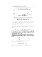
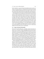
Figure 1.8. A plot of Cobb and Douglas’s data.
in the United States between 1899 and 1924. Their time series evidence examines
the relationship between aggregate inputs of labor and capital and national output
during a period of fast growing U.S. labor and even faster growing capital stock.
Their data are plotted in figure 1.8.
20
Cobb and Douglas designed a function that could capture the relationship between
output and inputs while allowing for substitution and which could be both empiri-
cally relevant and mathematically tractable. The Cobb–Douglas production function
is defined as follows:
Q D a
0
L
a
L
K
a
K
u H) ln Q D ˇ

0
C a
L
ln L C a
K
ln K C v;
where v D ln u, ˇ
0
D ln a
0
, and where the parameters .a
0
;a
L
;a
K
/ can be eas-
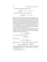
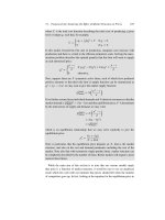
ily estimated from the equation once it is log-linearized. As figure 1.9 shows, the
isoquants in this function exhibit a convex shape indicating that there is a certain
degree of substitution among the inputs.
Marginal products, the increase in production achieved by increasing one unit of
an input holding other inputs constant, are defined as follows in a Cobb–Douglas
function:
MP
L
Á
@Q
@L
D a
0

a
L
L
a
l
1
K
a
K
F
a
F
u D a
L
Q
L
;
MP
K
Á
@Q
@K
D a
0
L
a
l
a
K
K

a
K1
F
a
F
u D a
K
Q
K
;
so that the marginal rate of technical substitution is
MRTS
LK
D
@Q=@L
@Q=@K
D
a
L
a
K
K
L
:
20
In their paper (Cobb and Douglas 1928), the authors report the full data set they used.
24 1. The Determinants of Market Outcomes
L
K
Q

1
Q
2
Q
3
Figure 1.9. Example of isoquants for a Cobb–Douglas function.
0
1.0
1899 1901 1903 1905 1907 1909 1911 1913 1915 1917 1919 1921
Year
Marginal product of labor Marginal product of capital
1.2
0.8
0.6
0.4
0.2
1922
Figure 1.10. Cobb and Douglas’s implied marginal products of labor and capital.
Cobb and Douglas’s econometric evidence suggested that the increase in labor
and particularly capital over time was increasing output, but not proportionately. In
particular, as figure 1.10 shows their estimates suggested that the marginal product
of capital was declining fast. Naturally, such a conclusion in 1928 would have
profound implications for the likelihood of continued large capital flows into the
United States.
1.2.2 Cost Functions
A production function describes how much output a firm gets if it uses given levels of
inputs. We are directly interested in the cost of producing output, not least to decide
how much to produce and as a result it is quite common to estimate cost functions.
1.2. Technological Determinants of Market Structure 25
Rather surprisingly, under sometimes plausible assumptions, cost functions contain

exactly the same information as the production function about the technical possi-
bilities for turning inputs into outputs but require substantially different data sets
to estimate. Specifically, assuming that firms minimize costs allows us to exploit
the “duality” between production and cost functions to retrieve basically the same
information about the nature of technology in an industry.
21
1.2.2.1 Cost Minimization and the Derivation of Cost Functions
In order to maximize profits, firms are commonly assumed to minimize costs for
any given level of output given the constraint imposed by the production function
with regards to the relation between inputs and output. Although the production
function aims to capture the technological reality of an industry, profit-maximizing
and cost-minimizing behaviors are explicit behavioral assumptions about the ways
in which firms are going to take decisions. As such those behavioral assumptions
must be examined in light of a firm’s actual behavior.
Formally, cost minimization is expressed as
C.Q;p
L
;p
K
;p
F
;uI˛/ D min
L;K;F
p
L
L C p
K
K C p
F
F

subject to Q 6 f.L;K;F;uIa/;
where p indicates prices of inputs L, K, and F , u is an unobserved cost efficiency
parameter, and ˛ and a are cost and technology parameters respectively. Given
input prices and a production function, the model assumes that a firm chooses the
quantities of inputs that minimize its total cost to produce each given level of output.
Thus, the cost function presents the schedule of quantity levels and the minimum
cost necessary to produce them.
An amazing result from microeconomic theory is that, if firms do indeed (i) min-
imize costs for any given level of output and (ii) take input prices as fixed so that
these prices do not vary with the amount of output the firm produces, then the cost
function can tell us everything we need to know about the nature of technology.As a
result, instead of estimating a production function directly, we can entirely equiva-
lently estimate a cost function. The reason this theoretical result is extremely useful
is that it means one can retrieve all the useful information about the parameters of
technology from available data on costs, output, and input prices. In contrast, if we
were to learn about the production function directly, we would need data on output
and input quantities.
This equivalency is sometimes described by saying that the cost function is the
dual of theproductionfunction, in the sensethatthere is a one-to-one correspondence
21
This result is known as a “duality” result and is often taught in university courses as a purely
theoretical equivalence result. However, we will see that this duality result has potentially important
practical implications precisely because it allows us to use very different data sets to get at the same
underlying information.
26 1. The Determinants of Market Outcomes
between the two if we assume cost minimization. If we know the parameters of the
production function, i.e., the input and output correspondence as well as input prices,
we can retrieve the cost function expressing cost as a function of output and input
prices.
For example, the cost function that corresponds to the Cobb–Douglas production

function is (see, for example, Nerlove 1963)
C D kQ
1=r
p
˛
L
=r
L
p
˛
K
=r
K
p
˛
F
=r
F
v;
where v D u
1=r
, r D ˛
L
C ˛
K
C ˛
F
, and k D r.˛
0
˛

˛
L
L
˛
˛
K
K
˛
˛
F
F
/
1=r
.
1.2.2.2 Cost Measurements
There are several important cost concepts derived from the cost function that are of
practical use.
The marginal cost (MC) is the incremental cost of producing one additional unit
of output. For instance, the marginal cost of producing a compact disc is the cost of
the physical disc, the cost of recording the content on that disc, the cost of the extra
payment on royalties for the copyrighted material recorded on the disc, and some
element perhaps of the cost of promotion. Marginal costs are important because
they play a key role in the firm’s decision to produce an extra unit of output. A
profit-maximizing firm will increase production by one unit whenever the MC of
producing it is less than the marginal revenue (MR) obtained by selling it. The
familiar equality MC D MR determines the optimal output of a profit-maximizing
firm because firms expand output whenever MC < MR thereby increasing their total
profits.
A variable cost (VC) is a cost that varies with the level of output Q, but we shall
also use the term “variable cost” to mean the sum of all costs that vary with the

level of output. Examples of variable costs are the cost of petrol in a transportation
company, the cost of flour in a bakery, or the cost of labor in a construction company.
Average variable cost (AVC) is defined as AVC DVC=Q. As long as MC < AVC,
average variable costs are decreasing with output. Average variable costs are at a
minimum at the level of output at which marginal cost intersects average variable
cost from below. When MC > AVC, the average variable costs is increasing in
output.
Fixed costs (FC) are the sum of the costs that need to be incurred irrespective
of the level of output produced. For example, the cost of electricity masts in an
electrical distribution company or the cost of a computer server in a consulting firm
may be fixed—incurred even if (respectively) no electricity is actually distributed or
no consulting work actually undertaken. Fixed costs are recoverable once the firm
shuts down usually through the sale of the asset. In the long run, fixed costs are
frequently variable costs since the firm can choose to change the amount it spends.
That can make a decision about the relevant time-horizon in an investigation an
important one.
1.2. Technological Determinants of Market Structure 27
Sunk costs are similar to fixed costs in that they need to be incurred and do not
vary with the level of output but they differ from fixed costs in that they cannot
be recovered if the firm shuts down. Irrecoverable expenditures on research and
development provide an example of sunk costs. Once sunk costs are incurred they
should not play a role in decision making since their opportunity cost is zero. In
practice, many “fixed” investments are partially sunk as, for example, some equip-
ment will have a low resale value because of asymmetric information problems or
due to illiquid markets for used goods. Nonetheless, few investments are literally
and completely “sunk,” which means informed judgments must often be made about
the extent to which investments are sunk.
In antitrust investigations, other cost concepts are sometimes used to determine
cost benchmarks against which to measure prices. Average avoidable costs (AAC)
are the average ofthecosts per unit that could have been avoided if acompany hadnot

produced a given discrete amount of output. It also takes into account any necessary
fixed costs incurred in order to produce the output. Long-run average incremental
cost (LRAIC) includes the variable and fixed costs necessary to produce a particular
product. It differs from the average total costs because it is product specific and does
not take into account costs that are common in the production of several products.
For instance, if a product A is manufactured in a plant where product B is produced,
the cost of the plant is not part of the LRAIC of producing A to the extent that it is
not “incremental” to the production of product B.
22
Other more complex measures
of costs are also used in the context of regulated industries, where prices for certain
services are established in a way that guarantees a “fair price” to the buyer or a “fair
return” to the seller.
In both managerial and financial accounts, variable costs are often computed and
include the cost of materials used. Operating costs generally also include costs of
sales and general administration that may be appropriately considered fixed. How-
ever, they may also include depreciation costs which may be approximating fixed
costs or could even be more appropriately treated as sunk costs. If so, they would
not be relevant for decision-making purposes. The variable costs or the operating
costs without accounting depreciation are, in many cases, the most relevant costs for
starting an economic analysis but ultimately judgments around cost data will need
to be directly informed by the facts pertinent to a particular case.
22
For LRAIC, see, for example, the discussion of the U.K. Competition Commission’s inquiry in
2003 into phone-call termination charges in the United Kingdom and in particular the discussion of the
approach in Office of Fair Trading (2003, chapter 10). In that case, the question was how high the price
should be for a phone company to terminate a call on a rival’s network. The commission decided it was
appropriate that it should be evaluated on an “incremental cost” basis as it was found to be in a separate
market from the downstream retail market, where phone operators were competing with each other for
retail customers. In a regulated price setting, agencies sometimes decide it is appropriate for a “suitable”

proportion of common costs to be recovered from regulated prices and, if so, some regulatory agencies
may suggest using LRAIC “plus” pricing. Ofcom’s (2007) mobile termination pricing decision provides
an example of that approach.
28 1. The Determinants of Market Outcomes
1.2.2.3 Minimum Efficient Scale, Economies and Diseconomies of Scale
The minimum efficient scale (MES) of a firm or a plant is the level of output at
which the long-run average cost (LRAC DAV C CFC=Q) reaches a minimum. The
notion of long run for a given cost function deals with a time frame where the firm
has (at least some) flexibility in changing its capital stock as well as its more flexible
inputs such as labor and materials. In reality, cost functions can of course change
substantially over time, which complicates the estimation and interpretation of long-
run average costs. The dynamics of technological change and changing input prices
are two reasons why the “long run” cannot in practice typically be taken to mean
some point in time in the future when cost functions will settle down and henceforth
remain the same.
We saw that average variable costs are minimized when they equal marginal costs.
MES is the output level where the LRAC is minimized. At that point, it is important
to note that MC D LRAC. For all plant sizes lower than the MES, the marginal cost
of producing an extra unit is higher than it would be with a bigger plant size. The firm
can lower its marginal and average costs by increasing scale. In some cases, plants
bigger than the MES will suffer from diseconomies of scale as capital investments
will increase average costs. In other cases average and marginal costs will become
approximately constant above the MES and so all plants above the MES will achieve
the same levels of these costs (and this case motivates the “minimum” in the MES).
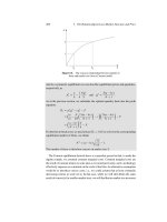
Figure 1.11 illustrates how much plant 1 would have to increase its plant size to
achieve the MES. In that particular example, long-run costs increase beyond the
MES. Even though MES is measured relative to a “long-run” cost measure, it is
important to note that the “long run” in this construction refers to a firm’s or plant’s
ability to change input levels holding all else equal. As a result, this intellectual
construction is more helpful for an analyst when attempting to understand costs in a

cross section of firms or plants at a given point in time than as an aid to understanding
what will happen to costs in some distant time period. As we have already noted,
over time both input prices and technology will typically change substantially.
We say a cost function demonstrates economies of scale if the long-run average
cost decreases with output. A firm with a size lower than the MES will exhibit
economies of scale and will have an incentive to grow. Diseconomies of scale occur
when the long-run average variable cost increases with output.
In the short run, economies and diseconomies of scale will refer to the behavior
of average and marginal costs as output is increased for a given capacity or plant
size. Mathematically, define
S D
AC
MC
D
C
Q@C=@Q
D
1
@ ln C=@ln Q
:
Thus we can derive a measure of the nature of economies of scale S directly from
an estimated cost function by calculating the elasticity of costs with respect to
1.2. Technological Determinants of Market Structure 29
AC, MC
q
i
MC
MES
LRAC
MES

MC
Plant 1
AC
Plant 1
AC
MES
Figure 1.11. The minimum efficient scale of a plant.
output and computing its inverse. Alternatively, one can also use S

D 1 MC=AC
as a measure of economies of scale, which obviously captures exactly the same
information about the cost function. If S>1, we have economies of scale because
AC is greater than MC. On the other hand, if S<1, we have diseconomies of scale.
There are many potential sources of economies of scale. First, it could be that one
of the inputs can only be acquired in large discrete quantities resulting in the firm
having lower unit costs as it uses all of this input. An example would be the purchase
of a passenger plane with several hundred available seats or the construction of an
electricity grid. Also, as size increases, there may be scope for a more efficient
allocation of resources within a firm resulting in cost savings. For example, small
firms might hire generalists good at doing lots of things while a larger firm might
hire more efficient, but indivisible, specialized personnel. Sources of economies of
scale can be numerous and a good knowledge of the industry will help uncover the
important ones.
If we have substantial economies of scale, the minimum efficient size of a firm
may be big relative to the size of a market and as a result there will be few active
firms in that market. In the most extreme case, to achieve efficiency a firm must be
so large that only one firm will be able to operate at an efficient scale in a market.
Such a situation is called a “natural” monopoly, because a benevolent social planner
would choose to produce all market output using just one firm. Breaking up such a
monopoly would have a negative effect on productive efficiency. Of course, since

breaking up such a firm may remove pricing power, we may gain in allocative
efficiency (lower prices) even though we may lose in productive efficiency (higher
costs).
30 1. The Determinants of Market Outcomes
1.2.2.4 Scale Economies in Multiproduct Production
Determining whether there are economies of scale in a multiproduct firm can be a
fairly similar exercise as for a single-product firm.
23
However, instead of looking at
the evolution of costs as output of one good increases, we must look at the evolution
of costs as the outputs of all goods increase. There are a variety of possible senses in
which output can increase but we will often mean “increase in the same proportion.”
In that case, the term “economies of scale” will capture the evolution of costs as the
scale of operation increases while maintaining a constant product mix.
Ray economies of scale (RES) occur when the average cost decreases with an
increase in the scale of operation, or, equivalently, if the marginal cost of increasing
the scale of operations lies below the average cost of total production.
In order to formalizeournotion of economies of scale ina multiproduct environment,
let us first define the multiproduct cost function, C.q
1
;q
2
/. Next fix two quantities
q
0
1
and q
0
2
and define a new function

Q
C.Q j q
0
1
;q
0
2
/ Á C.Qq
0
1
;Qq
0
2
/;
where Q is therefore a scalar measure of the scale of output which we will vary
while holding the proportion of the two goods produced fixed. Total production can
be expressed as
.q
1
;q
2
/ D Q

.q
0
1
;q
0
2
/:

Graphically, if we trace a ray through all the points (Qq
0
1
;Qq
0
2
), Q >0, our multi-
product measure of economies of scale will measure the economies of scale of the
cost function above the ray (see figure 1.12).
The slope of the cost function along the ray is called the directional derivative by
mathematicians, and provides the marginal cost of increasing the scale of operations:
e
MC.Q/ D
@
Q
C.Q/
@Q
D
@C.Qq
0
1
;Qq
0
2
/
@Q
D
@C.q
1
;q

2
/
@q
1
@q
1
@Q
C
@C.q
1
;q
2
/
@q
2
@q
2
@Q
D
2
X
iD1
MC
i
q
0
i
:
Given
RES D

f
AC
e
MC
D
Q
C .Q/=Q
e
MC.Q/
D
Â
@ ln
Q
C.Q/
@ ln Q
Ã
1
,
RES >1 implies that we have ray economies of scale,
RES <1 implies that we have ray diseconomies of scale.
23
For a very nice summary of cost concepts for multiproduct firms, see Bailey and Friedlander (1982).
1.2. Technological Determinants of Market Structure 31
1.2.2.5 Economies of Scope
Although economies of scale in multiproduct firms mirror the analysis of economies
and diseconomies of scale in the single-output environment, important features of
costs can also arise from the fact that several products are produced. The cost of
producing one good maydepend on the quantity produced oftheother goods. Indeed,
it may actually decreasebecauseof the production of these other goods.For example,
nickel and palladium are two metals sometimes found together in the ground. One

option would be to build separate mines for extracting the nickel and palladium, but
it would obviously be cheaper to build one and extract both from the ore.
24
Similarly,
if a firm provides banking services, the cost of providing insurance services might be
less for this firm than for a firm that only offers insurance. Such effects are referred
to as economies of scope. Economies of scope can arise because certain fixed costs
are common to both products and can be shared. For instance, once the reputation
embodied in a brand name has been built, it can be cheaper for a firm to launch other
successful products under that same brand.
Formally, economies of scopeoccur when it ischeaperto produce a given levelofout-
put of two products . Qq
1
; Qq
2
/ together compared with producing the two products sep-
arately by different firms (see Panzar and Willig 1981). To determine economies of
scope we want to compare C.Qq
1
; Qq
2
/ and C.Qq
1
;0/CC.0; Qq
2
/. If there are economies
of scope, we want to understand the ranges over which they occur. For instance, we
want to know the set of . Qq
1
; Qq

2
/ for which costs of joint production are lower than
individual production:
f. Qq
1
; Qq
2
/ j C.Qq
1
; Qq
2
/<C.Qq
1
;0/C C.0; Qq
2
/g:
In addition, we will say cost complementarities arise when the marginal cost of
production of good 1 is declining in the level of output of good 2:
@
@q
2
Â
@C.q
1
;q
2
/
@q
1
Ã

D
@
2
C.q
1
;q
2
/
@q
2
@q
1
<0:
An example of a cost function with economies of scope is the multiproduct func-
tion shown in figure 1.12. In the figure the cost of producing both goods is clearly
lower than the sum of the costs of producing both goods separately. In fact, the
figure shows there is actually a “dip” so that the cost of producing the two goods
together is lower than the cost of producing them each individually. Clearly, this
cost function demonstrates very strong form of economies of scope.
25
24
For example, the Norilsk mining center in the Russian high arctic produces nickel, palladium, and
also copper. In that case, nickel mining began before the others at the surface, and underground mining
began later.
25
Note that it is sometimes important to be careful in distinguishing “economies of scope” from
“subadditivity” where a single-product cost function satisfies C.q
1
C q
2

/<C.q
1
C 0/ CC.0Cq
2
/.
32 1. The Determinants of Market Outcomes
Cost
q
1
C(0, q
1
)
C(0, q
2
)
C(q
1
, q
2
)
C(q
1
, 0)
q
2
(
q
1
, 0
)

(
q
1
,
q
2
)
C
ost functio
n
above ra
y
Ra
y
Ra
y
Cost
(
Q
; q
1
, q
2
) = C(Qq
1
, Qq
2
)
00 0 0
Figure 1.12. A multiproduct cost function. No unique notion of economies of scale in mul-

tiproduct environment, so we consider what happens to costs as expand production keeping
output of each good in proportion. Source: Authors’rendition of a multiproduct cost function
provided by Evans and Heckman (1984a,b) and Bailey and Friedlander (1982).
Economies of scope can have an effect on market structure because their existence
will promote the creation of efficient multiproduct firms. When considering whether
to break up or prohibit a multiproduct firm, it is in principle informative to examine
the likely existence or relevance of economies of scope. In theory, it should be easy to
evaluate economies of scope, but in practice when using estimated cost functions one
must be extremely careful in assessing whether the cost estimates should be used.
Very often one of the scenarios has never been observed in reality and therefore
the hypothesis used in constructing the cost estimates can be speculative and with
little possibility for empirical validation. A discussion of constructing cost data in a
multiproduct context is provided in OFT (2003).
26
In a multiproduct environment, conditional single-product cost functions tell us
what happenstocosts when theproduction of oneproduct expandswhilemaintaining
constant the output of other products. Graphically, the cost function of product 1
conditional on the output of product 2 is represented as a slice of the cost function
in figure 1.13 that, for example, is above the line between .0; q
2
/ and .q
1
;q
2
/.
27
Conditional cost functions are useful when defining the average incremental cost
(AIC) of increasing good 1 by an amount q
1
, holding output of good 2 constant.

This cost measure is commonly used to evaluate the cost of a firm’s expansion in a
particular line of products.
26
See, in particular, chapter 6, “Cost and revenue allocation,” as well as the case study examples in
part 2.
27
These objects are somewhat difficult to visualize in what is a complex graph. The central approach
is to consider the univariate cost functions that result when the appropriate “slice” of the multivariate
cost function is taken.
1.2. Technological Determinants of Market Structure 33
Cost
q
1
C(0, q
1
)
C(0, q
2
)
C(q
1
, q
2
)
q
2
(0, q
2
)
(q

1
, 0)
(q
1
, q
2
)
Usual single-product
cost function for q
1
, q
2
= 0
Cost function as
expand q with q fixed
C(q
1
, 0)
Figure 1.13. Conditional product cost function in multiproduct environment. We can still
consider what happens to costs as the firm expands production of a single output at any fixed
level of output of the other good.
Formally, the conditional average incremental cost function is defined as
AIC
1
.q
1
j q
2
/ D
C.q

1
C q
1
j q
2
/  C.q
1
j q
2
/
q
1
:
The conditional single-output marginal cost is defined as
MC
1
.q
1
j q
2
/ D
@C.q
1
;q
2
/
@q
1
:
Product-specific economies of scale can also be evaluated. Economies of scale in

product 1, holding output of product 2 constant, are defined as
S
1
.q
1
j q
2
/ D
AIC.q
1
j q
2
/
MC.q
1
j q
2
/
:
As usual, S
1
>1indicates the presence of economies of scale in the quantity
produced of good 1 conditional on the level of output of good 2, while S
1
<1
indicates the presence of diseconomies of scale.
1.2.2.6 Endogenous Economies of Scale
The discussion above has centered on economies of scale that are technologically
determined. We discussed inputs that were necessary to production and that entered
the production function in a way that was exogenously determined by the technol-

ogy. However, firms may sometimes enhance their profits by investing in brands,
advertising, and design or product innovation. The analysis of such effects involves
34 1. The Determinants of Market Outcomes
important demand-side elements but also has implications on the cost side. For
example, if R&D or advertising expenditures involve large fixed outlays that are
largely independent of the scale of production, they will result in economies of
scale. Since firms will choose their level of R&D and advertising, these are often
called “endogenous” fixed costs.
28
The decision to advertise or create a brand is
not imposed exogenously by technology but rather is an endogenous decision of
the firm in response to competitive conditions. The resulting economies of scale are
also endogenous and, because the consumer welfare contribution of such expen-
ditures may or may not be positive, it may or may not be appropriate to include
them with the technologically determined economies of scale in the assessment of
economies of scale and scope, depending on the context. For example, it would be
somewhat odd for a regulator to uncritically allow a regulated monopoly to charge
a price which covered any and all advertising expenditure, irrespective of whether
such advertising expenditure was in fact socially desirable.
1.2.3 Input Demand Functions
Input demand functions provide a third potential source of information about the
nature of technology in an industry. In this section we develop the relationship
between profit maximization and cost minimization and describe the way in which
knowledge of input demand equations can teach us about the nature of technology
and more specifically provide information about the shape of cost functions and
production functions.
1.2.3.1 The Profit-Maximization Problem
Generally, economists assume that firms maximize profits rather than minimize
costs per se. Of course, minimizing the costs of producing a given level of output
is a necessary but not generally a sufficient condition for profit maximization. A

profit-maximizing firm which is a price-taker on both its output and input markets
will choose inputs to solve
max
L;K;F
˘.L; K; F; p; p
L
;p
k
;p
F
;uI˛/
D max
L;K;F
pf.L;K;F;uI˛/  p
L
L  p
K
K  p
F
F; (1.1)
where L denotes labor, K capital, F a third input, say, fuel, and f.L;K;F;uI˛/ the
level of production; p denotes the price of the good produced and the other prices
.p
L
;p
K
;p
F
/ are the prices of the inputs. The variable u denotes an unobserved effi-
ciency component and ˛ represents the parameters of the firm’s production function.

28
Sutton (1991) studies the case of endogenous sunk costs. In his analysis, he assumes that R&D and
advertising expenditures are sunk by the time firms compete in prices although in other models they need
not be.
1.2. Technological Determinants of Market Structure 35
If the firm is a price-taker on its output and input markets, then we can equivalently
consider the firm as solving a two-step procedure. First, for any given level of output
it chooses its cost-minimizing combination of inputs that can feasibly supply that
output level. Second, it chooses how much output to supply to maximize profits.
Specifically,
C.Q;p
L
;p
K
;p
F
;uI˛/ D min
K;L;F
p
L
L C p
K
K C p
F
F
subject to Q 6 f.K;L;F;uI˛/ (1.2)
and then define
max
Q
˘.Q; p; p

L
;p
K
;p
F
;uI˛/ D max
Q
pQ  C.Q;p
L
;p
K
;p
F
;uI˛/: (1.3)
With price-taking firms, the solution to (1.1) will be identical to the solution of the
two-stage problem, solving (1.2) and then (1.3).
If the firm is not a price-taker on its output market, the price of the final good p
will depend on the level of output Q and we will write it as a function of Q, P.Q/,in
the profit-maximization problem. Nonetheless, we will still be able to consider the
firm as solving a two-step problem provided once again that the firm is a price-taker
on its input markets. Profit-maximizing decisions in environments where firms may
be able to exercise market power will be considered when we discuss oligopolistic
competition in section 1.3.
29
1.2.3.2 Input Demand Functions
Solving the cost-minimization problem
C.Q;p
L
;p
K

;p
F
;uI˛/ D min
K;L;F
p
L
L C p
K
K C p
F
F
subject to Q 6 f.K;L;F;uI˛/
29
If the firm is not a price-taker on its input markets, the price of the inputs may also depend on the
level of inputs chosen and, while we can easily define the firm’s cost function as
C.Q; uI ˛;#
L
;#
K
;#
F
/ D min
K;L;F
p
L
.LI #
L
/L C p
K
.KI #

K
/K C p
F
.F I #
F
/F
subject to Q 6 f.K;L;F;uI˛/;
the resulting cost function should not, for example, depend on the realized values of the input prices
but rather on the structure of the input pricing functions, C.Q;uI ˛;#
L
;#
K
;#
F
/. This observation
suggests that estimation of cost functions in environments where firms can get volume discounts from
their suppliers are certainly possible, but doing so requires both careful thought about the variables that
should be included and also careful thought about interpretation of the results. In particular, in general the
shape of the cost function will now capture a complex mixture of incentives generated by (i) substitution
possibilities generated by the production function and (ii) of the pricing structures faced in input markets.
36 1. The Determinants of Market Outcomes
produces the conditional input demand equations, which express the inputs
demanded as a function of input prices, conditional on output level Q:
L D L.Q; p
L
;p
K
;p
F
;uI˛/;

K D K.Q; p
L
;p
K
;p
F
;uI˛/;
F D F.Q;p
L
;p
K
;p
F
;uI˛/:
Conveniently, Shephard’s lemma establishes that cost minimization implies that the
inputs demanded are equal to the derivative of the cost function with respect to the
price of the input:
L D L.Q; p
L
;p
K
;p
F
;uI˛/ D
@C.Q; p
L
;p
K
;p
F

;uI˛/
@p
L
;
K D K.Q; p
L
;p
K
;p
F
;uI˛/ D
@C.Q; p
L
;p
K
;p
F
;uI˛/
@p
K
;
F D F.Q;p
L
;p
K
;p
F
;uI˛/ D
@C.Q; p
L

;p
K
;p
F
;uI˛/
@p
F
:
The practical relevance of Shephard’s lemma is that it means that many of the
parameters in the cost function can be retrieved from the input demand equations
and vice versa. That means we have a third type of data set, data on input demands,
that will potentially allow us to learn about technology parameters.
30
Finally, if firms are price-takers on output markets, solving the profit-maximizing
problem produces the unconditional input demand equations that express input
demand as a function of the price of the final good and the prices of the inputs:
L D L.p; p
L
;p
K
;p
F
;uI˛/;
K D K.p; p
L
;p
K
;p
F
;uI˛/;

F D F.p;p
L
;p
K
;p
F
;uI˛/:
Note that both conditional(onQ) and unconditional factor demand functions depend
on productivity, u. Firmswitha higher productivitywilltend to producemorebut will
use fewer inputs than other firms in order to produce any given level of output. That
observation has a number of important implications for the econometric analysis
of production functions since it can mean input demands will be correlated with
the unobservable productivity, so that we need to address the endogeneity of input
30
For a technical discussion of the result, see the section “Duality: a mathematical introduction”
in Mas-Colell et al. (1995). In the terminology of duality theory, the cost function plays the role of
the “support function” of a convex set. Specifically, let the convex set be S Df.K;L;F/ j Q 6
f.K;L;F;uI ˛/g and define the “support function” .p
L
;p
K
;p
F
/ D min
.K;L;F /
fp
L
L C
p
K

K C p
F
F j .L;K;F/ 2 Sg, then roughly the duality theorem says that there is a unique
set of inputs .L

;K

;F

/ so that p
L
L

C p
K
K

C p
F
F

D .p
L
;p
K
;p
F
/ if and only
if .p
L

;p
K
;p
F
/ is differentiable at .p
L
;p
K
;p
F
/. Moreover, L

D @.p
L
;p
K
;p
F
/=@p
L
,
K

D @.p
L
;p
K
;p
F
/=@p

K
, and F

D @.p
L
;p
K
;p
F
/=@p
F
.
1.3. Competitive Environments 37
demands in the estimation of production functions (see, for example, the discussion
in Olley and Pakes 1996; Levinsohn and Petrin 2003; Ackerberg et al. 2005). The
estimation of cost functions is discussed in more detail in chapter 3.
1.3 Competitive Environments: Perfect Competition, Oligopoly, and
Monopoly
In a perfectly competitive environment, market prices and output are determined by
the interaction of demand and supply curves, where the supply curve is determined
by the firms’ costs. In a perfectly competitive environment, there are no strategic
decisions to make. Firms spend their time considering market conditions, but do
not focus on analyzing how rivals will respond if they take particular decisions. In
more general settings, firms will be sensitive to competitors’ decisions regarding
key strategic variables. Both the dimensions of strategic behavior and the nature of
the strategic interaction will then be fundamental determinants of market outcomes.
In other words, the strategic variables—perhaps advertising, prices, quantity, or
product quality—and the specific way firms in the industry react to decisions made
by rival firms in the industry will determine the market outcomes we observe. The
primary lesson of game theory for firms is that they should spend as much time

thinking about their rivals as they spend thinking about their own preferences and
decisions. Whenfirmsdothat, we say that they are interacting strategically. Evidence
for strategic interaction is often quite easy to find in corporate strategy and pricing
documents.
In this section, we describe the basic models of competition commonly used to
model firm behavior in antitrust and merger analysis, where strategic interaction
is the norm rather than the exception. Of course, since this is primarily a text on
empirical methods, we certainly will not be able to present anything like a compre-
hensive treatment of oligopoly theory. Rather, we focus attention on the fundamental
models of competitive interaction, the models which remain firmly at the core of
most empirical analysis in industrial organization. Our ability to do so and yet cover
much of the empirical work used in practical settings suggests the scope of work
yet to be done in turning more advanced theoretical models into tools that can, as a
practical matter, be used with real world data.
While some of the models studied in this section may to some eyes appear highly
specialized, we will see that the general principles of building game theoretic eco-
nomic (and subsequently econometric) models are entirely generic. In particular,
we will always wish to (1) describe the primitives of the model, in this case the
nature of demand and the firms’ cost structures, (2) describe the strategic variables,
(3) describe the behavioral assumptions we make about the agents playing the game,
generally profit maximization, and then, finally, (4) describe the nature of equilib-
rium, generally Nash equilibrium whereby each player does the best they can given
38 1. The Determinants of Market Outcomes
the choice of their rival(s). We must describe the nature of equilibrium as each firm
has its own objective and these often competing objectives must be reconciled if a
model is to generate a prediction about the world.
1.3.1 Quantity-Setting Competition
The first class of models we review are those in which firms choose their optimal
level of output while considering how their choices will affect the output decisions
of their rivals. The strategic variable in this model is quantity, hence the name:

quantity-setting competition. We will review the general model and then relate its
predictions to the predicted outcomes under perfect competition and monopoly.
1.3.1.1 The Cournot Game
The modern models of quantity-setting competition are based on that developed
by Antoine Augustin Cournot in 1838. The Cournot game assumes that the only
strategic variable chosen by firms is their output level. The most standard analysis
of the game considers thesituationin which firms move simultaneously and thegame
has only one period. Also, it is assumed that the good produced is homogeneous,
which means that consumers can perfectly substitute goods from the different firms
and implies that there can only be one price for all the goods in the market. To aid
exposition we first develop a simple numerical example and then provide a more
general treatment.
For simplicity suppose there are only two firms and that total and marginal costs
are zero. Suppose also that the inverse demand function is of the form
P.q
1
C q
2
/ D 1  .q
1
C q
2
/;
where the fact that market price depends only on the sum of the output of the two
firms captures the perfect substitutability of the two goods. As in all economic
models, we must be explicit about the behavioral assumptions of the firms being
considered. A probably reasonable, if sometimes approximate, assumption about
most firms is that they attempt to maximize profits to the best of their abilities. We
shall follow the profession in adopting profit maximization as a baseline behavioral
assumption.

31
The assumptions on the nature of consumer demand, together with
the assumption on costs, which here we shall assume for simplicity involve zero
31
Economists quiterightly questionthe realityof thisassumption ona regular basis. Most of the time we
fairly quickly receive reassurance from firm behavior, company documents, and indeed stated objectives,
at least those stated to shareholders or behind closed doors. Public reassurances and marketing messages
are, of course, a different matter and moreover individual CEOs or other board members (and indeed
investors) certainly can consider public image or other social impacts of economic activity. For these
reasons and others there arealways departuresfrom at leasta narrow definitionof profit maximization and
we certainlyshould not bedogmatic aboutany ofour assumptions.And yetin terms ofits predictive power,
profit maximization appears to do rather well and it would be a very brave (and frankly irresponsible)
merger authority which approved, say, a merger to monopoly because the merging parties told us that
they did not maximize profits but rather consumer happiness.
1.3. Competitive Environments 39
m
q
2
Cournot–Nash equilibrium
1
1
0
q
1
q
1
m
q
2
(i)

(iii)
(ii)
(iv)
Figure 1.14. Reaction functions in the Cournot model. (i) R
1
.q
2
/W q
1
D
1
2
.1  q
2
/;
(ii) R
2
.q
1
/W q
2
D
1
2
.1  q
1
/; (iii) N
1
D q
1

.1  q
1
 q
2
/ (isoprofit line for firm 1);
(iv) N
2
D q
2
.1  q
1
 q
2
/ (isoprofit line for firm 2).
marginal costs, c
1
D c
2
D 0, allow us to describe the way in which each firm’s
profits depend on the two firms’ quantity choices. In our example,

1
.q
1
;q
2
/ D .P.q
1
C q
2

/  c
1
/q
1
D .1  q
1
 q
2
/q
1
;

2
.q
1
;q
2
/ D .P.q
1
C q
2
/  c
2
/q
2
D .1  q
1
 q
2
/q

2
:
Given our behavioral assumption, we can define the reaction function, or best
response function. This function describes the firm’s optimal quantity decision for
each value of the competitor’s quantity choice. The reaction function can be eas-
ily calculated given our assumption of profit-maximizing behavior. The first-order
condition from profit maximization by firm 1 is
@
1
.q
1
;q
2
/
@q
1
D .1  q
2
/  2q
1
D 0:
Solving for the quantity of firm 1 produces firm 1’s reaction function
q
1
D R
1
.q
2
/ D
1

2
.1  q
2
/:
If both firms choose their quantity simultaneously, the outcome is aNashequilibrium
in which each firm chooses their optimal quantity in response to the other firm’s
choice. The reaction functions of firms 1 and 2 respectively are
R
1
.q
2
/W q
1
D
1
2
.1  q
2
/ and R
2
.q
1
/W q
2
D
1
2
.1  q
1
/:

Solving these two linear equations describes the Cournot–Nash equilibrium
q
1
D
1
2
.1  q
2
/ D
1
2
.1 
1
2
.1  q
1
// D
1
2
.
1
2
C
1
2
q
1
/ D
1
4

C
1
4
q
1
;
so that the equilibrium output for firm 1 is
3
4
q
NE
1
D
1
4
H) q
NE
1
D
1
3
:
40 1. The Determinants of Market Outcomes
The equilibrium output for firm 2 will then be
q
NE
2
D
1
2

.1 
1
3
/ D
1
3
:
The resulting profits will be

NE
1
D 
NE
2
D
1
3
.1 
1
3

1
3
/ D
1
9
:
Graphically,theCournot–Nash equilibrium is theintersection between the two firms’
reaction curves as shown in figure 1.14.
The reaction function is the quantity choice that maximizes the firm’s prof-

its for each given quantity choice of its competitor. The profits for the different
combinations of output choices in a Cournot duopoly are plotted in figure 1.15.
Isoprofit lines show all quantity pairs .q
1
;q
2
/ that generate any given fixed level
of profits for firm 1. These lines would be represented by horizontal slices of the
surface in figure 1.15. We can define a given fixed level of profit N
1
as
N
1
D .1  q
1
 q
2
/q
1
:
Note that given a level of profits and quantity chosen by firm 1, the output of firm 2
can be inferred as
q
2
D 1  q
1

N
1
q

1
:
Isoprofit lines can be drawn in a contour plot as shown in figure 1.16. Firm 1’s
best response to any given q
2
is where it reaches highest isoprofit contour. The
figure reveals an important characteristic of the model: for a fixed output of firm 1,
firm 1’s profits increase as firm 2 lowers its output. If the competitor chooses not
to produce, the profit-maximizing response is to produce the monopoly output and
make monopoly profits. That is, if q
2
D 0, then q
1
D
1
2
.1  q
2
/ D 0:5 and the
profit will be
N
1
D .1  q
1
 q
2
/q
1
D .1  0:5  0/0:5 D 0:25:
More generally, the first-order conditions in the Cournot game produce the famil-

iar condition that marginal revenue is equated to marginal costs. Given the profit
function

i
.q
i
;q
j
/ D P.q
1
C q
2
/q
i
 C
i
.q
i
/;
the first-order conditions are
@
i
.q
1
;q
2
/
@q
i
D P.q

1
C q
2
/ C q
i
P
0
.q
1
C q
2
/
„
ƒ‚ …
Marginal revenue
 C
0
i
.q
i
/
„
ƒ‚…
Marginal cost
D 0;
which in general defines an implicit function we shall call firm i’s reaction curve,
q
i
D R
i

.q
i
/, where q
i
denotes the output level of the other firm(s).
32
In our
32
That is, we can think of the first-order condition defining a value of q
i
which, given the quantities
chosen by other firms, will set the first-order condition to zero.
1.3. Competitive Environments 41
1
0.75
0.50
0.25
0
0.75
0.50
0.
25
0.25
0.20
0.15
0.10
0.05
q
2
q

1
(i)
(iii)
(ii)
1
π
Figure 1.15. Profit function for a two-player Cournot game as a function of the strategic
variables for each firm. (i) For each fixed q
2
, firm 1 chooses q
1
to maximize her profits;
(ii) the q
1
that generates the maximal level of profit for fixed value of q
2
is firm 1’s best
response to q
2
; (iii) profits if firm 1 is a monopoly: q
2
D 0, q
1
D 0:5, ˘
1
D 0:25.
1.00.80.60.40.2
0.8
0.6
0.4

0.2
0
= 0.001
monopoly
R
1
(q
2
)
q
1
1
π
1
π
1
π
= 0.1
= 0.2
q
2
q
1
Figure 1.16. Isoprofit lines in simple Cournot model.
two-player case, we have two first-order conditions to solve, which can each in turn
be used to define the reaction functions q
1
D R
1
.q

2
/ and q
2
D R
2
.q
1
/. In general,
with N active firms we will have N first-order conditions to solve. Nash equilibrium
is the intersection of the reaction functions so that solving the reaction functions can
42 1. The Determinants of Market Outcomes
involve solving N nonlinear equations. Our numerical example makes these equa-
tions linear (and hence easy to solve analytically) by assuming that inverse demand
curves are linear and marginal costs constant. In general, however, computers can
usually solve nonlinear systems of equations for us provided a solution exists.
33
Ideally, we would like a “unique” prediction about the world coming out of the
model and we will get one only if there is a unique solution to the set of first-order
conditions.
34
Note that since profits are always revenues minus costs, marginal profitability can
as always be described as marginal revenue minus marginal cost. At a maximum,
the first-order condition will be zero and hence we have the familiar result that profit
maximization requires that marginal revenue equals marginal cost.
To see the impact of strategic decision making, at this point it is worth taking a
moment to relate the Cournot optimality conditions, with perhaps the more familiar
results from perfect competition and monopoly.
1.3.1.2 Quantity Choices under Perfect Competition
In an environment with price-taking firms, the first-order condition from profit maxi-
mization leads to equating the marginal cost of the firm to the market price, provided,

of course, that there are no fixed costs so that we can ignore the sometimes important
constraint that profits must be nonnegative:

i
.q
i
/ D pq
i
 C
i
.q
i
/ H)
@
i
.q
i
/
@q
i
D p C
0
i
.q
i
/ D 0 H) p D C
0
i
.q
i

/:
Evidently, if the price is €1 and the marginal cost of producing one more unit is
€0.90, then my profits will increase if I expand production by that unit. Similarly,
if the price is €1 while the marginal cost of production of the last unit is €1.01,
my profits will increase if I do not produce that last unit. Repeating the calculation
makes clear that quantity will adjust until marginal cost equals marginal revenue,
which by assumption in this context is exactly equal to price.
Going further, since all firms face the same price, all firms will choose their
quantities in order to help price equal marginal cost so that C
0
i
.q
i
/ D C
0
j
.q
j
/ D p.
In particular, that means marginal costs are equalized across firms because all firms
face the same selling price.
Note that joint cost minimization also implies that the marginal costs are equated
across active firms. Consider what happens when we minimize the total cost of
producing any given level of total output:
min
q
1
;q
2
C

1
.q
1
/ C C
2
.q
2
/ subject to q
1
C q
2
D Q:
33
For the conditions required for existence of a solution to these nonlinear equations and hence for
Nash equilibrium, see Novshek (1985) and Amir (1996).
34
In general, a system of N nonlinear equations may have no solution, one solution, or many solu-
tions. In economic models the more commonly problematic situation arises when models have multiple
equilibria. We discuss the issue of multiple equilibria further in chapter 5.
1.3. Competitive Environments 43
In particular, note that such a problem yields the following first-order optimality
conditions,
C
0
1
.q
1
/ D C
0
2

.q
2
/ D ;
where  is the Lagrange multiplier in the constrained minimization exercise. Clearly,
minimizing the total costs for any given level of production will involve equalizing
marginal costs.
Intuitively, if we had firms producing at different marginal costs, the last unit
of output produced at the firm with higher marginal costs could have been more
efficiently produced by the firm with lower marginal costs. Perfect competition, and
in particular the price mechanism, acts to ensure that output is distributed across
firms in a way that ensures that all units in the market are as efficiently produced
as possible given the existing firms’ technologies. It is in this way that prices help
ensure productive efficiency.
In perfectly competitive markets, prices also act to ensure that the marginal cost
of output is also equal to its marginal benefit, so that we have allocative efficiency.
To see why, recall that the market demand curve describes the marginal value of
output to consumers at each level of quantity produced. At any given price, the last
unit of the good purchased will have a marginal value equal to the price. The supply
curve of the firm under perfect competition is the marginal cost for each level of
quantity since firms adjust output until p D MC.q/ in equilibrium. Therefore, when
price adjusts to ensure that aggregate supply is equal to aggregate demand, it ensures
that the marginal valuation of the last unit sold is equal to the marginal cost of its
production. In other words, the market produces the quantity such that the last unit is
valued by consumers as much as it costs to produce. It is this remarkable mechanism
that ensures that the market outcome under perfect competition is socially efficient.
1.3.1.3 Quantity Setting under Monopoly
In a monopoly, there is only one firm producing and therefore the market price will
be determined by this one firm when it chooses the total quantity to produce. As
usual, the firm’s profit function is


i
.q
i
/ D P.q
i
/q
i
 C
i
.q
i
/
and the corresponding first-order condition is
@
i
.q
i
/
@q
i
D P.q
i
/ C P
0
.q
i
/q
i
„ ƒ‚ …
Marginal revenue

 C
0
i
.q
i
/
„
ƒ‚…
Marginal cost
D 0:
Note that the first-order condition from monopoly profit maximization is a special
case of the first-order condition under Cournot where the quantity of the other firms
is set to zero. The monopolist, like any profit-maximizing firm in any of the scenarios
analyzed, chooses its quantity in order to set marginal revenue equal to marginal
cost.
44 1. The Determinants of Market Outcomes
P
D
P
0
P
1
c
(ii)
Q
0
Q
1
= Q
0

+ 1
(i)
Figure 1.17. Demand, revenue, and marginal revenue.
(i) Loss of revenue Q
0
P ! QP
0
.Q/. (ii) Increase of revenue P
1
.
Note that the slope of the inverse demand function P
0
.q
i
/ is negative. That means
that the marginal revenue generated by an extra unit sold is smaller than the marginal
valuation by the consumers as represented by the inverse demand curve P.q
i
/.
Graphically, the marginal revenue curve is below the inverse demand curve for a
monopolist. The reason for this is that the monopolist cannot generally lower the
price of only the last unit. Rather she is typically forced to lower the price for all
the units previously produced as well. Increasing the price therefore increases the
revenue for each product which continues to be sold at the higher price, but reduces
revenue to the extent that the number of units sold falls. Figure 1.17 illustrates the
marginal revenue when the monopolist increases its sales by one unit from Q
0
to
Q
1

. To sell Q
1
, the monopolist must reduce its selling price to P
1
, down from P
0
.
The marginal revenue associated with selling that extra unit is therefore
MR D P
1
Q
1
 P
0
Q
0
D P
1
.Q
1
 Q
0
/ C Q
0
.P
1
 P
0
/
D P

1
 1 C Q
0
P D P
1
C Q
0
P:
Under a profit-maximizing monopoly, marginal revenue of the last unit sold is
lower than the marginal valuation of consumers. As a result, the monopoly outcome
is not socially efficient. At the level of quantity produced, there are consumers
for whom the marginal value of an extra unit is greater than the marginal cost of
supplying it. Unfortunately, even though some consumers are willing to pay more
than the marginal cost of production, the monopolist prefers not to supply them to
avoid suffering from lower revenues from the customers who remain. The welfare
loss imposed by a monopoly market is illustrated in figure 1.18.
1.3.1.4 Comparing Monopoly and Perfect Competition to the Cournot Game
In all competition models, profit maximization implies that the firm will set marginal
revenue equal to marginal cost: MR D MC. Whereas in perfect competition, firms’
1.3. Competitive Environments 45
Deadweight loss from
monopoly pricing
P
D
P
E
c
Q
E
MR

MR = c
Q
Figure 1.18. Welfare loss from monopoly pricing compared with perfect competition.
marginal revenue is the market price, in a monopoly market the marginal revenue
will be determined by the monopolist’s choice of quantity. In a Cournot game, the
marginal revenue depends on the firm’s output decision as well as on the rivals’
output choices.
Specifically, in a Cournot game, we showed that the first-order condition from
profit maximization,
Max
q
i

i
.q
i
;q
j
/ D P.q
1
C q
2
/q
i
 C
i
.q
i
/;
is

@
1
.q
1
;q
2
/
@q
1
D P.q
1
C q
2
/ C q
1
P
0
.q
1
C q
2
/  C
0
1
.q
1
/ D 0:
As always, the firm equates marginal revenue to marginal cost. As in the monopolist
case, the marginal revenue is smaller than the marginal valuation by the consumer.
In particular, because of the negative slope of the demand curve, we have

MR
1
.q
1
;q
2
/ D P.q
1
C q
2
/ C q
1
P
0
.q
1
C q
2
/<P.q
1
C q
2
/:
Graphically, the marginal revenue curve is below the demand curve.
First notice that under Cournot, the effect of the decrease in price P
0
.q
1
Cq
2

/ is
only counted for the q
1
units produced by firm 1, while under monopoly the effect
is counted for the entire market output.
Second, under Cournot, the marginal revenue of each firm is affected by its output
decision and by the output decisions of competing firms, outputs which do affect
the equilibrium price. The result is a negative externality across firms. When firm 1
chooses its optimal quantity, it does not take into account the potential reduction in
profits that other firms suffer with an increase in total output. This effect is called
a “business stealing” effect. As a result Cournot firms will jointly produce and sell
46 1. The Determinants of Market Outcomes
m
q
2
Cournot–Nash equilibrium
1
1
0
q
1
q
1
m
q
2
(i)
(iii)
(ii)
(iv)

(v)
Figure 1.19. Cournot equilibrium versus monopoly: (i)–(iv) as in figure 1.14;
(v) output combinations that maximize joint profits.
at a lower price than an equivalent (multiplant) monopolist. Figure 1.19 illustrates
the joint industry profit-maximizing output combinations and the Cournot–Nash
equilibrium. If firms have the same constant marginal cost, any output allocation
among the two firms such that the sum of their output is the monopoly quantity, i.e.,
any combination fulfilling q
1
Cq
2
D Q
monopoly
, will maximize industry profits. The
industry profit-maximizing output levels are represented by the dashed line in the
figure. The Cournot–Nash equilibrium is reached by each firm maximizing its profits
individually. It is represented by the intersection of the two firms’ reaction function.
The total output in the Cournot–Nash equilibrium is larger than under monopoly. At
a very basic level, competition authorities which apply a consumer welfare standard
are aiming to maintain competition so that the negative externalities across firms
are preserved. In so doing they ensure that firms endow positive externalities on
consumers, in the form of consumer surplus.
Under perfect competition, social welfare is maximized because the market
equates the marginal valuations with the marginal cost of production. A monop-
olist firm will decide not to produce units that are valued more than their costs in
order not to decrease total profits and therefore social welfare is not maximized.
That said, production costs are still minimized.
35
Social welfare is not maximized
with Cournot competition but the loss of welfare is less severe than in the monopoly

game thanks to the extra output produced as a result of the Cournot externalities.
Output and social welfare will be higher than in the monopolist case since the firm
does not factor in the effect of lower prices on the other firms’ revenues. When
35
Experience suggests that monopolies will often, among other things, suffer from X-inefficiency as
well as restricting output, so this result should probably not be taken too literally. (See the literature on
X-inefficiency following Leibenstein (1966).)
1.3. Competitive Environments 47
a firm’s output expansion only has a small effect on price, the Cournot outcome
becomes close to the competitive outcome. This is the case when there are a large
number of firms and each firm is small relative to total market output. In a Cournot
equilibrium, marginal cost can vary across firms and so industry production costs
are not necessarily minimized unless firms are symmetric and marginal costs are
equal across firms.
In summary, Cournot equilibrium will be bad for the firms’ profits but good for
consumer welfare relative to the monopoly outcomes. On the other hand, Cournot
will be good for the firms’ profits but bad for consumer welfare relative to a market
with price-taking firms.
The Cournot model has had a profound impact on competition analysis and it is
sometimes described as the model that antitrust practitioner’s have in mind when
they first consider the economics of a given situation. As we discuss in chapter 6, the
model is, among other things, the motivation for considering the commonly used
Herfindahl–Hirschman index (HHI) of concentration.
1.3.2 Price-Setting Competition
Oligopoly theory was developed to explain what would happen in markets when
there were small numbers of competing firms. Cournot’s (1838) theory was based on
a form of competition in which firms choose quantities ofoutputandthe construction
appeared to fit with the empirical evidence that firms seemed to price above marginal
cost, the price prediction of the perfect competition model. While Cournot was suc-
cessful in predicting price above marginal cost, some unease remains about whether

firms genuinely choose the level of output they produce or determine their selling
price and sell whatever demand there is for the product at that price. This observation
motivated the analysis of what became one of the most important theoretical results
in oligopoly theory, Bertrand’s paradox.
1.3.2.1 The Bertrand Paradox
Bertrand (1883) considered that Cournot’s model embodied an unrealistic assump-
tion about firm behavior. He suggested that a more realistic model of actual firm
behavior was that firms choose prices and then supply the resulting demand for their
product. If so, then price rather than quantity would be the relevant strategic variable
for the firms. Bertrand’s model does indeed seem highly intuitive since firms do fre-
quently set prices for their products. Thus from the point of view of the description
of actual firm behavior, it seems to fit reality better than Cournot’s model. Nonethe-
less, we now treat Bertrand’s model as important because it produces paradoxical,
counterintuitive results.
36
Like many results in economics, Bertrand’s results are
36
A paradox is defined in the Oxford English Dictionary as a statement or tenet contrary to received
opinion orbelief; often with the implication that itis marvelous orincredible; sometimeswith unfavorable
connotation, as being discordant with what is held to be established truth, and hence absurd or fantastic.