Quantitative Techniques for Competition and Antitrust Analysis_11 pptx

478 9. Demand System Estimation
and cross-price elasticities. In practice, therefore, MNL models are quite good for
learning about the characteristics which tend to be associated with high or low levels
of market shares, but we recommend strongly against using MNL models in situa-
tions where we must learn about substitution patterns (e.g., for merger simulation).
There have been a number of responses to the problems the literature has identified
with MNL and we explore some of those responses in the rest of this section. The
important lesson from MNL and the property of independence of irrelevant alterna-
tives (IIA) is not that the MNL is a hopeless model (though that is probably true),
but rather that we can use the IIA property to our advantage; since the MNL makes
unreasonable predictions about what will happen to market shares following entry,
if we observe what happens to market shares following entry, we will be able to use
data to reject MNL models and identify parameters in richer discrete choice models.
Furthermore, the literature has grown from MNL models and many of its tools are
most simply explained in that context. For example, in the next section we explore
the introduction of unobserved product characteristics in the context of the MNL
models but we shall see later that the basic techniques for analyzing models with
unobserved product characteristics can be used in far richer discrete choice models.
9.2.4.3 Introducing Unobserved Product Characteristics in MNL Models
A famous, possibly true, marketing story is that the first car which introduced a
cupholder experienced dramatically high sales—customers thought it was a great
novel idea. Economists working with data from the time period, however, probably
would not have had a variable in their data set called “cupholder”—it would have
been a product characteristic driving sales, differentiating the product, which would
be observed by customers but unobserved by our analyst. Such a situation must
be common. As a result Bultez and Naert (1975), Nakanishi and Cooper (1974),
Berry (1994), and Berry et al. (1995) have each argued that we should introduce an
unobserved product characteristic into our econometric demand models. Following
Berry (1994), denote the unobserved product characteristic 
j
so that the conditional

indirect utility function that an individual gets from a given product j is
v
ij
DNv
j
C "
ij
D x
0
j
ˇ ˛p
j
C 
j
C "
ij
;
where x
j
is a vector of the observed product characteristics, 
j
is the unobserved
product characteristic (known to the consumer but not to the economist), and con-
sumer types are represented by "
i
D ."
i0
;"
i1
;:::;"

iJ
/. In general, there may be
many elements comprising 
j
but the class of models which have been developed
all aggregate unobserved product characteristics into one.
The parameters of the model which we must estimate are ˛ and ˇ. The basic
MNL model attempts to force observed product characteristics to explain all of
the variation in observed market shares, which they generally cannot. Instead of
9.2. Demand System Estimation: Discrete Choice Models 479
estimating a model
s
j
D s
j
.p;xI˛; ˇ/ C Error
j
;jD 0;:::;J;
where an error term is “tagged on” to each equation in the demand system, the new
model gives an explicit interpretation to the error term and integrates it fully into
the consumer’s behavioral model, s
j
D s
j
.p;x;I˛; ˇ/.
Of course, just introducing an unobserved product characteristic does not get you
very far. In particular, there is a clear potential problem with introducing unobserved
product characteristics in that the term enters in a nonlinear way—it is not obvious
how to run a regression in such cases. Fortunately, Nakanishi and Cooper (1974) and
Berry (1994) have shown that we can recover the unobserved product characteristics

from every product in the MNL model. Berry et al. (1995) then extend the “we can
recover the error terms” result to a far wider set of models.
To see how, define the vector of common (across individuals) utilities with the
common utility of the outside good normalized to zero Nv D .0; Nv
1
;:::; Nv
J
/. Suppose
we choose Nv to make the MNL model’s predicted market shares exactly match the
actual market shares so that
s
j
.p; Nv/ D s
j
for j D 1;:::;J:
Since Nv D .0; Nv
1
;:::; Nv
J
/,wehaveJ equations like the one specified above with
J unknowns. If the J equations match the predicted and actual market share of all
markets, then the market share of the outside good will also match s
0
.p;y; Nv/ D s
0
since the actual and predicted market shares must add to one.
40
Taking logs of the
market share equations gives us an equivalent system with J equations of the form:
ln s

j
.p
; Nv/ D ln s
j
for j D 1;:::;J;
where at a solution we will also have ln s
0
.p; Nv/ D ln s
0
. Recalling the normalization
condition Nv
0
D 0 so that expfNv
0
gD1, we can write
s
j
.p; Nv/ D
expfNv
j
g
1 C
P
K
kD1
expfNv
k
g
D s
0

.p; Nv/ expfNv
j
g;
so that
ln s
j
.p; Nv/ D ln s
0
.p; Nv/ CNv
j
for j D 1;:::;J:
40
In the continuous choice demand model context, we studied the constraint imposed by “adding up”:
that total expenditure shares must add to one. In a differentiated product demand system, we get a similar
“adding up” condition which enforces the condition that market shares add to one
J
X
j D0
s
j
D
J
X
j D0
s
j
.p;x;I ˛; ˇ/ D 1:
As a result of this condition we will, as before, be able to drop one equation from our analysis and study
the system of J equations. Generally, in the differentiated product context, the equation for the outside
good is dropped from the system of equations to be estimated.We impose the normalization that

v
0
D 0,
which in turn can be generated in part by the assumption that 
0
D 0.
480 9. Demand System Estimation
So that our J equations become
ln s
j
D ln s
0
.p; Nv/ CNv
j
for j D 1;:::;J:
At a solution we know that ln s
0
.p; Nv/ D ln s
0
so that we know a solution must have
the form
Nv
j
D ln s
j
 ln s
0
;
where the shares on the right-hand side are observed data. Thus the mean utilities
Nv D .0; Nv

1
;:::; Nv
J
/ that exactly solve the market share equations s
j
.p; Nv/ D s
j
are
just
Nv
j
D ln s
j
 ln s
0
for j D 1;:::;J;
where s
0
D 1 
P
J
kD1
s
k
. This formula states that, for the MNL model, we only
need information about the levels of market shares to figure out what the utility
levels of the models must be in order to rationalize those market shares. The mean
utility vector Nv is uniquely determined by the observed market shares. This allows
us to write and estimate the linear equation with now “observed” level of utility as
the dependent variable:

ln s
j
 ln s
0
D x
j
ˇ ˛p
j
C 
j
:
Note that this formulation of the model provides a simple linear-in-the-parameters
regression model to estimate, a familiar activity. The prices p
j
and product char-
acteristics x
j
are observed, the parameters to be estimated are ˛ and ˇ and the
error term is the unobserved product characteristic 
j
. Since this is a simple linear
equation we can use all of our familiar techniques upon it, including instrumental
variable techniques.
For the avoidance of doubt, note that the market shares in this equation are volume
market shares (or equivalently here number of purchasers, since in this model only
one inside good can be chosen per person). In addition, the market shares must be
calculated as a proportion of the total potential market S including the set of people
who choose the outside good. The appropriate way to calculate the total potential
market can be a matter of controversy, depending on the setting. In the new car
market it may be reasonable to assume that the largest potential market is for each

person of driving age to buy a new car. In breakfast cereals it may be reasonable to
assume that at most all people in the country will eat one portion of cereal a day,
so, for example, no one eats bacon and eggs for breakfast if the price of cereal is
sufficiently low and the quality sufficiently high. Obviously, such propositions are
not uncontroversial: some people own two cars and some people eat two bowls of
cereal a day. It may sometimes be possible to estimate the market size S , though
few academic articles have managed to. More frequently, it is a very good idea to
test the sensitivity of estimation results to whatever assumption has been made.
Table 9.5 presents results from Berry et al. (1995). Specifically, in the first column
they report an OLS estimation of the logit demand specification and in the second
9.2. Demand System Estimation: Discrete Choice Models 481
Table 9.5. Estimation of the demand for cars.
OLS logit IV logit OLS
Variable demand demand ln.price/ on w
Constant 10.068 9.273 1.882
(0.253) (0.493) (0.119)
HP/weight
a
0.121 1.965 0.520
(0.277) (0.909) (0.035)
Air 0.035 1.289 0.680
(0.073) (0.248) (0.019)
MP$
a
0.263 0.052 —
(0.043) (0.086) —
MPG
a
— — 0.471
— — (0.049)

Size 2.431 2.355 0.125
(0.125) (0.247) (0.063)
Trend — — 0.013
— — (0.002)
Price 0.089 0.216 —
(0.004) (0.123)
Number of inelastic 1,494 22 n.a.
demands (˙2 SEs) (1,429–1,617) (7–101)
R
2
0.387 n.a. 0.656
Notes: The standard errors are reported in parentheses.
a
The continuous product characteristics—horsepower/weight, size, and fuel efficiency (miles per dollar
or miles per gallon)—enter the demand equations in levels but enter the column 3 price regression in
natural logs.
Source: Table III from Berry et al. (1995).
Columns 1 and 2 report MNL demand estimates obtained using (1) OLS and (2) IV. Column 3 reports
a regression of the price of car j on the characteristics of car j , sometimes called a “hedonic” pricing
regression. If a market were perfectly competitive, then price would equal marginal cost and the final
regression would tell us about the determinants of cost in this market.
column the instrumental variable (IV) estimation. Note in particular that the move
from OLS to IV estimation moves the price coefficient downward. This is exactly
as we would expect if price were “endogenous”—if it is positively correlated with
the error term in the regression. Such a situation will arise when firms know more
about their product than we have data about and price the product accordingly. In
terms of our opening example, a car which introduces the feature of cupholder will
see high sales and the firm selling it may wish to increase its price to take advantage
of high or inelastic demand. If so, then the unobserved product characteristic (our
error term) and price will be correlated.

We have mentioned previously that the multinomial logit model, even with the
introduction of an unobserved product characteristic, imposes severe and unde-
sirable structure on own- and cross-price elasticities. To see that result, recall
482 9. Demand System Estimation
that
ln s
j
.p;x;/ DNv
j
.p;x;/  ln.s
0
.p;x;//
DNv
j
.p
j
;x
j
;
j
/  ln
Â
1 C
J
X
kD1
expfv
k
.p
k

;x
k
;
k
/g
Ã
;
where Nv
j
D x
j
ˇ ˛p
j
C 
j
. Differentiating, it follows that
@ ln s
j
.p
;x;/
@ ln p
k
D˛p
k
s
k
.p;x;/ D˛p
k
s
k

for j ¤ k;
@ ln s
j
.p;x;/
@ ln p
j
D˛p
j
.1  s
j
.p;x;// D˛p
j
.1  s
j
/;
where the latter equalities follow when we evaluate the elasticities at a point where
predicted and actual market shares match.
This means that all own- and cross-price elasticities between any pair of products
j and k are entirely determined by one parameter ˛, the market share of the good
whose price changed and also the price of that good. Most strikingly, substitution
patterns do notdepend on how good substitutesgoods j and k really are, for example,
whether they have similar product characteristics. Because of the inflexible and
unrealistic structure that the MNL model imposes on the preferences, they probably
should never be used in merger simulation exercises or in any other exercise where
the pattern of substitution plays a central role in informing decision makers about
appropriate policy.
Despite all of the comments above, the MNL model does remain tremendously
useful in allowing analysts a simple way of exploring which product characteristics
play an important role in determining the levels of market shares. However, it is
often the departures from the simple MNL model that are most informative. For

example, it can be informative to include rival characteristics in product j ’s payoff
since that may inform us when close rival products drive down each individual
product’s market share because each product cannibalizes the demand for the other.
Indeed, it is precisely such patterns in the data that richer models will use to generate
more realistic substitution patterns than those implied by models such as MNL with
IIA. The observation is useful generally, but it also provides the basis of the formal
specification tests for the MNL proposed by Hausman and McFadden (1984).
9.2.5 Extending the Multinomial Logit Model
In this section we follow the literature in extending the MNL model to allow for
additional dimensions of consumer heterogeneity. To illustrate the process, we bring
together the MNL model with the Hotelling model and also the vertical product
differentiation model.
9.2. Demand System Estimation: Discrete Choice Models 483
Specifically, suppose that the conditional indirect utility function can be defined as
v
j
.z
j
;L
j
;p
j
;
j
;
i
;L
i
;"
ij

/ D 
i
z
j
 tg.d.L
i
;L
j
//  ˛p
j
C 
j
C "
ij
;
where the term z
j
is a quality characteristic where all consumers agree that all
else equal more is better than less—a vertical source of product differentiation.
Additionally, products are available in different locations L
j
and depending on the
consumer’s location L
i
the travel cost may be small or large—a horizontal source
of product differentiation. Finally, we suppose that consumers have an intrinsic
preference for particular products as in the multinomial logit. The consumer type in
this model is  D ."
i0
;"

i1
;:::;"
iJ
;L
i
;
i
/, where "
ik
represents the idiosyncratic
preference of consumer i for product k, L
i
indicates the individual’s taste for the
horizontal product characteristic, and 
i
represents his or her willingness to pay for
the vertical product characteristic.
As usual, aggregate demand is simply the sum of individual demands,
x
j
.z;L;p;I
i
;L
i
;"
i0
;:::;"
iJ
/;
over the set of all consumer types. In the first instance, that sum involves a .J C3/-

dimensional integral involving (J C 1) dimensions for the epsilons plus 1 each for
the location and vertical tastes L
i
, 
i
. Thus aggregate demand is
D
j
.s;L;p;/
D
•
";L;
x
j
.z;L;p;I
i
;L
i
;"
i0
;:::;"
iJ
/f
";L;
.";L
i
;IÂ/d" dL
i
d
D

Z

Z
L
expfz
k
 tg.d.L
j
;L
i
//  ˛p
j
g
P
K
kD1
expfz
k
 tg.d.L
k
;L
i
//  ˛p
k
g
f
L;
.L
i
;/dL

i
d:
For any given L
i
, 
i
, the model is exactly an MNL model. Thus we can use the MNL
formula to perform the integration over the .J C 1/ dimensions of consumer het-
erogeneity arising from the epsilons. Doing so means that the resulting integration
problem becomes in this instance just two dimensional, which is a relatively straight-
forward activity that can be accomplished using numerical integration techniques
such as simulation.
41
Berry et al. (1995) show that even in this kind of context we canfollow an approach
similar to that taken to analyze the MNL model. We discuss their model below, but
before doing so we describe the nested logit specification, which is a less flexible
but more tractable alternative popular among some antitrust practitioners.
41
For an introductory discussion in this context, see Davis (2000). For computer programs and a good
technical discussion, see Press et al. (2007). For a classic text, see Silverman (1989). For the econometric
theory underlying estimation when using simulation estimators, see Pakes and Pollard (1989), McFadden
(1989), and Andrews (1994).
484 9. Demand System Estimation
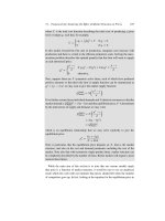
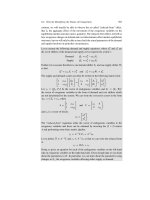
Rigids Tractors Outside good


Truck models Truck models
Figure 9.5. A model for the demand for trucks. Source: Ivaldi and Verboven (2005).
9.2.6 The Nested Multinomial Logit Model
The nested multinomial logit (NMNL) model is a somewhat more flexible structure

than the MNL model and yet retains its tractability.
42
It is based on the assumption
that consumers each choose a product in stages. The concept is very similar to the
nested model we studied by Hausman et al. (1994) for the demand for beer. In each
case, consumers first choose a broad category of products and then a specific product
within that category. Hausman et al. estimated their model using different regressions
for each stage. In contrast, the NMNL model allows us to estimate the demand for
the final products in a single estimation. Ivaldi and Verboven (2005) apply this
methodology in their analysis of a case from the European merger jurisdiction, the
proposed Volvo–Scania merger.
43
The product overlap of concern involved the sale
of trucks generally and heavy trucks in particular since the commission found that
heavy trucks constituted a relevant market. The authors suggest that the heavy trucks
market can be segmented into two groups involving (1) rigid trucks (“integrated”
trucks, from which no semi-trailer can be detached) and (2) tractor trucks, which
are detachable. A third group is specified for the outside good. Figure 9.5 describes
the nesting structure they adopt.
The NMNL model itself can be motivated in a number of ways.
Motivation method 1. McFadden (1978) initially motivated the NMNL model
by assuming that consumers undertook a two-stage decision-making process. At
the first stage he suggested they decide which broad category (group) of goods
g D 1;:::;Gto buy from and then, at the second stage, they choose between goods
within that group. Each of the groups consists of a set of products and all products
are in only one group. The groups are mutually exclusive and exhaustive collections
of products.
42
The link between consumer theory and discrete choice models is discussed in McFadden (1981) and
for the NMNL model, in particular, see also Verboven (1996).

43
Case no. COMP/M. 1672. Their exercise is described in chapter 8.
9.2. Demand System Estimation: Discrete Choice Models 485
Motivation method 2. Cardell (1997) (see also Berry 1994) provide an alternative
way to motivate the NMNL model as a random coefficient model with a conditional
indirect utility function defined as
v
ij
D
K
X
lD1
x
jl
ˇ
il
C 
j
C &
ig
C .1  /"
ij
for product j in group g;
v
i0
D &
i0
C .1  /"
i0
for the outside good;

where x
jl
is the lth observed product characteristics of product j , 
j
are the unob-
served product characteristics, &
ig
is the consumer preference for product group g,
and "
ij
is the idiosyncratic preference of the individual for product j . For reasons
we describe below, since for every individual any products in group g get the same
value of &
ig
, which in turn depends on , the parameter  introduces a correlation
in all consumers’tastes across products within a group. Consumers with a high taste
for group g, a large &
ig
, will tend to substitute for other products in that group
when the price of a good in group g goes up. The consumer type in a model with G
pre-specified groups is
Â
i
D .&
i1
;:::;&
iG
;"
i0
;"

i1
;:::;"
iJ
/:
Cardell (1997) showed that for given  ,if&
ig
are independent with "
ij
having a
type I extreme value distribution, then the expression &
ig
C.1/"
ij
will also have
a type I extreme value distribution if and only if &
ig
has a particular type I extreme
value distribution.
44
Cardell (1997) also showed that the required distribution of
&
ig
depends on the parameter  so that some authors prefer to write &
ig
./ and
&
ig
./ C .1  /"
ij
. The parameter  is restricted to be between zero and one. As

 approaches zero the model approaches the usual MNL model and the correlation
between goods in a given group becomes zero. On the other hand, as  increases
to one, so does the relative weight on &
ig
and hence correlation between tastes for
goods within a group.
Motivation method 3: the MEV class of models. A third way to motivate the
NMNL model is to consider it a special case of McFadden’s (1978) generalized
extreme-value (GEV) class of models (which is probably more appropriately called
the multivariate extreme-value (MEV) class of models since the statistics com-
munity use GEV to mean a generalization of the univariate extreme value distri-
bution). That model effectively relaxes the independence assumptions across the
tastes ."
i0
;:::;"
iJ
/ embodied in the MNL model. The basic bottom line is that the
MEV class of models assumes that the joint distribution of consumer types can be
expressed as
F."
i0
;:::;"
iJ
I/ D exp.H.e
"
i0
;:::;e
"
iJ
I//;

44
As Cardell describes, his result is analogous to the more familiar result that if "  N.0; 
2
1
/ and "
and v are independent, then " C v  N.0; 
2
1
C 
2
2
/ if and only if v  N.0; 
2
2
/.
486 9. Demand System Estimation
where H.r
0
;:::;r
J
I/ is a possibly parametric function (hence the inclusion of
parameters ) with some well-defined properties (e.g., homogeneity of some pos-
itive degree in the vector of arguments). We have already mentioned that the stan-
dard MNL model has distribution function F."
ij
/ D exp.e
"
ij
/ so that under
independence the multivariate distribution of consumer types is

F."
i0
;:::;"
iJ
I/ D F."
i0
/F ."
i1
/ F."
iJ
/
D exp
Â

J
X
j D0
e
"
ij
Ã
:
In that case the MNL corresponds to the simple summation function
H.r
0
;:::;r
J
I/ D
J
X

j D0
r
j
:
The “one-level” NMNL model developed by McFadden (1978) corresponds to a
choice of function
H.r
1
;:::;r
J
I/ D
G
X
gD1
Â
J
X
j 2=
g
r
1=.1/
j
Ã
1
;
where =
g
denotes the set of products placed into group g,  D , and the distribution
function is evaluated at r
j

D e
"
ij
. The outside good will often be put into its own
group. Davis (2006b) discusses this approach to understanding the discrete choice
literature and also proposes a new member of the MEV class of discrete choice
models which can be used to estimate discrete choice models which have far less
restrictive substitution patterns.
Whichever method is used to motivate the NMNL model, specifying the groups
appropriately is absolutely vital for the results one will obtain. The groups must be
specified before proceeding to estimate the model, and the choice of groups will have
implications for which goods the model predicts will be better substitutes for one
another. Recall that the parameter  controls the correlation in tastes between goods
within a group. Company information on market segments or consumer surveys
may be helpful in establishing which products are likely to be “closer” substitutes
and therefore form distinct market segments that can be associated with a particular
group.
Following the earlier literature, Berry (1994) shows that in a manner very similar
to that used for the MNL model the NMNL model can also be estimated using a
regression equation linear in the parameters that can be estimated with instrumental
variables (see Bultez and Naert 1975; Nakanishi and Cooper 1974). In particular,
we have
ln s
j
 ln s
0
D
K
X
lD1

x
jl
ˇ
l
C  ln s
j jg
C 
j
;
9.2. Demand System Estimation: Discrete Choice Models 487
where s
j jg
is the market share of product j among those purchased in group g.If
q
j
denotes the volume of sales of product j , then s
j jg
D q
j
=
P
j 2=
g
q
j
. The use of
instrumental variables is likely to be essential when using this regression equation
since there will be a clear correlation between the error term 
j
and the conditional

market shares s
j jg
. Verboven and Brenkers (2006) suggest allowing the parameter
of the model controlling the within-group taste correlation to be group-specific so
that
H.r
1
;:::;r
J
I/ D
G
X
gD1
Â
J
X
j 2=
g
r
1=.1
g
/
j
Ã
1
g
:
In that case, they show that Berry’s regression can be estimated similarly by
estimating G group-specific taste parameters,
ln s

j
 ln s
0
D
K
X
lD1
x
jl
ˇ
l
C 
g
ln s
j jg
C 
j
:
The additional taste parameters will help free-up substitution patterns across goods
within each group since they are no longer constrained to be the same across
groups. However, even this model will suffer from similar problems as MNL when
examining substitution across groups.
9.2.7 Random Coefficient Models
Economists studying discrete choice demand systems have used consumer hetero-
geneity to generate models with better properties than either pure MNL or even
NMNL models. These approaches have been taken with both aggregate data and
also consumer-level data. We focus primarily on approaches with aggregate-level
data but note that the models are identical, although their method of estimation typi-
cally is not.
45

In the aggregate demand literature, the first random coefficient models
were estimated by Boyd and Mellman (1980) and Cardell and Dunbar (1980) using
data from the U.S. car industry. Those authors did not incorporate an unobserved
product characteristic into their model. The modern variant of the random coeffi-
cient model for aggregate data was developed in Berry et al. (1995) and through
their initials (Berry, Levinsohn, and Pakes) is often referred to as the “BLP” model.
In principle, random coefficients can provide us with very flexible models that put
few constraints on the substitution patterns in demand. If the models place few con-
straints on substitution patterns, then in an ideal world with enough data we will be
able to use that data to learn about the true substitution patterns.
Because the utility is expressed in terms of product characteristics and not in
terms of products, the number of parameters to be estimated does not increase
exponentially with the number of products in the market as in the case of the AIDS
45
See Davis (2000) and the references therein for more on the connections between the two types of
discrete choice models.
488 9. Demand System Estimation
model. It is richer but also substantially harder to program and compute than either
the AIDS or the nested logit models.
The model allows for individual tastes for product characteristics. Following
BLP, suppose the individuals’ conditional indirect utility functions are expressed
as follows:
v
ij
D
K
X
lD1
x
jl

ˇ
il
C ˛ ln.y
i
 p
j
/ C 
j
C "
ij
;v
i0
D "
i0
;
where as before the variable x
jl
represents the characteristic l of product j .For
example, a product characteristic might be horsepower in the case of a car. The
coefficient ˇ
il
is the taste parameter of individual i for characteristic l. There is a
product-specific unobserved product characteristic 
j
and there is the usual MNL
random component "
ij
capturing an individual’s idiosyncratic taste for a given prod-
uct. As in previous cases, the valuation of the outside good is assumed to consist
only of an individual random component.

In this model, the consumer’s type can be summarized by the vector of individual
specific taste parameters and the individual’s income:
.y
i
;ˇ
i1
;:::;ˇ
iK
;"
i0
;"
i1
;:::;"
iJ
/:
As always, in an aggregate data discrete choice demand model we have to make
an assumption about how these types are distributed across the population, and we
assume the MNL elements are independent of the other tastes:
f.y
i
;ˇ
i1
;:::;ˇ
iK
;"
i0
;"
i1
;:::;"
iJ

/
D f.ˇ
i1
;:::;ˇ
iK
j y
i
/f .y
i
/f ."
i0
;"
i1
;:::;"
iJ
/:
Furthermore, BLP assume the distribution of the individual idiosyncratic terms
f."
i0
;"
i1
;:::;"
iJ
/ is made up of independent standard type I extreme value terms
(i.e., the multinomial logit assumption). For f.y
i
/, one can use the empirical distri-
bution of income, perhaps observed from survey data. One needs only to assume a
distribution for the random taste coefficients. The taste parameters may or may not
be independent of income, f.ˇ

i1
;:::;ˇ
iK
j y
i
/. BLP assume they are while Nevo
(2000) allows the taste parameters to vary with consumer characteristics including
income.
As always, the market demands are just the aggregated individual demands. Let
Â
D .y; ˇ
1
;:::;ˇ
K
;"
0
;"
1
;:::;"
J
/;
the vector of 1 CK CJ C1 elements determining the consumer type. The demand
9.2. Demand System Estimation: Discrete Choice Models 489
for product j will be
D
j
.p;x;/
D S
Z
fÂjv

j
.Â:/>v
k
.Â:/ for all k¤j g
f
Â
.Â/ dÂ
D S
Z
fÂjv
j
.Â:/>v
k
.Â:/ for all k¤j g
f
"
."/f
.y;ˇ
1
;:::;ˇ
K
/
.y; ˇ
1
;:::;ˇ
K
/ d" dy dˇ
1
dˇ
K

D S
Z
y;ˇ
s
MNL
ij
.p;x
;Iy
i
;ˇ
1i
;:::;ˇ
iK
/f
ˇ jy
.ˇ
1
;:::;ˇ
K
j y/f
y
.y/ dˇ
1
dˇ
K
;
where we have imposed the independence assumption between the individual-
product taste random vector " and the individual’s income and tastes for characteris-
tics. We also assume the multinomial logit distribution for " allows us to express the
individual demand for product j given the individual’s tastes for characteristics and

income, which we have denoted s
MNL
ij
.p;x
;Iy
i
;ˇ
1i
;:::;ˇ
iK
/. Computing aggre-
gate demand then “only” requires the .K C1/-dimensional integral to be calculated
numerically. This is typically performed using simulation techniques.
46
In their paper, BLP assume that the tastes for characteristics f.ˇ
i1
;:::;ˇ
iK
/
are normally distributed in the population and independent of income. Let
.!
i1
;:::;!
iK
/ be a set of standard normal N.0; 1/ random variables. Define
N
ˇ
1
;:::;
N

ˇ
K
to be the mean consumer’s taste parameters. And define .
1
;:::;
K
/
as variance parameters in the distribution of tastes. Then we can write
ˇ
il
D
N
ˇ
l
C 
l
!
il
for l D 1;:::;K;
which implies that the distribution of tastes in the population is normal:
0
B
@
ˇ
1
:
:
:
ˇ
K

1
C
A
 N
0
B
@
0
B
@
N
ˇ
1
:
:
:
N
ˇ
K
1
C
A
;
0
B
@

2
1
00

0
:
:
:
0
00
2
K
1
C
A
1
C
A
:
Given these distributional assumptions for tastes, we can equivalently write the
random coefficient conditional indirect utilities by decomposing the individual taste
for a given characteristic into a component which depends on the individual taste
and one which does not. We get
v
ij
D
K
X
lD1
x
jl
N
ˇ
l

C 
j
C
K
X
lD1

l
x
jl
!
il
C ˛ ln.y
i
 p
j
/ C "
ij
;
where the first two terms do not contain individual-specific elements (they are con-
stant across individuals) while the last three terms do contain individual-specific
elements. For example, the third term involves expressions 
l
x
jl
!
il
which puts a
46
See Nevo (2000) and also, in particular, the appendix of Davis (2006a), which provides practical

notes on the econometrics including how to calculate standard errors.
490 9. Demand System Estimation
parameter from the distribution of tastes in the population (which is to be estimated)

l
on an interaction between product characteristic x
jl
and consumer taste for that
characteristic, !
il
.
The individual conditional indirect utility function can be rewritten as
v
ij
DNv
j
C 
ij
;
where
Nv
j
Á
J
X
j D1
x
jl
N
ˇ

l
C 
j
and 
ij
Á
K
X
lD1
x
jl

l
!
il
C ˛ ln.y
i
 p
j
/ C "
ij
:
As always, market demands are just the aggregate of individual demands which is,
in this case, an integral. In terms of market shares,
s
j
.p;x; Nv/ D
Z
y;ˇ
s

ij
. Nv
j
;y
i
;ˇ
1i
;:::;ˇ
iK
;:::/f.y;ˇ/dy dˇ
1
dˇ
K
;
where Nv
j
Á
P
J
j D1
x
jl
N
ˇ
l
C 
j
is common across individuals. The BLP paper
shows that for given values of the prices p
, observed product characteristics x,

and parameters .
1
;:::;
K
;˛/, the J nonlinear equations
s
j
. Nv; p;xI
1
;:::;
K
;˛/D s
j
;jD 1;:::;J;
can be considered as J equations in the J unknowns Nv
j
and furthermore that there
is a unique solution to these equations under fairly general conditions. Furthermore,
BLP provide a remarkably useful technique for calculating the solution to these
nonlinear equations rapidly. Specifically, they show that all we need to do is to pick
an initial guess, perhaps a vector of zeros, and then use the following very simple
iteration:
Nv
New guess
j
DNv
Old guess
j
C ln s
o

j
 ln s
j
.p;x; Nv
Old guess
/ for j D 1;:::;J;
where s
o
j
is the observed market share and s
j
.p;x; Nv
Old guess
/ is the predicted market
share at this iteration’s values of the variables.
The BLP technique means that for fixed values of a subset of the models’ param-
eters, namely .
1
;:::;
K
;˛/, we can solve for the J common components of the
conditional indirect utilities . Nv
1
;:::; Nv
J
/ and so we can run the instrumental variable
linear regression exactly as we did in the MNL case
Nv
j
D

K
X
lD1
x
jl
N
ˇ
l
C 
j
in order to estimate the remaining taste parameters
N
ˇ
1
;:::;
N
ˇ
K
and also evalu-
ate the error term 
j
. We will get different residuals from this regression for each
value of the taste distribution parameters .
1
;:::;
K
;˛/. Hence, we will write

j
.

1
;:::;
K
;˛/. These taste distribution parameters need to be estimated. BLP
9.3. Demand Estimation in Merger Analysis 491
Table 9.6. BLP model: estimated parameters of demand equations.
Demand-side Parameter Standard Parameter Standard
parameters Variable estimate error estimate error
Means (
N
ˇ) Constant 7.061 0.941 7.304 0.746
HP/weight 2.883 2.019 2.185 0.896
Air 1.521 0.891 0.579 0.632
MP$ 0.122 0.320 0.049 0.164
Size 3.460 0.610 2.604 0.285
Standard deviations (
ˇ
)
Constant 3.612 1.485 2.009 1.017
HP/weight 4.628 1.885 1.586 1.186
Air 1.818 1.695 1.215 1.149
MP$ 1.050 0.272 0.670 0.168
Size 2.056 0.585 1.510 0.297
Term on price (˛)ln.  / 43.501 6.427 23.710 4.079
Source: Table IV in Berry et al. (1995).
use the general method of moments (GMM), but one might initially simply choose
them by minimizing the sum of squared errors in the model:
47
min
.

1
;:::;
K
;˛/
K
X
lD1

j
.
1
;:::;
K
;˛/
2
:
BLP apply their method to estimate the demand for cars. Their estimation results
are shown in table 9.6 while the resulting own-characteristic elasticities of demand
are shown in table 9.7.
Their results
48
show the own-price elasticity of a Mazda 323 to be 6.4 at a price of
$5,049 while the own-price elasticity of a BMW 735i is 3.5 evaluated at the price of
$37,490. Overall, the results predict that markups will be much higher for high-end
BMWs and Lexuses than for low-end Mazdas and Fords.
9.3 Demand Estimation in Merger Analysis
The above introduction to the common models used for demand system estimation
has hopefully served at least to illustrate that estimating demands, although an
essential part ofmanyquantification exercises,is quite acomplex and even optimistic
task. An analyst is faced with a trade-off between imposing structure from the

model that may not fully reflect reality and developing a model that is flexible
47
For technical details on the econometrics, see also Berry et al. (2004).
48
Note that table 9.7 describes the value of the attribute for that car as the first entry in each cell in the
table and the elasticity with respect to the characteristic as the second entry in each cell in the table.
492 9. Demand System Estimation
Table 9.7. The own-characteristic elasticity of demand.
Value of attribute/price
Elasticity of demand with respect to:
‚
…„ ƒ
Model HP/weight Air MP$ Size Price
Mazda323 0.366 0.000 3.645 1.075 5.049
0.458 0.000 1.010 1.338 6.358
Sentra 0.391 0.000 3.645 1.092 5.661
0.440 0.000 0.905 1.194 6.528
Escort 0.401 0.000 4.022 1.116 5.663
0.449 0.000 1.132 1.176 6.031
Cavalier 0.385 0.000 3.142 1.179 5.797
0.423 0.000 0.524 1.360 6.433
Accord 0.457 0.000 3.016 1.255 9.292
0.282 0.000 0.126 0.873 4.798
Taurus 0.304 0.000 2.262 1.334 9.671
0.180 0.000 0.139 1.304 4.220
Century 0.387 1.000 2.890 1.312 10.138
0.326 0.701 0.077 1.123 6.755
Maxima 0.518 1.000 2.513 1.300 13.695
0.322 0.396 0.136 0.932 4.845
Legend 0.510 1.000 2.388 1.292 18.944

0.167 0.237 0.070 0.596 4.134
TownCar 0.373 1.000 2.136 1.720 21.412
0.089 0.211 0.122 0.883 4.320
Seville 0.517 1.000 2.011 1.374 24.353
0.092 0.116 0.053 0.416 3.973
LS400 0.665 1.000 2.262 1.410 27.544
0.073 0.037 0.007 0.149 3.085
BMW 735i 0.542 1.000 1.885 1.403 37.490
0.061 0.011 0.016 0.174 3.515
Notes: The value of the attribute or, in the case of the last column, price, is the top number and the
number below it is the elasticity of demand with respect to the attribute (or, in the last column, price).
Source: Table V in Berry et al. (1995).
but computationally complex (or at least difficult). If the simpler option is chosen,
perhaps because of lack of resources one must be extremely cautious and probably
treat the answers obtained as at most indicative. Using models which impose the
answer is not learning about the world, it is learning only about the property of
your model, and obviously we should not, for example, be making merger decisions
because of properties of econometric models.Although the use of the simpler models
such as NMNL and its variants may be appropriate in many cases, in some instances
estimating such an “off-the-shelf” model can be useless at best and in fact actively
misleading. As in any quantitative exercise, demand estimation must be undertaken
by knowledgeable economists and the assumptions and results must be confronted
9.3. Demand Estimation in Merger Analysis 493
with the facts of the case. As a rule of thumb, if all the documents and the industry
and consumer testimony in a case points in one direction while the econometric
results point in another, then treat the econometric results with extreme caution. It
may be that the econometrics is right and able to tell you more than the anecdotes
but it may also be that the econometric analysis is based on invalid assumptions, a
poor model specification, or the data are not good enough. In this section we point
out some practical issues relating to model specification and the data needed for

estimation.
49
9.3.1 Specification Issues
The purpose of demand estimation is often to retrieve price elasticities and to calcu-
late their effect on optimal pricing. In the merger context, for example, we usually
want to evaluate the impact of a change in ownership on pricing and we saw in chap-
ter 8 that the impact depends on the own- and cross-price elasticities at least between
the merging parties’ products. Demand estimation can be very useful, particularly if
other more straightforward sources such as company estimates are unavailable. For
example, sometimes companies choose to measure price sensitivity and run exper-
iments to evaluate particularly their own-price elasticity of demand. We discussed
one such marketing experiment in chapter 4, where we also discussed approaches to
measuring diversion ratios using survey data. Demand estimation is another tool in
the economists’ toolbox—but one that is sometimes easy to physically implement
and yet difficult to use well.
If demand estimation produces unrealistic demand elasticities, one must revise
the specification of the demand model. Assuming that the demand estimation is cor-
rectly specified and that proper instruments are being used, one must check for other
sources of error. It could be that the time frame used is incorrect so that quantity
variation is not being correctly matched to the appropriate price variation; contracts,
for example, can mean price variation occurs annually while you might have quar-
terly data. It could also be that other factors explaining variation in sales such as
promotions, advertising campaigns, rival product entry, or changes in tastes are not
being appropriately accounted for. Those simple checks should be undertaken first.
Ultimately, it may be that the model is misspecified, particularly if a lot of structural
assumptions on the shape of preferences have been imposed. In this case, other more
flexible demand specifications may be more appropriate. Always remember that our
aim is to write down an approximation to the data-generating process (DGP) and that
the DGP will incorporate both the underlying economic process and the sampling
process being used to physically generate the data that end up on your computer.

49
The discussion draws partly on Hosken et al. (2002).
494 9. Demand System Estimation
9.3.1.1 The Functional Specification of the Demand System
Merger simulation results are sensitive to the assumed demand specification and
this has been elegantly demonstrated in Crooke et al. (1999). In simulation exercises
evaluating mergers in differentiated markets with price competition, they found that
simulations based on a log-linear specification predicted price increases three times
larger than simulations using linear demands. Using AIDS models produced price
increases twice as big as the linear demand model and the logit model showed an
increase in price 50% higher than the linear demand model. These results reflect the
fact that the greater the curvature of the demand curve, the lower the price elasticity
of demand as prices increase (think about moving upward and leftward along an
inverse demand curve that is either steeply or shallowly curved) and the greater the
incentives to increase prices after a merger.
On the one hand, such sensitivity is theoretically a highly admirable feature of
merger simulation models: the predicted price increases for a given merger will
depend on the form of the demand curve, an important input to the model. On
the other hand, it can often be difficult to have an a priori idea of which demand
specification is more adequate, particularly if there have not been large historical
variations in prices. With enough data we will be able to tell which type of demand
curve best fits the data, but we do not always (or even often) have large enough data
sets to be able to perform such checking systematically.
50
One response is to consider running merger simulations using several demand
specifications in order to assess the robustness and sensitivity of the estimates.
Crooke et al.’s experience suggests that estimation using a log-linear or an AIDS
model is likely to produce higher-end estimates of price effects while linear spec-
ification will produce lower-end estimates. It is not uninteresting to examine the
bracket of outcomes generated by the different models. If the sensitivity to the model

specification is very large, the merger simulation exercise may not be informative.
9.3.1.2 Accuracy of the Estimate of Demand Elasticity
Using evidence presented in court in merger proceedings, Walker (2005) also illus-
trates that small changes in the demand elasticity estimates at current prices can have
significant effects on the results of merger simulations. Even variation within the
confidence interval of very precisely estimated coefficients can significantly alter
predicted price increases from mergers. One should therefore be wary when slight
changes within realistic ranges of the elasticity estimate produce sharp changes in
50
On some occasions it would be possible to nest the models and use statistical tests to examine which
is preferred by the data; for example, linear and log-linear models can be tested using the Box–Cox test.
On the other hand, models such as linear demands and AIDS may need to be tested against each other
using nonnested model tests.
9.3. Demand Estimation in Merger Analysis 495
predicted price increases. Best practice is to calculate measures of uncertainty for
the price increases, not just for the parameters of the model that generates them.
51
9.3.2 Data Issues
One of the factors that has contributed to the development of demand estimation is
the increase in the availability of data. In particular, access to scanner data at the retail
level has provided economists with invaluable databases to estimate the demand for
consumer goods. Nonetheless, case workers often face considerable difficulties and
in this section we discuss some of the issues that practitioners commonly face with
respect to data.
9.3.2.1 Availability
Obviously, in order to successfully estimate demand curves one must have suitable
data available. Before undertaking an involved econometric exercise, one must be as
sure as possible that the data necessary to construct a meaningful model are available.
The data available may determine the choice of specification since different models
have different data requirements, but this discretion in choosing demand functional

forms because of data constraints should not be abused. The models make different
assumptions which may or may not be valid. Rather, it makes more sense to choose
an appropriate class of models that are realistically feasible in the time-frame likely
to be available for analysis and to try to gather the necessary data early in the
investigation. This can be done by obtaining public data, by purchasing data from
third party suppliers, or in a competition agency by issuing data requests to the firms.
In some sectors such as consumer goods retail data are available through specialized
firms such as TNS, IRI, or AC Nielsen. In other sectors data will be more difficult to
obtain but authorities should not hesitate to press firms to provide their transaction
data, which are typically available in some form.
52
Ideally, the data collected—though not necessarily from the firm—must include a
set of instruments that will make possible the identification of the demand function.
These instruments can be cost shifters for single demand estimation or variables
51
This can be done simply by drawing values of the models’estimated parameters from their estimated
distribution; wetypically haveestimatedsome parameters
O
ˇ and VarŒ
O
ˇ. If we draw an appropriatelylarge
number, say 1,000, of values of the parameters from the normal distribution N.
O
ˇ;Va r Œ
O
ˇ/ and for each
value of those parameters calculate the predicted price from the merger coming from a merger simulation
model, then we will get a distribution of predicted prices. Taking the 2.5th and 97.5th percentiles of that
distribution will give us a 95% confidence interval for the price increase arising from the merger.
52

This need not be burdensome on the firms if the agency is willing to clean the data. Indeed, it may
even provide free data-cleaning services to the firm involved if the cleaned data is subsequently returned.
On the other hand, if extracting appropriate data is a major task which will distract the entire computer
expertise of a firm, then obviously it would be appropriate to carefully consider whether it was necessary
to proceed on this basis. Firms will sometimes have an incentive to keep data away from competition
agencies so such “it’s impossible” claims should not be taken at face value. It is often appropriate to
send a member of staff to talk to the “data person” at a company, although often an “offer” to do so will
overcome apparently significant hurdles.
496 9. Demand System Estimation
that determine each of the prices to be estimated without affecting the demand of
that product in the case of markets with several differentiated products. Hausman,
for example, suggested using prices from other markets while BLP suggested using
product characteristics of rival products. In some contexts firms appear to run price
promotions in a way that is unrelated to the level of demand and in those cases
we can use price variation from such experiments to identify the slope of demand
curves—we will be able to estimatedownward-sloping demandcurves. For example,
demand curves estimated using supermarket scanner data are usually found to slope
downward and display what appear to be sensible substitution patterns, albeit ones
that need to be very carefully considered in light of dynamic effects.
53
The reason
is that demand in a given store is often unrelated to the decision to run a price
promotion which may be a regional or national decision. Cost data are sometimes
available from firms, but are often burdensome on firms to collect in a form that
can be used, and moreover are often not available at a frequency which would be
genuinely useful; many attempts to obtain cost data from firms will generate data
sets where costs appear not to vary over time. On the other hand, in some instances
high-quality cost data are available and then they can be used as instruments.
9.3.2.2 Aggregation
An observation in aneconometric estimation is often an aggregate of many individual

transactions. For instance, one may aggregate purchases of a given good over a day,
a week, or a month. Also one may aggregate over stores, chains, or distribution
channels. Aggregation typically works better when it is done over homogeneous
elements. Aggregating over distribution channels will make sense if the purchases
in all channels are similar in that they are done by similar customers at similar prices.
If this is not the case, aggregating transactions in a supermarket with transactions
in a specialty store may produce a demand elasticity which does not reflect any
customer group’s actual elasticity. That said, if it is the aggregate elasticity that is
required, then it may make sense to work with aggregate data.
Aggregation over time may involve taking into account the periodicity at which
prices change since we are attempting to model the data-generating process. If
we aggregate to a greater length of time, then doing so can sometimes remove a
considerable amount of the useful price variation in a data set. On the other hand,
aggregation can sometimes reduce the effect of measurement error.
54
The possibility
53
Short-run elasticities of demand can be far greater than long-run elasticities of demand (or vice versa)
depending on the context. For the recent literature, see the overview by Hendel and Nevo (2004). For a
more technical dynamic model of consumer choice with inventories, see Hendel and Nevo (2006a,b). For
the earlier literature see an older applied econometrics textbook using partial adjustment models such as
Berndt (1991). The latter are often more informative as practical tools within a merger context.
54
Adding together two independent random measurement error terms will not reduce variance—
aggregation will add up the noise. On the other hand, averaging will reduce variance so that, for example,
aggregate market shares calculated using large numbers of individual demands will suffer from very little
sampling error.
9.3. Demand Estimation in Merger Analysis 497
of intertemporal allocation such as inventory accumulation may also be considered
in order to avoid overestimating the demand elasticity when there are temporary

reductions in prices such as sales or promotions. That said, in a practical context
it may be possible to simply avoid modeling complex detailed dynamics that are
irrelevant for the issues at hand by choosing the right time period for analysis.
Aggregating over different varieties of products or types of packaging can also
impact the results since a “generic” price is constructed for a “generic” bundle of
product. One could test the sensitivity of different price and quantity specifications
on the results to make sure that the latter are sufficiently robust to be meaningful,
though doing so is often a time-consuming exercise.
While there are many theoretical and real dangers in aggregation in practice, if
you are interested in an aggregate quantity you will at some point have to aggregate.
Thus the choice is often not whether to aggregate, but rather whether to model the
disaggregate data and then aggregate or alternatively to model the aggregate data
directly. Theoretically, the former is likely to be preferred, but in practice the latter
will often produce more reliable results at lower cost. The reason is simple, namely
that the analyst is focusing directly on the quantity of interest. Suppose, for example,
one is interested in understanding the aggregate demand for computers. An analyst
must decide whether it truly makes sense to attempt to model the dynamics for all
individual brands, or not.A disaggregated approach would involve modeling perhaps
hundreds of demand equations, necessarily imperfectly. In contrast, looking at the
aggregate data involves looking at one time series and hiding a lot of the variation
across brands. Working with aggregate data will involve imperfect price, volume,
and quality measures. However, the dominant features of the aggregate data will be
clear, and in the computer industry are likely to involve prices going down while
volumes and quality go up.
9.3.3 Retail and Wholesale Elasticities
Retail transaction data are more likely to be publicly available than wholesale data
so the demand elasticity at the retail level may be easier to calculate than the derived
demand elasticity faced by manufacturers. There are intrinsic differences between
retail and manufacturer level elasticities. In cases where we are interested in the
upstream market, the retail demand elasticity can be useful to know, since, for

example, highly elastic downstream customers will tend to make the retailer a highly
elastic demander of manufacturers products. However, an estimated retail demand
elasticity should not “replace” a serious consideration of the actual demand elasticity
faced by the manufacturer, if that ultimately is the object of interest.
At the end of the day the retailer and manufacturer are participants in a different
market from the one involving transactions between retailer and end-consumer.
Prices in upstream markets are often more complex than prices at retail. Long-term
relationships between manufacturers and retailers are not uncommon and contracts
498 9. Demand System Estimation
may simultaneously cover a broad range of goods. The resulting pricing schemes
are often nonlinear and may also incorporate rebates, de facto bundling, contracting
of shelf space, or promotional co-payments. Retailer’s demand can be stickier than
consumers’demand because of those contractual agreements for a given price range.
It can also be stickier because individuals who work with one another for a period
of time may simply like each other. On the other hand, manufacturers may face
very high demand elasticities, and such elasticities may be evidenced by experience
of large retailers deciding to drop the manufacturer’s products altogether from its
shelves after modest price increases. Service levels are often important to retailers
and so in upstream retail markets it may be appropriate to obtain data on service
levels (e.g., percentage of orders of the manufacturers product actually delivered by
week) as well as data on prices.
In the simplest theoretical context, the elasticity of the derived demand at the
wholesale level can be expressed in term of the demand elasticity faced by retailers.
To see how, consider a retailer who sets a pure uniform linear price by solving
max
p
.p w/D
R
.p/;
where p is the retail price, w the wholesale price of the good and therefore the cost

to the retailer, and R is the index indicating the demand is that faced by the retailer.
The solution to this problem will be a retail (downstream) pricing function p

.w/
so that, assuming a one-to-one technology, where one unit of the manufacturer’s
product is sold downstream as one unit of the retailer’s product, the manufacturer’s
demand can be written as D
M
.w/ D D
R
.p

.w//.
Following, for example, Verboven and Brenkers (2006), we may write
@ ln D
M
.w/
@ ln w
D w
@ ln D
R
.p

.w//
@w
D w
p
p
@ ln D
R

.p/
@p
@p

.w/
@w
or
"
w
D
w
p
 "
r
 .pass-through rate/ D "
r
 "
wr
;
where w=p is the ratio of the wholesale price over the retail price,
"
w
D
@ ln D
M
.w/
@ ln w
is the demand elasticity faced by the manufacturer,
"
r

D
@ ln D
R
.p/
@ ln p
is the demand elasticity faced by the retailer, and
"
wr
D
@ ln p

.w/
@ ln w
is the retailer’s price elasticity with respect to the wholesale price. Since the elasticity
of the retail price with respect to the wholesale price is likely to be less than one, this
9.4. Conclusions 499
equivalence implies that the elasticity of the derived demand for the manufacturer
will generally be lower in absolute terms than the retailer demand elasticity.
Some considerable progress has been made recently on modeling vertical chains
using both uniform and nonlinear pricing structures to describethe contracts between
retailers and manufacturers. See, in particular, the recent contributions by Verboven
and Brenkers (2006), Villas-Boas (2007a,b), and Bonnet et al. (2006). That said,
those of us working in competition agencies still face important challenges in mod-
eling using the kinds of data sets we do sometimes have, namely data from both
manufacturer and retailer. One important characteristic of such data is that it some-
times demonstrates surprisingly little variation over time, in particular, in prices
while volumes vary enormously over time. (We discuss vertical relationship further
in chapter 10.)
9.4 Conclusions
 Demand estimation is central to the empirical analysis of competition issues.

The reason is simply that a model of demand allows us to characterize the
revenues that firms will obtain from their products. In turn, revenue plays
an important role in determining firm profitability, firm conduct, and market
outcomes.
 In principle, estimating market demand functions for homogeneous products
is the easiest activity for an applied economist as there is only one demand
equation to estimateand it depends ononly one price variable (and any demand
shifters such as income). Still, one must be careful to understand the drivers
of variation in the observed data and doing so will involve understanding
consumer behavior in that market as well as any significant factors that affect
it.
 In addition to industry understanding, even in a homogeneous product market,
particular attention must be paid to the specification of the model and the data
variation that is allowing the demand curve to be identified. Most demand
estimation exercises will require us to use instrumental variable techniques
in order to achieve identification. Good instruments must explain variation in
price given the variation already explained by the included exogenous vari-
ables and also be uncorrelated with unobserved determinants of demand. In
demand estimation, suitable instruments will typically involve a determinant
of supply that has no role on the demand side. The reason is that shifts in the
supply (pricing) side of the market will identify (trace out) the demand curve.
 Linear or log-linear demand models provide simple specifications to take
to data since the models are each linear in the parameters to be estimated.
Naturally, either assumption involves placing strong restrictions on the way
500 9. Demand System Estimation
in which price elasticities of demand vary (or do not vary in the log-linear
case) along the demand curve.
 There are various ways of categorizing demand models. One is according to
the number of products, homogeneous or differentiated product. Another is by
the nature of the choice consumers make—either continuous quantity choices

or discrete (0,1) quantity choices. A third categorization is to consider those
models which specify preferences over products and those which specify
preferences in terms of product characteristics.
 Almost ideal demand systems (AIDS) provide one important example of a
continuous choice differentiated product demand model that provides a spec-
ification of preferences over products. The AIDS model is easy to estimate
and has some attractive properties as an aggregate demand model.
 When there are many products in the market, further restrictions on the param-
eters are often necessary to make the model estimable given the kinds of
databases usually available. One source of parameter restrictions is choice
theory. Restrictions that can be imposed include the Slutsky symmetry, homo-
geneity in prices and income, and additivity, whereby expenditure shares must
add to one. In doing so the analyst must keep in mind that Slutsky symmetry
does not necessarily hold in aggregate demand systems, even if the underlying
consumer demands are generated strictly by consumers satisfying the axioms
of choice theory. A second approach to reducing the number of parameters
to be estimated is to model demand as generated by a multistage budgeting
process where first consumers choose which market segment to buy from
and then choose the specific brand to buy within that market segment. Such
models impose structure on the matrix of own- and cross-price elasticities
and in doing so reduces the number of parameters to be estimated. These two
approaches are not mutually exclusive.
 A third approach to reducing the number of parameters is to assume that con-
sumers care about product characteristics rather than products themselves. In
product-characteristic models wetypically distinguish between horizontaland
vertical sources of product differentiation. Horizontal differentiation refers to
situations in which customers’ ranking of options are different. The Hotelling
model produces demand functions dependent on prices and the product char-
acteristics. The distribution of individual consumer types is either observed
(when it is based on location, for instance, and the decision is the choice of

store) or must be assumed. Vertical differentiation refers to situations where
consumers rank options equally (all agree that one is better than the other)
although they vary in how they value quality and hence trade-off quality and
price.
9.4. Conclusions 501
 Consumer preferences are commonly defined over product characteristics in
discrete choice demand models. The multinomial logit (MNL) model is a sim-
ple example of a discrete choice model. However, MNL is not directly useful
in many modeling exercises as its structure places unrealistic restrictions on
substitution patterns. For this reason it is not a recommended model when we
are trying to understand actual substitution patterns, although it can be useful
for understanding what data variation drives variation in the levels of market
shares.
 The nested multinomial logit (NMNL) model provides a discrete choice model
which allows subsets of goods to be “closer” substitutes within a group than
with those in other groups. In such models, following a price rise of a particular
product, individuals will tend to substitute to goods in the same group, by
which we will mean a market segment or category. This model provides
greater flexibility in preferences than MNL and is useful when the market
segments can be clearly identified, although it is important to note that the
substitution patterns remain highly restrictive.
 The random coefficient MNL model allows the model to predict a greater
variety of substitution patterns but at the same time is harder and hence more
costly to estimate than the NMNL or AIDS models. The BLP version of this
model has now been estimated on quite a large variety of occasions. The richer
model allows the data to drive predicted substitution patterns rather than the
model, but it is important to note that, in practice, some researchers have
found the model’s parameters quite difficult to identify on limited data sets.
In addition, more popular implementations of the model often inadvertently
impose some quite important restrictions on demand systems, in particular,

Slutsky symmetry. Nonetheless this class of random coefficient models is an
important step forward for many applications—at least compared with NMNL
and MNL models.
 We end this chapter with a plea to the practitioner. When estimating demand
systems with the aim of retrieving elasticities and predicting price increases,
perhaps following a merger, one must be confident that the specification and
data used are both adequate. Reality checks and sensitivity tests are very
important during the process of model specification and in casework it is gen-
erally important that where at all possible econometrics and model predictions
should be supported by other evidence in the investigation, particularly qual-
itative information, before decision makers are encouraged to draw strong
policy conclusions.
10
Quantitative Assessment of
Vertical Restraints and Integration
In previous chapters we have discussed estimation and identification of the main
determinants of market outcomes, in particular demand estimation, cost estimation,
and estimation of strategic choice equations such as pricing equations. We also dis-
cussed the effects of changes in market structure or in the form of competition on
firms’ prices and output, both using reduced- and structural-form equations. In this
chapter, we examine firms’ decisions relating to issues beyond just their own prices
and output. In particular, we look at the restraints that firms may sometimes impose
on their commercial customers downstream. We discuss when we can empirically
determine the motives and effects of such behavior on market outcomes and, specifi-
cally, final consumers. Our intention is not to define what constitutes anticompetitive
behavior, as that will vary by jurisdiction, but rather to discuss potential techniques
that may help evaluate types of conducts that are often subject to antitrust scrutiny.
Before beginning any analyst should be aware that the empirical assessment of
vertical restraints is generally considerably more difficult than analysis of at least
a straightforward single horizontal merger for at least three reasons. First, in order

to understand vertical restraints it is usually necessary to understand at least two
markets, the market upstream and the market downstream. Second, the economic
theoretical framework is less fully developed than models such as Bertrand pricing.
And third, the empirical analysis of such markets is not very accessible to basic
(i.e., academic) researchers since we are often seeking to understand the contractual
relationships between firms which, while often observed by competition authorities,
are often unobserved by the academic community. The consequence has been less
empirical research on these topics overall.
A formal quantitative analysis of the effect(s) of vertical restraints or integration is
therefore both a complex task and one where the set of tools available for empirical
analysis is modest. For that reason, vertical restraints are often tackled using quali-
tative arguments about the likelihood of foreclosure and consumer harm rather than
detailed quantitative analysis. There have, however, been some interesting attempts
at empirical estimation of the effect of vertical practices and vertical integration
and we explore many of them in this chapter. Moreover, since the trend in the legal