Earth Sciences Part 5 doc
Bạn đang xem bản rút gọn của tài liệu. Xem và tải ngay bản đầy đủ của tài liệu tại đây (9.9 MB, 40 trang )
Earth Sciences
150
The clinopyroxenes of the Khibiny massif, predominating in the majority of rocks, are
represented by diopside, hedenbergite, augite, aegirine-augite and aegirine (Yakovenchuk
et al., 2005; Yakovenchuk et al., 2008). Diopside is a rock-forming mineral of alkali-
ultrabasic rocks, alkali-feldspar trachytes, melteigite-urtite, metamorphosed to hornfels
volcanogenic-sedimentary rocks of basalt composition and their host foyaite.
Hedenbergite is observed in fenitized hornfels (after tuffite) where it together with
aegirine forms parallel-columnar coronas around fayalite inclusions in albite. Aegirine-
augite is the main mineral of all types of nepheline syenites (5–50 vol. %), foidolites (up to
90 vol. %), apatite-nepheline rocks, fenitized rocks of the massif frame and xenoliths of
volcanogenic-sedimentary rocks in foyaite. In foyaite of the outer and central parts of the
massif, it predominates among the other iron-magnesium-bearing silicates and quite often
occupies a position subordinated in relation to aegirine, alkaline amphiboles, and annite
in foyaite, lyavochorrite and rischorrite of the Main Ring zone. Aegirine is a ubiquitous
primary and/or secondary mineral forming marginal zones around diopside-aegirine-
augite crystals or separate needle-like crystals obviously formed later than the other
clinopyroxenes (Yakovenchuk et al., 2005).
Diagrams of a change in clinopyroxene composition (Fig. 14) along the A–B–C–D–E–F
profile (see Fig. 1) shows, above all, a different degree of rock differentiation in the Main
Ring in its rich (the Koashva deposit, the Е point) and poor ore (Mt. Marchenko Peak, the С
point) parts. As the Main Ring is approached in the area at Mt. Marchenko Peak, the
clinopyroxenes of foyaite feature increasing contents of Са, Mg and Fe
2+
at the expense of
Na and Fe
3+
, which proceeds on transition to rischorrite attaining the maximum in ijolite-
urtite. Quite opposite is the situation in the area of the Koashva deposit, where the
clinopyroxene of foyaite is represented by aegirine with traces of Са, Mg and Fe
2+
. However,
the concentrations of these elements increase on transition to rischorrite and foidolites, with
ijolite-urtite also containing clinopyroxenes of the diopside-hedenbergite series.
Fig. 14. Variation of clinopyroxene composition along the A-B-C-D-E-F profile.
Self-Organization of the Khibiny Alkaline Massif (Kola Peninsula, Russia)
151
Diagram of the change of the Mg and Fe
2+
ratio in clinopyroxene composition demonstrates
consecutive increasing of the hedenbergite constituent from the border of the massif to the
Main Ring, where all rocks contain clinopyroxene with a maximal content of Fe
2+
, followed
by an abrupt decrease in Fe
2+
concentration to the center of the massif. The Mn content in the
clinopyroxene composition decreases from the border to the Main Ring, suddenly rising in
the massif’s central part. The local maxima of Ti and V contents in clinopyroxenes are
confined to the rock complexes of the Main Ring, whereas the increased content of Zr shows
the position of the albitization ring at the contact between rischorrite and foyaite in the
central part of the massif. Moreover, clinopyroxene in all types of rocks found on the Main
Ring area are deficient in silicon compensated by aluminium and/or iron.
Amphiboles of the Khibiny massif are rather variegated (Konopleva et al., 2008): the total
number of members in this group, scattered within the massif according to its general
zonation (Fig. 15), was found to be 25. Foyaite contains richterite, ferrorichterite,
ferroeckermannite, arfvedsonite, magnesioarfvedsonite, katophorite, ferrikatophorite,
magnesioferrikatophorite, ferrinyboite, and ferric-ferronyboite. Rischorrite is mostly
characterized by the presence of potassicarfvedsonite, foidolites – of potassicrichterite.
Dykes of alkali-ultrabasic rocks and alkali-feldspar trachytes contain pargasite, ferro-
pargasite, hastingsite, magnesiohastingsite, and kaersutite; pegmatite-hydrothermal veins
include potassicrichterite, potassicarfvedsonite, arfvedsonite, and magnesioarfvedsonite; in
xenoliths of metamorphized volcanogenic-sedimentary rocks are present edenite,
fluoredenite, magnesioferrikatophorite, arfvedsonite and ferric-ferronyboite.
Fluorapatite is a through accessory mineral of all the Khibiny massif rocks, becoming a rock-
forming mineral in apatite-nepheline rocks. The content of fluorapatite is 0.2–1.0 vol. % in
nepheline syenites, 1–7 vol. % in melteigite-urtite, achieving up to 98 vol. % in apatite-
nepheline rocks. An examination of fluorapatite composition along the mentioned profile
(Fig. 16) has shown that fluorapatite is released from Na, REE, and Si impurities in favour of
Ca, Sr and P, as the foidolite ring is approached from the outer and central parts of the
massif: REE
3+
+ Si
4+
↔ (Ca, Sr)
2+
+ P
5+
and Na
+
+ REE
3+
↔ 2(Ca, Sr)
2+
. The behaviour of Ca
Fig. 15. Variation of amphibole composition along the A–B–C–D–E–F profile.
Earth Sciences
152
Fig. 16. Variation of fluorapatite composition along the A–B–C–D–E–F profile.
and Sr is different in the ore and barren parts of the Main Ring: the larger deposit the lower
Sr content. It is important that similar behaviour of these elements was also observed within
the apatite deposits: the higher the ore grade (high content of P
2
O
5
) in fluorapatite, the
smaller the quantity of Sr in its composition.
The above cited data on the features of rock-forming and accessory minerals composition
within the Khibiny massif indicate that the majority of "through" minerals change the
composition as the Main Ring is approached. The extreme contents of some of the elements
in mineral compositions, which are related to the Main Ring, are usually superimposed on
original monotonous zonation of the foyaite complex, manifesting itself in gradational
change of the contents of these elements from the border to the center of the massif. During
the formation of substantial zonation of the Khibiny massif, there occurred both plain
concentration of elements in the composition of suitable phases and their redistribution
between coexisting minerals parallel with their self-cleaning from impurities. In the course
of this process, the first to be formed are transitive metastable phases. At the next stage,
numerous rare minerals are crystallized in situ, both in interstices of rock-forming minerals
of the same rocks and in various types of pegmatite-hydrothermal veins. The zone of
maximal differentiation in the mineral chemical composition is confined to the Main Ring,
as is the zone of maximal differentiation of rocks.
The plot of quantity of rock-forming and accessory minerals in a rock along the A–B–C–D–
E–F profile (Fig. 17) has an intensive minimum in the area of the Koashva deposit and a
weak minimum in the area of the Marchenko deposit. These minimums correspond to the
maximal quantity of mineral species known at these intervals. It means that the great
mineral diversity of apatite deposits is related to pegmatites and zones of a later
mineralization in both of which the impurities were moved during the ore zone formation.
These impurities can be produced by accessory minerals destruction as well as by rock-
forming minerals self-cleaning. The larger thickness of foidolite intrusion in the area of the
Koashva deposit causes more long and intensive metasomatic and hydrothermal processes,
longer chains of mineral transformations and, finally, larger mineral diversity.
Origin of the most of rare minerals by means of self-cleaning of rock-forming minerals
causes good correlation between composition of host rocks, rock-forming minerals and
mineral diversity (Fig. 18): the largest араtite deposit has the simplest mineral composition
of ores, closest to ideal composition of rock-forming minerals, highest mineral diversity and
longest list of firstly discovered minerals. Application of our rule to above described profile
through the Khibiny massif helped us to discover 8 new minerals with interesting
technological properties (see Fig. 17): cerite-(La) (Pakhomovsky et al., 2002), chivruaiite
Self-Organization of the Khibiny Alkaline Massif (Kola Peninsula, Russia)
153
(Men’shikov et al. 2006), ivanyukite-Na, ivanyukite-K and ivanyukite-Cu (Yakovenchuk et
al. 2009), punkaruaivite (Yakovenchuk et al. 2010a); strontiofluorite and polezhaevaite-(Ce)
(Yakovenchuk et al. 2010b,d).
Fig. 17. Variation of quantity of mineral in alkaline rock along the A-B-C-D-E-F profile.
5. Conclusion
A thorough geological, petrographic, geochemical and mineralogical investigation of the
world's largest Khibiny massif of nepheline syenites and foidolites has provided some
essentially new information concerning this unique object and the genesis of its huge apatite
deposits. The model of the Khibiny massif formation, in the light of the data obtained, can
be seen as the following sequence of events: 1 – formation of a shallow-water mass of
terrigene and volcanogenic-sedimentary rocks of the Lovozero suite (quartzite, sandstone,
olivine basalt and their tufas); 2 – formation of foyaite massif with a monotonous zonation
from the border to the center of the massif as a result of decreasing temperature of rock
formation; 3 – formation of the Main and Small Conic faults in the consolidated day-surface
part of the massif, owing to its expansion (dilatancy) near the day surface and filling of the
faults by foidolite melts; 4 – consolidation and bursting of ijolite-urtite along the same ring,
the position of which is determined by a stress field in the still extending Khibiny massif;
extrusion to the fractures of residual fluid enriched with Ca, P, F, Cl, C, and H and
development of fluorapatite stockworks; apatitization of ambient foyaite, kalsilite-orthoclase
metasomatism (poikiloblasting process) and formation of the lyavochorrite-rischorrite series
rock; 5 – development of zones of fractal plication and breccias, due to relieving of stresses
still persisting along the Main Conic fault, and formation of fractal stockworks of pegmatite-
hydrothermal veins within the day-surface parts of apatite-ore bodies; 6 – formation of a
Earth Sciences
154
system of radial fractures, dykes of alkaline, alkali-ultrabasic rocks and carbonatites,
explosion pipes and zones of a low-temperature hydrothermal alteration of the rocks
concentrated near the day-surface part of the Main Ring; 7 – completion of formation of a
characteristic fractal relief of the Khibiny Tundra due non-uniform uplifting of various parts
of the massif accompanied by earthquakes and tremors; 8 – man-caused alterations due to
excavation and moving of huge rock masses, accompanied by mountain bumps,
earthquakes and intensive low-temperature mineral formation within the Main Ring.
Median content of SrO in apatite (wt. %)
Reserve of apatite (conditional value)
0481216
2.0
3.0
4.0
5.0
Marchenko
Niorkpakhk
Partomchorr
Oleniy
Ruchei
Rasvumchorr +
Apatitovy Cirk
Koashva
Kukisvumchorr +
Yuksporr
0481216
0
50
100
150
200
250
Quantity of minerals
Kukisvumchorr +
Yuksporr
Koashva
Rasvumchorr +
Apatitovy Cirk
Oleniy Ruchei
Partomchorr
Niorkpakhk
Marchenko
In whole
Firstly discovered
Fig. 18. Relation between size of apatite deposit, composition of apatite and quantity of
minerals known in this deposit.
6. Acknowledgment
We are grateful to E.A.Selivanova for carrying out the X-ray phase analysis of minerals and
N.I.Nikolaeva for the assistance in the preparation of the manuscript. The research was
funded by "Apatit" Joint Stock Company and "Mineraly Laplandiay" Ltd.
7. References
Arzamastsev, A.A., Arzamastseva, L.V., Glaznev, V.N. & Raevsky, A.B. (1998). Deep
structure and composition of the bottom horizons of the Khibiny and Lovozero
complexes, Kola peninsula: petrological-geophysical model. Petrology, Vol. 6, pp.
478–496 (in Russian)
Arzamastsev, A.A., Arzamastseva, L.V., Travin, A.V., Belyatsky, B.V., Shamatrina, A.M.,
Antonov, A.V., Larionov, A.N., Rodionov, N.V. & Sergeev, S.A. (2007). Duration of
Formation of Magmatic System of Polyphase Paleozoic Alkaline Complexes of the
Central Kola: U–Pb, Rb–Sr, Ar–Ar Data. Doklady Earth Sciences, Vol. 413A, pp. 432–
436.
Eliseev, N.A., Ozhinsky, I.S. & Volodin, E.N. (1937). Geology-petrographic studies of the
Khibiny tundra), In: Northern excursion. Kola Peninsula. The International Geological
Congress. XVII session, pp. 51–86, ONTI NKTP Publishing of the USSR, Moscow–
Leningrad, Russia (in Russian).
Self-Organization of the Khibiny Alkaline Massif (Kola Peninsula, Russia)
155
Fersman, A.E. (1931). Geochemical arches of the Khibiny tundra. Doklady Akademii Nauk.
Series A, No. 14, pp. 367–376 (in Russian).
Galakhov, A.V. (1975). Petrology of the Khibiny alkaline massi, Nauka, Leningrad (in Russian).
Goryainov, P.M., Ivanyuk, G.Yu. & Yakovenchuk, V.N. (1998). Tectonic percolation zones in
the Khibiny massif: morphology, geochemistry, and genesis. Izvestiya, Physics of the
Solid Earth, No. 10, pp. 822–827.
Hayward, S.A, Pryde, A.K.A., de Domba, l R.F., Carpenter, M.A. & Dove, M.T. (2000). Rigid
Unit Modes in disordered nepheline: a study of a displacive incommensurate phase
transition. Physics and Chemistry of Minerals, Vol. 27, pp. 285–290.
Ivanyuk, G.Yu., Goryainov, P.M., Pakhomovsky, Ya.A., Konoplyova, N.G., Yakovenchuk,
V.N., Bazai, A.V. & Kalashnikov, A.O. Self-organization of ore-bearing complexes,
Geokart-Geos, ISBN 978-5-89118-458-9, Moscow (in Russian).
Ivanyuk, G.Yu., Pakhmovsky, Ya.A., Konopleva, N.G., Kalashnikov, A.O., Korchak, Yu.A.,
Selivanova, E.A. & Yakovenchuk, V.N. (2010). Rock-Forming Feldspars of the
Khibiny Alkaline Pluton, Kola Peninsula, Russia. Geology of Ore Deposits, Vol. 52,
pp. 736–747.
Konopleva, N.G., Ivanyuk, G.Yu., Pakhomovsky,Ya.A., Yakovenchuk, V.N., Men’shikov
Yu.P. & Korchak,Yu.A. (2008). Amphiboles of the Khibiny alkaline pluton, Kola
Peninsula, Russia. Geology of Ore Deposits, Vol. 50, pp. 720–731.
Korchak, Yu.A., Men’shikov, Yu.P., Pakhomovskii, Ya.A., Yakovenchuk, V.N. & Ivanyuk,
G.Yu. (2011). Trap Formation of the Kola Peninsula. Petrology, Vol. 19, pp. 87–101.
Korobeynikov, A.N. & Pavlov, V.P. (1990). Alkaline syenites of the eastern part of the
Khibiny massif, In: Alkaline magmatism of the North-East part of the Baltic shield), pp.
4–19, Kola Science Centre of RAN Publishing, Apatity (in Russian).
Kupletsky, B.M. (1937). Nepheline syenite formation of USSR (Petrographiya SSSR. Series 2.
No. 3), USSR Academy of Science Publishing, Leningrad.
Mandelbrot, B. (1983). The fractal geometry of Nature, W.H. Freeman, San Francisco.
Men’shikov, Yu.P., Krivovichev S.V., Pakhomovsky, Ya.A., Yakovenchuk, V.N., Ivanyuk,
G.Yu., Mikhailova, J.A., Armbruster, T. & Selivanova, E.A. (2006). Chivruaiite,
Ca
4
(Ti,Nb)
5
[(Si
6
O
17
)
2
(OH,O)
5
]·13-14H
2
O, a new mineral from hydrothermal veins of
Khibiny and Lovozero alkaline massifs. American Mineralogist, Vol. 91, pp. 922–928.
Pakhomovsky, Ya.A., Men'shikov, Yu.P., Yakovenchuk, V.N., Ivanyuk, G.Yu., Krivovichev,
S.V. & Burns, P. C. (2002). Сerite-(La), (La,Ce,Ca)
9
(Fe,Ca,Mg)(SiO
4
)
3
[SiO
3
(OH)]
4
(OH)
3
, a new mineral species from the Khibina alkaline massif: occurrence and
crystal structure. The Canadian Mineralogist, Vol. 40, pp. 1177–1184.
Pakhomovsky, Ya.A., Yakovenchuk, V.N. & Ivanyuk, G.Yu. (2009). Kalsilite of the Khibiny
and Lovozero Alkaline Plutons, Kola Peninsula. Geology of Ore Deposits, Vol. 51, pp.
822–826.
Ramsay, W. & Hackman, V. (1894). Das Nephelinsyenitgebiet auf der Halbinsel Kola. I.
Fennia. B. 11, 1–225.
Snyatkova, O.L., Mikhnyak, N.K., Markitakhina, T.M., Prinyagin, N.I., Chapin, V.A.,
Zhelezova, N.N., Durakova, A.B., Evstaf'ev, A.S., Podurushin, V.F. & Kalinkin,
M.M. (1983). Report on the results of a geological study and geochemical exploration for
rare metals and apatite on the scale 1:50000, carried out within the Khibiny massif and its
surrounding area during 1979–1983). Rosgeolfond, inv. no. 24440, Russia (in Russian).
Earth Sciences
156
Tikhonenkov, I.P. (1963). Nepheline syenites and pegmatites of the North-East part of the Khibiny
massif and the role of the post-magmatic phenomena in their formation, AN SSSR
Publishing, Moscow (in Russian).
Vlodavets, V.I. (1935) Pinuayvchorr-Yuksporr-Rasvumchorr. Works of the Arctic Institute,
Vol. 23, pp. 5–55 (in Russian).
Yakovenchuk, V.N., Ivanyuk, G.Yu., Pakhomovsky, Ya.A. & Men’shikov, Yu.P. (Ed. F. Wall)
(2005). Khibiny, Laplandia Minerals, ISBN 5-900395-48-0, Apatity.
Yakovenchuk, V.N., Ivanyuk, G.Yu., Pakhomovsky,Ya.A., Men’shikov, Yu.P., Konopleva,
N.G. & Korchak,Yu.A. (2008). Pyroxenes of the Khibiny alkaline pluton, Kola
Peninsula. Geology of Ore Deposits, Vol. 50, No. 8, pp. 732–745.
Yakovenchuk, V.N., Nikolaev, A.P., Selivanova, E.A., Pakhomovsky, Ya.A., Korchak, J.A.,
Spiridonova, D.V., Zalkind, O.A. & Krivovichev, S.V. (2009). Ivanyukite-Na-T,
ivanyukite-Na-C, ivanyukite-K, and ivanyukite-Cu: New microporous
titanosilicates from the Khibiny massif (Kola Peninsula, Russia) and crystal
structure of ivanyukite-Na-T. American Mineralogist, Vol. 94, pp. 1450–1458
Yakovenchuk V.N., Ivanyuk G.Yu., Pakhomovsky Y.A., Selivanova E.A., Men’shikovYu.P.,
Korchak J.A., Krivovichev S.V., Spiridonova D.V. & Zalkind O.A. (2010a).
Punkaruaivite, LiTi
2
[Si
4
O
11
(OH)](OH)
2
•H
2
O, a new mineral species from
hydrothermal assemblages, Khibiny and Lovozero alkaline massifs, Kola
peninsula, Russia. The Canadian Mineralogist, Vol. 48, pp. 41–50.
Yakovenchuk V.N., Selivanova E.A., Ivanyuk G.Yu., Pakhomovsky Ya.A., Korchak J.A. &
Nikolaev A.P. (2010b). Polezhaevaite-(Ce), NaSrCeF
6
, a new mineral from the
Khibiny massif (Kola Peninsula, Russia). American Mineralogis, Vol. 95, pp. 1080–
1083.
Yakovenchuk, V.N., Ivanyuk, G.Yu., Konoplyova, N.G., Korchak, Yu.A. & Pakhomovsky,
Ya.A. (2010c). Nepheline of the Khibiny alkaline massif (Kola Peninsula).
Proceedings of Russian Mineralogical Society, No. 2, pp. 80–91 (In Russian).
Yakovenchuk, V.N., Selivanova, E.A., Ivanyuk, G.Yu., Pakhomovsky, Ya.A., Korchak, J.A. &
Nikolaev, A.P. (2010d). Strontiofluorite, SrF
2
, a new mineral species from the
Khibiny massif, Kola peninsula, Russia. The Canadian Mineralogist, Vol. 48, pp.
1017–1022.
Zak S.I., Kamenev, E.A., Minakov, F.V., Armand, A.P., Mikheichev, A.S. & Petersil'e I.A.
(1972). Khibiny alkaline massif. Nedra, Leningrad (in Russian).
Part 3
Seismology
8
Seismic Imaging of Microblocks and Weak
Zones in the Crust Beneath the Southeastern
Margin of the Tibetan Plateau
Haijiang Zhang
1
, Steve Roecker
2
, Clifford H. Thurber
3
and Weijun Wang
4
1
Department of Earth, Atmospheric, and Planetary Sciences,
Massachusetts Institute of Technology, Cambridge, MA
2
Department of Earth and Environmental Sciences,
Rensselaer Polytechnic Institute, Troy, New York
3
Department of Geoscience, University of Wisconsin-Madison, Madison, WI
4
Institute of Earthquake Science, China Earthquake Administration, Beijing,
1,2,3
USA
4
China
1. Introduction
The southeast margin of the Tibetan Plateau lies between the heartland of the plateau to the
west and the stable south China block to the east, spanning from western Sichuan to central
Yunnan in southwest China. Based on low-gradient topographic slope and lack of large-
scale young crustal shortening at the southeast plateau margin, Royden et al. (1997) and
Clark and Royden (2000) proposed a channel-flow model in which a weak (low-viscosity)
zone exists in the mid- to lower crust. Gravitational potential drives crustal materials from
the Tibetan Plateau outward through the channel, creating a broad and topographically
gentle margin and also accumulating stress near the strong crust of the Sichuan Basin. Using
GPS data collected from the Crustal Motion Observation Network of China between 1998
and 2004, Shen et al. (2005) showed that the crust is fragmented into tectonic blocks of
various sizes, separated by strike-slip and transtensional faults (Figure 1). They proposed a
model for Tibetan Plateau deformation in which a mechanically weak lower crust
experiences distributed deformation underlying a stronger, highly fragmented upper crust.
On May 12, 2008, a destructive Ms 8.0 earthquake occurred along the Longmen Shan Fault,
located between the eastern margin of the Tibetan Plateau and the Sichuan Basin (Burchfiel
et al., 2008). It ruptured mainly toward the northeast over a length of ~270 km along the
northeast-trending fault, with coseismic slip mainly consisting of thrust- and right lateral
strike-slip components (Wang et al., 2008b). No noticeable precursors were observed before
the main shock, which was anticipated because GPS modeling showed very low right-slip
(~1 mm/yr) and convergence (<~3 mm/yr) rates along the Longmen Shan boundary
(Meade, 2007). A deep process involving channel flow is hypothesized to be responsible for
the 2008 Wenchuan Ms 8.0 earthquake (Burchfiel, et al., 2008; Teng et al., 2008; Zhang et al.,
2008). Other models than the channel flow model such as the block model were also
proposed for causing this earthquake (e.g. Hubbard and Shaw, 2009).
Earth Sciences
160
Regional seismic tomography studies using body waves (Huang et al., 2002; Wang et al.,
2003; Wang et al., 2007; Huang et al., 2009; Xu and Song, 2010) and surface waves (Yao et al.,
2008, 2010; Huang et al., 2010; Li et al., 2010) found widespread low velocity zones in the
mid- and lower crust, supporting the channel-flow model proposed by Clark and Royden
(2000). Receiver function analysis on stations in southwest China also identified low velocity
zones (LVZs) in the mid- and lower crust and high average Poisson’s ratio in the crust (e.g.
Xu et al., 2007; Wang et al., 2008a; Liu et al., 2009; Zhang et al., 2009c). In addition,
magnetotelluric (MT) sounding detected low resistivity layers in the middle and lower crust
(e.g. Sun et al., 2003; Zhao et al., 2008; Bai et al., 2010). These low velocity and low resistivity
zones were interpreted to be caused by partial melt.
Fig. 1. Distribution of earthquakes (black dots) and stations (green triangles) for the study
region. The black lines are mapped fault traces on surface. Red star indicates the 2008
Wenchuan Ms8.0 earthquake. White lines represent boundaries of deformation blocks from
the surface GPS modeling (Shen et al., 2005). F1: Longmen Shan Fault; F2: Xianshuihe Fault;
F3: Ganzi Fault; F4: Litang Fault; F5: Anninghe Fault; F6: Zemuhe Fault; F7: Daliangshan
Fault; F8: Longquan Anticline; F9: Lijiang Fault.
Seismic Imaging of Microblocks and Weak Zones
in the Crust Beneath the Southeastern Margin of the Tibetan Plateau
161
In this article, we present the results of a joint inversion for Vp, Vs, and Vp/Vs models,
applying a modified double-difference seismic tomography method to the catalog picks
collected by the Seismological Bureau of Sichuan Province for the period 2001-2004. The
joint interpretation of three models permits a more complete characterization of the
mechanical properties and geological identity of crustal materials and therefore is helpful
for better understanding the cause of the low velocity and low resistivity layers. Compared
to the previous regional tomography studies in the Sichuan region, this is the first time that
a Vp/Vs model is directly inverted from S and P arrival times instead of from dividing Vp
by Vs. The three-dimensional (3D) shear-wave velocity model of Yao et al. (2008) indicated
that the LVZs vary considerably in strength and depth range and faults may mark lateral
boundaries of the LVZs. Our high-resolution 3D Vp, Vs, and Vp/Vs models are utilized to
examine the spatial distribution of and interconnectivity between LVZs, which is important
for understanding the tectonic block motions (Shen et al., 2005). For accurately calculating
ray paths and travel times between events and stations in the case of strong velocity
heterogeneity, a spherical-earth finite-difference (SEFD) travel time calculation method is
developed and tested.
2. Spherical-Earth Finite-Difference (SEFD) travel time calculation
Since their introduction to seismology by Vidale (1988), finite difference solutions to the
eikonal equation have enjoyed widespread application as a robust and efficient technique
for computing travel times in heterogeneous media. To the extent that one can easily access
the travel time tables produced by such techniques, they can be readily incorporated into
earthquake location and tomographic imaging algorithms (e.g. Nelson and Vidale, 1990;
Hole, 1992). With few exceptions (Fowler, 1994; Schneider, 1995), these finite difference
algorithms solve the Cartesian form of the eikonal equation:
2
22
2
dt dt dt
s
dx dy dz
, (1)
where s is the local slowness. To the extent that there is no significant spatial regularity in
the heterogeneity that we are attempting to parameterize, the bias that we introduce by a
particular choice of grid system, Cartesian or otherwise, will not be significant or in the
worst case will increase the level of model noise.
As a simple consequence of gravity and temperature, wavespeeds in the earth are primarily
a function of depth; lateral variations in wavespeed often tend to be only a few percent.
Over regional distances on the order of ~200 km or less, such depth variations should for
most purposes be modeled adequately by a Cartesian grid. However, there is a potential for
introducing a model induced signal into an inversion when at greater distances the radial
variations in wavespeed do not correlate well with the Cartesian grid. One strategy for
coping with sphericity is to employ earth flattening (e.g. Abers and Roecker, 1991) but the
transformations for flattening are not appropriate for a laterally heterogeneous medium,
and moreover there are issues with computing distance properly in the flattened frame (in
particular they should always be computed along great circles). Another strategy is to
simply put a round earth in a rectangular box, known as the sphere-in-a-box method
(Flanagan et al., 2007), but this can artificially introduce anisotropy into the model because
radial gradients are not represented the same way in all directions. Of course, such artifacts
Earth Sciences
162
can be reduced by decreasing the grid spacing but resulting increase in the number of grid
points could make the computations intractable.
As an alternative, one might consider solving the eikonal equation in a spherical coordinate
system, so that radial gradients are parameterized equally throughout the model with a
reduced number of grid points. The eikonal equation in spherical coordinates is:
2
22
2
11
sin
dt dt dt
s
dr r d r d
, (2)
where r is the radius from center of the earth, dr is positive away from the center, and |dr|
= h; is the co-latitude (0° at north pole, 90° at equator), d is positive to the south, and
|d| = ; is longitude, d is positive to the east, and |d| = ; and s is slowness.
To solve this system, we must be account for the differences in r, , and for each node in
the mesh. For each node i we assign r
i
,
i
,
i
, and also signs for directional purposes (Table
1). We derive expressions for each of the finite difference (FD) "stencils" used in the
algorithm. For example, when applying Scheme A of Vidale (1990), we compute the time at
one point given the times at 7 adjacent points in the 8-point cell.
Point Position r
r Sign (g)
Sign (n) Sign (m)
0 Deep SE r
1
2
2
-1 1 1
1 Deep SW r
1
2
1
-1 1 -1
2 Deep NW r
1
1
1
-1 -1 -1
3 Deep NE r
1
1
2
-1 -1 1
4 Shallow SE r
2
2
2
1 1 1
5 Shallow SW r
2
2
1
1 1 -1
6 Shallow NW r
2
1
1
1 -1 -1
7 Shallow NE r
2
1
2
1 -1 1
Table 1. Convention on point numbering; the signs are the coefficients for the derivatives
dt/dr, dt/d anddt/das shown below.
Referring to Figure 2 and Table 1, the FD derivatives are:
40 51 62 73
031 121 47 2 56 2
01 1 2 32 1 1 45
22 7621
dt/dr t t t t t t t t /4h
1/r dt/dθ t t/r t t/r t t /r t t /r /(4)
1/rsinθdt /d [ t t /(r sinθ ) t t /(rsinθ ) t t/
(r sinθ ) t t/(rsinθ )]
/(4 )
(3)
From these equations, it can be shown that the eikonal equation for this stencil is
767 7 6 7
22 2 2 2
iiijj ii iiijjj
i0 i0 ji1 i0 i0 ji1
767
22
ii i iii i jjj j
i0 i0 ji1
s t 2 t g tg 16h (t /r ) 2 t n /r t n /r 16Θ
(t /r sinθ )2tm/rsinθ tm/rsinθ 16
(4)
Seismic Imaging of Microblocks and Weak Zones
in the Crust Beneath the Southeastern Margin of the Tibetan Plateau
163
Fig. 2. Geometry of a basic cell for the spherical-earth FD calculation of travel times.
Given the values for t
0
through t
6
, this expression can be rewritten in the form at
7
2
+ bt
7
+ c =
0 to solve for t
7
, with coefficients a, b and c defined as follows:
2
2
2
2
7
7
77
2
2
6
7
7
2
7
0
2
6
22
2
2
0
2
2
1
11
sin
sin sin
2
1
11
sin
2
jj
j
j
j
j
j
ii
i
i
ij
ij
ijij
ar
h
nn mm
gg
bt
rr
h
ct r
h
mm
nn
ttggh
2
56
2
01
sin sin
16
ij
ij
iji
s
rr
(5)
Comparable equations, which are included in the Appendix, can be derived for the "edge"
and "face" stencils of Vidale (1990).
One of the problems encountered with these finite difference techniques is that the travel
times at the grid points in the immediate neighborhood of the starting point need to be
assigned somehow. As long as the wavespeeds are not overly heterogeneous near the
starting point, integration of slowness along a straight line path provides a reasonable
estimate of travel time. This may not always be the case, however, and in any event as
Vidale (1988) pointed out the finite difference approach does not work well when there is
significant wavefront curvature over the size of the grid volume element. One efficacious
way to solve both of these problems is to use a cascading approach by defining a fine grid in
Earth Sciences
164
the vicinity of the starting point and a coarser grid outside that region. We have adopted
this approach.
We tested the SEFD method by calculating travel times in an analytical velocity model
V=V
0
(r
0
/r), where V
0
=4.0km/s, r
0
is the Earth’s radius and r is the distance between the source
and the Earth’s surface. Figure 3a shows the analytical travel times for a source located at
latitude 21.2° and longitude 121.75°. We discretized the model into a 3D grid with a grid
interval of 0.1° in latitude and longitude and 10 km in depth. The source region is set up to
be 3 grid nodes in which the travel times are calculated along a straight-line path. The
differences in travel times compared to analytic times are shown in Figure 3b. The travel
time error around the source is as much as 1.08 s. Outside the source region, the mean
travel time error is 0.108 s, and is everywhere generally smaller than 0.3 s. Along the latitude
Fig. 3. (a) Analytic travel times from a source located at latitude 21.2° and longitude 121.75°.
(b) Travel time errors for the SEFD method. The spherical grid intervals are 0.1° in latitude
and longitude and 10 km in depth. (c) Travel time errors for the multi-grid SEFD method.
The grid intervals are 0.01° in latitude and longitude and 1 km in depth around the source
region. (d) Travel time errors from the FD travel time calculation method in Cartesian
coordinates. The time unit is second.
Seismic Imaging of Microblocks and Weak Zones
in the Crust Beneath the Southeastern Margin of the Tibetan Plateau
165
and longitude directions and the directions between them, the travel time errors are
relatively small due to the design of the stencils. To deal with the inaccuracy problem near
the source region, we applied a cascading-grid strategy, in which a fine grid is used near
the source region and a coarse one is used outside the source region. The grid interval
inside the source region is 10 times smaller than that outside. The resulting travel time
error near the source is much smaller than before, down to 0.17 s and the mean travel time
error decreases to 0.087 s. The tests show that the cascading-grid strategy improves the
travel time accuracy near the source region and can also decrease the travel time error
away from the source region. We also calculated the travel times using the “sphere-in-a-
box” method, in which the travel times are calculated on a 3D Cartesian grid with a
uniform grid interval using the finite-difference eikonal solver of Podvin and Lecomte
(1991). The velocity values on Cartesian grid nodes are linearly interpolated from 8
surrounding spherical grid nodes. The grid interval is set to be 5 km, about 2 times
smaller than that used for the SEFD travel time calculation. The travel time errors from
Cartesian grid FD method are plotted in Figure 3d. It can be seen that the travel time
errors around the source region are small. This is because the FD scheme used in Podvin
and Lecomte (1991) adopted an initialization procedure to accurately calculate the travel
times around the source. Similar to our SEFD method, the travel time errors are small
along latitude, longitude and their middle intersections. However, the travel time errors
outside the source region are relatively large. The overall mean travel time error is 0.312 s,
much greater than 0.108 s and 0.087 s for the two SEFD cases. This is mainly due to the
inaccuracy in velocity values on Cartesian grid nodes when they are interpolated from the
exact spherical grid nodes. Even when the Cartesian grid interval is finer, the travel time
errors are still greater compared to the case using spherical grid.
3. Seismic tomography method
We employed a new version of the double-difference (DD) seismic tomography method that
simultaneously solves for Vp, Vs, Vp/Vs and event locations using both absolute and
differential P, S, and S-P times (Zhang, 2003; Zhang et al., 2009a, b). This new code, named
tomoDDPS, avoids the pitfalls of inferring Vp/Vs from Vp and Vs models via division
(Eberhart-Phillips, 1990). We briefly summarize the method as follows.
The P and S arrival times
p
T
and
s
T from an earthquake i to a seismic station k are
expressed using ray theory as path integrals
k
ii
pk p
i
Tudl
(6)
k
ii
sk s
i
Tudl
(7)
where
i
is the origin time of event i ,
p
u and
s
u
are the P- and S-wave slowness fields and
dl is an element of path length. The source coordinates
123
(,,),xxx origin times, ray paths,
and the slowness field are the unknowns. By assuming the ray paths of P and S waves are
identical, which is true when Vp/Vs is constant, Vp/Vs can be determined from S-P arrival
times
Ts Tp , as follows (Thurber, 1993),
V
pd
TTp 1
VV
sp
path
l
s
. (8)
Earth Sciences
166
Note here because P and S waves from the same event share the same origin time, the
unknown origin times are removed from this equation. In the simul2000 algorithm (Thurber
and Eberhart-Phillips, 1999), Equations (6) and (8) are used to solve for Vp and Vp/Vs using
P and S-P times and Vs is later calculated by dividing Vp by Vp/Vs. However, as noted by
Wagner et al. (2005), the Vs model may be biased if calculated in this way because the
anomaly in Vp may leak into Vs. In the new tomoDDPS algorithm, Vp, Vs, and Vp/Vs are
determined simultaneously in a system using P, S, and S-P times based on Equations (6), (7)
and (8) (Zhang, 2003; Zhang et al., 2009a, b). To meet the assumptions made for Equation (8),
only S-P times from similar P and S ray paths are selected to solve for Vp/Vs.
Similar to the DD tomography code tomoDD, differential P and S times are also used in
tomoDDPS to better constrain seismic event locations and Vp and Vs models (Zhang and
Thurber, 2003). In addition, differential S-P times are also used to determine the Vp/Vs
structure based on the differential time version of Equation (8), which can be directly
constructed from differential P and S times. One advantage of using differential S-P times is
to remove the effect of different ray paths of P and S waves outside the source region. Near
the source region, P- and S-wave ray paths are generally close to each other. Smoothing
weights are applied to P- and S-wave slowness perturbations and Vp/Vs perturbations for
neighboring inversion grid nodes to stabilize the tomographic inverse problem. The
complete tomographic system is represented as follows (Zhang et al., 2009a):
3
11
1
33
22
11
i
k
ii
k
kli
i
l
l
j
i
kk
i, j j
i
kk
lij
kl
ij
ll
ll
T
wdr w Δx Δτ δuds Absolute S or P data
x
T
T
wdr w Δx Δx Δτ Δτ δuds δuds
xx
3
33
1
3
44
1
ii
k
ii
kS kP
kSP l p s
i
p
ll
l
jj
ii
i, j
i
kS kP kS kP
SP l
k
ll ll
l
Differential S or P data
TT
ds
wdr w ( )Δx δ(V / V ) Absolute S P data
V
xx
TT
TT
wdr w ( )Δx( )
xx xx
3
1
5
0 1
j
l
l
kk
ps ps
ij
pp
st
mn
Δx Differential S P data
ds ds
δ(V / V ) δ(V / V )
VV
w(δ u δu ) order smoothing
6
0 1 /
st
ps ps
mn
of slowness perturbation
w δ V/V δ V / V order smoothing of Vp Vs perturbation
(9)
where
() ()
iiobsical
kk k
dr T T is the absolute time residual, ( ) ( )
ij j j
iobsical
kk
kk k
dr TT TT is the
differential time residual,
is the origin time perturbation, u
is the P or S slowness
perturbation,
(/)Vp Vs
is the V
p
/V
s
perturbation, w
1
and w
2
are data weights for the
absolute and differential P or S data,
w
3
and
w
4
are data weights for the absolute and
differential S-P data,
w
5
and w
6
are smoothing weights for slowness and V
p
/V
s
models, and
m and n indicate neighboring inversion grid nodes. The complete system is solved using a
Seismic Imaging of Microblocks and Weak Zones
in the Crust Beneath the Southeastern Margin of the Tibetan Plateau
167
damped least squares inversion method LSQR in which the weighted data residuals are
minimized (Paige and Saunders, 1987).
4. Data and inversion details
For the Sichuan region, we collected ~38,600 P- and ~36,500 S-wave first arrival times from
4878 earthquakes observed on 55 stations for the period 2001 to 2004 (Figure 1). These
arrival times are selected from the original catalog data based on the major trend of travel
time curves (Figure 4). There are obvious 60-second clock shift errors and other reading
errors in catalog picks. For each event included in the analysis, there are at least 6 P and 2 S
observations, increasing the likelihood of reliable relocations. From the absolute P and S
arrival times, we constructed ~269,000 P and ~261,000 S differential times. The average
number of differential times (links) per event pair is 11 and the average hypocentral
separation (based on catalog locations) for the linked event pairs is ~11 km.
Fig. 4. P and S travel time curves for the original (blue) and selected (red) catalog data.
The inversion grid interval for the velocity model in latitude and longitude is 0.5°. In depth,
the grid nodes were positioned at 0, 5, 10, 17.5, 25, 35, 45, 65, and 90 km. In the Sichuan
region, the Moho depth varies from ~60 km in the Songpan-Ganze terrane to ~46 km in the
Sichuan basin (Xu et al., 2007). Therefore our model mainly reflects the crustal structure of
the southeastern Tibetan Plateau. We first derived a minimum one-dimensional (1D)
velocity model for the region based on the regional 1D velocity model of Zhao et al. (1997)
Earth Sciences
168
(Figure 5). The travel times were calculated using the new SEFD method described above.
Both damping and first-order smoothing were used to stabilize the inversion. A trade-off
analysis between data variance and model variance was used to select optimum damping
and smoothing parameters. The initial unweighted root-mean-square (RMS) travel time
residual of 1.78 s was reduced to a final value of 0.48 s, a reduction of approximately 73%.
We assess the model quality by a checkerboard resolution test. ±5% velocity anomalies were
added to the final 3D Vp and Vs models with an anomaly size of one grid node (Figures 6
and 7). The velocity anomalies for Vp and Vs are made opposite in sign so that the Vp/Vs
anomaly ranges from approximately -9% to 11% (Figure 8). A combination of constant noise
for each station and random noise at a level comparable to the final inversion misfit is added
to the absolute P and S times. The checkerboard resolution test showed that both Vp and Vs
models are relatively well resolved for the depth range of 5 to 65 km except for the depth
slice of 17.5 km. For the Vp/Vs model, it is also well resolved from a depth of 5 to 45 km
except for the depth slice of 17.5 km. For the depth slice of 65 km, the Vp/Vs model has
some resolution in the middle part of the model. All three models have poor resolution at
depth 0 km.
Fig. 5. Three different 1D Vp and Vs profiles for the Sichuan region. RRed: the 1D model of
Zhao et al. (1997); Blue: the inverted 1D model; Black: the average 1D model from the 3D
inverted model.
Seismic Imaging of Microblocks and Weak Zones
in the Crust Beneath the Southeastern Margin of the Tibetan Plateau
169
Fig. 6. Horizontal slices of the recovered Vp checkerboard model.
Earth Sciences
170
Fig. 6. (Continued)
Seismic Imaging of Microblocks and Weak Zones
in the Crust Beneath the Southeastern Margin of the Tibetan Plateau
171
Fig. 7. Horizontal slices of the recovered Vs checkerboard model.
Earth Sciences
172
Fig. 7. (Continued)
Seismic Imaging of Microblocks and Weak Zones
in the Crust Beneath the Southeastern Margin of the Tibetan Plateau
173
Fig. 8. Horizontal slices of the recovered Vp/Vs checkerboard model.