Evapotranspiration Remote Sensing and Modeling Part 5 potx
Bạn đang xem bản rút gọn của tài liệu. Xem và tải ngay bản đầy đủ của tài liệu tại đây (2.1 MB, 30 trang )
Using Soil Moisture Data to Estimate Evapotranspiration
and Development of a Physically Based Root Water Uptake Model
109
Sensor Location
Below Land Surface
(cm)
θ
S
(%) θ
R
(%) Ф (cm
-1
) n(-) K
S
(cm/hr)
10 35 3 0.03 1.85 4.212
20 35 3 0.07 1.70 2.520
30 32 3 0.07 1.70 2.520
50 34 3 0.03 1.60 0.803
70 31 3 0.03 1.60 0.005
90 32 3 0.05 1.90 0.005
110 32 3 0.05 1.80 0.005
150 30 3 0.05 1.80 0.001
(a)
Sensor Location
Below Land Surface
(cm)
θ
S
(%) θ
R
(%) Ф (cm
-1
) n(-) K
S
(cm/hr)
10 38 3 0.02 1.35 0.0100
20 34 3 0.03 1.35 0.0100
30 31 3 0.03 1.35 0.0100
50 31 3 0.07 1.90 0.0100
70 31 3 0.2 2.20 0.0100
90 31 3 0.2 2.20 0.0004
110 33 3 0.2 2.20 0.0004
150 35 3 0.2 2.10 0.0012
(b)
Table 2. Soil parameters for study locations in (a) Grassland and (b) Forested area.
Once the soil parameterization is complete root water uptake from each section can be
calculated. For any given soil layer in the vertical soil column (
Figure 8), above the observed
water table, observed water content and
Equation 11 can be used to calculate the hydraulic
head. For soil layers below the water table hydraulic head is same as the depth of soil layer
Evapotranspiration – Remote Sensing and Modeling
110
below the water table due to assumption of hydrostatic pressure. Similarly using Equation
12
hydraulic conductivity can be calculated. Hence, at any instant in time hydraulic head in
each of the eight soil layers can be calculated. To determine total head, gravity head, which
is the height of the soil layer above a common datum, has to be added to the hydraulic head.
Sensor @
10 cm
Sensor @
20 cm
Sensor @
30 cm
Sensor @
50 cm
Sensor @
70 cm
Sensor @
90 cm
Sensor @
110 cm
Sensor @
150 cm
WT
Fig. 8. Schematics of the vertical soil column with location of the soil moisture sensors and
water table.
To quantify flow across each soil layer, Darcy’s Law (
Equation 7) is used. Average head
values between two consecutive time steps are used to determine the head difference. Also,
flow across different soil layers is assumed to be occurring between the midpoints of one
layer to another, hence, to determine the head gradient (∆h/l) the distance between the
midpoints of each soil layer is used. The last component needed to solve Darcy’s Law is the
value of hydraulic conductivity. For flow occurring between layers of different hydraulic
conductivities equivalent hydraulic conductivity is calculated by taking harmonic means of
Using Soil Moisture Data to Estimate Evapotranspiration
and Development of a Physically Based Root Water Uptake Model
111
the hydraulic conductivities of both the layers (Freeze and Cherry 1979). Hence for each
time step harmonically averaged hydraulic conductivity values (Equation 13) were used to
calculate the flow across soil layers.
12
12
2
eq
KK
K
KK
(13a)
where K
1
[LT
-1
]and K
2
[LT
-1
]are the two hydraulic conductivity values for any two adjacent
soil layers and K
eq
[LT
-1
]is the equivalent hydraulic conductivity for flow occurring between
those two layers.
Figure 9
shows a typical flow layer with inflow and outflow marked. Now using
simple
mass balance
changes in water content at two consecutive time steps can be attributed to
net inflow minus the root water uptake (assuming no other sink is present). Equation 6.9 can
hence be used to determine root water uptake from any given soil layer
1
()()
tt
out in
RWU q q
(13b)
Using the described methodology one can determine the root water uptake from each soil
layer at both study locations (site A and site B).Time step for calculation of the root water
uptake was set as four hours and the root water uptake values obtained were summed up to
get a daily value for each soil layer.
Fig. 9. Schematics of a section of vertical soil column showing fluxes and change in storage.
Using the above methodology root water uptake was calculated from each section of roots
for tree and grass land cover from January to December 2003 at a daily time step.
Figure 10
(a and b) shows the variation of root water uptake for a representative period from May 1
st
to May 15
th
2003, This particular period was selected as the conditions were dry and their
was no rainfall. Graphs in
Figure 10
(a and b) show the root water uptake variation from
Evapotranspiration – Remote Sensing and Modeling
112
section corresponding to each section. Also plotted on the graphs is the normalized water
content, which also gives an indication, of water lost from the section.
Fig. 10. Root water uptake from sections of soil corresponding to each sensor on the soil
moisture instrument for (a, c) Grass land and (b, d) Forest land cover
Figure 10(a)
shows the root water uptake from grassed site while panel of graphs in
Figure 10(b)
plots RWU from the forested area. From
Figure 10
(a and b) it can be seen
that in both the cases of grass and forest the root water uptake varies with water content
and as the top layers starts to get dry, the water uptake from the lower layer increases so
as to keep the root water uptake constant clearly indicating that the compensation do take
place and hence the models need to account for it. Another important point to note is that
in
Figure 10(a)
root water uptake from top three sensors is accounts for the almost all the
water uptake while in
Figure 10(b)
the contribution from fourth and fifth sensor is also
significant. Also, as will be shown later, in case of forested land cover, root water uptake
is observed from the sections that are even deeper than 70 cm below land surface. This is
expected owing to the differences in the root system of both land cover types. While
grasses have shallow roots, forest trees tend to put their roots deeper into the soil to meet
their high water consumptive use.
Figure 10
(
c
and
d
) show the values of PET plotted along with the observed values of root
water uptake. On comparing the grass versus forested graphs it is evident while the grass is
Using Soil Moisture Data to Estimate Evapotranspiration
and Development of a Physically Based Root Water Uptake Model
113
still evapotranspiring at values close to PET root water uptake from forested land covers is
occurring at less than potential. This behavior can be explained by the fact that water
content in the grassed region (as shown by the normalized water content graph, Se) is
greater than that of the forest and even though the 70 cm sensor shows significant
contribution the uptake is still not sufficient to meet the potential demand.
Figure 11 shows an interesting scenario when a rainfall event occurs right after a long dry
stretch that caused the upper soil layers to dry out.
Figure 11(a) shows the root water uptake
profile on 5/18/2003 for forested land cover with maximum water being taken from section
of soil profile corresponding to 70 cm below the land surface. A rainfall event of 1inch took
place on 5/19/2003. As can be clearly seen in
Figure 11(b) the maximum water uptake shifts
right back up to 10 cm below the land surface, clearly showing that the ambient water
content directly and quickly affects the root water uptake distribution.
Figure 11(c) which
shows the snapshot on 5/20/2003 a day after the rainfall where the root water uptake starts
redistributing and shifting toward deeper wetter layers. In fact this behavior was observed
for all the data analyzed for the period of record for both the grass and forested land covers.
With roots taking water from deeper wetter layers and as soon as the shallower layer
becomes wet the uptakes shifts to the top layers.
Figure 12 (a and b) show a long duration of
record spanning 2 months (starting October to end November), with the whiter shade
indicating higher root water uptake. From both the figures it is evident that water uptake
significantly shifts in lieu of drier soil layers especially in case of forest land cover (
Figure
12(b)
), while in case of grass uptake is primarily concentrated in the top layers.
As a quick summary the results indicate that
a.
Assuming RWU as directly proportional to root density may not be a good
approximation.
b.
Plants adjust to seek out water over the root zone
c.
In case of wet conditions preferential RWU from upper soil horizons may take place
d.
In case of low ET demands the distribution on ET was found to be occurring as per the
root distribution, assuming an exponential root distribution
Hence, traditionally used models are not adequate, to model this behavior. Changes in
regard to the modeling techniques as well as conceptualizations, hence, need to occur. Plant
physiology is one area that needs to be looked into to see what plant properties affect the
water uptake and how can they be modeled mathematically. The next section discusses a
modeling framework based on plant root characteristics which can be employed to model
the aforesaid observations.
5.3 Incorporation of plant physiology in modeling root water uptake
Any framework to model root water uptake dynamically, will have to explicitly account for
all the four points listed above. The dynamic model should be able to adjust the uptake
pattern based on root density as well as available water across the root zone. The model
should use physically based parameters so as to remove empiricism from the formulation of
the equations. For a given distribution of water content along the root zone (observed or
modeled) knowledge of root distribution as well as hydraulic characteristics of roots is
hence essential to develop a physically based root water uptake model. The following two
sections will describe how root distributions can be modeled as well as how do roots need to
be characterized to model uptake from root’s perspective.
Evapotranspiration – Remote Sensing and Modeling
114
Fig. 11. Root water uptake variation due to a one inch rainfall even on 5/19/2003.
Using Soil Moisture Data to Estimate Evapotranspiration
and Development of a Physically Based Root Water Uptake Model
115
Fig. 12. Daily root water uptake variation for two October and November 2003 for (a) grass
land cover and (b) forested land cover.
Evapotranspiration – Remote Sensing and Modeling
116
5.3.1 Root distribution
Schenk and Jackson (2002) expanded an earlier work of Jackson et al. (1996) to develop a
global root database having 475 observed root profiles from different geographic regions of
the world. It was found that by varying parameter values the root distribution model given
by Gale and Grigal (1987) can be used with sufficient accuracy to describe the observed root
distributions.
Equation 14
describes the root distribution model.
Y = 1 -
d
(14)
where Y is the cumulative fraction of roots from the surface to depth d, and is a numerical
index of rooting distribution which depends on vegetation type.
Figure 13
shows the
observed distribution (shown by data points) versus the fitted distribution using
Equation
14
for different vegetation types. The figure clearly indicates the goodness of fit of the above
model. Hence, for a given type of vegetation a suitable can be used to describe the root
distribution.
Fig. 13. Observed and Fitted Root Distribution for different type of land covers. [Adapted
from Jackson et al. 1996]
5.3.2 Hydraulic characterization of roots
Hydraulically, soil and xylem are similar as they both show a decrease in hydraulic
conductivity with reduction in soil moisture (increase in soil suction). For xylem the
Using Soil Moisture Data to Estimate Evapotranspiration
and Development of a Physically Based Root Water Uptake Model
117
relationship between hydraulic conductivity and soil suction pressure is called
‘vulnerability curve’ (Sperry et al. 2003) (see
Figure 14
). The curves are drawn as a
percentage loss in conductivity rather than absolute value of conductivity due to the ease of
determination of former. Tyree et al (1994) and Hacke et al (2000) have described methods
for determination of vulnerability curves for different types of vegetation.
Commonly, the stems and/or root segments are spun to generate negative xylem pressure
(as a result of centrifugal force) which results in loss of hydraulic conductivity due to air
seeding into the xylem vessels (Pammenter and Willigen 1998). This loss of hydraulic
conductivity is plotted against the xylem pressure to get the desired vulnerability curve.
Fig. 14. Vulnerability curves for various species. [Adapted from Tyree, 1999]
For different plant species the vulnerability curve follows an S-Shape function, see
Figure 14
(Tyree 1999). In
Figure 14
, y-axis is percentage loss of hydraulic conductivity induced by the
xylem pressure potential Px, shown on the x-axis. C= Ceanothus megacarpus, J = Juniperus
virginiana, R = Rhizphora mangel, A = Acer saccharum, T= Thuja occidentalis, P = Populus
deltoids.
Pammenter and Willigen (1998) derived an equation to model the vulnerability curve by
parametrizing the equation for different plant species.
Equation 15
describes the model
mathematically.
50
.( )
100
1
PLC
aPP
PLC
e
(15)
Evapotranspiration – Remote Sensing and Modeling
118
where PLC denotes the percentage loss of conductivity P
50PLC
denotes the negative pressure
causing 50% loss in the hydraulic conductivity of xylems, P represents the negative pressure
and a is a plant based parameter.
Figure 15 shows the model plotted against the data points
for different plants. Oliveras et al. (2003) and references cited therein have parameterize the
model for different type of pine and oak trees and found the model to be successful in
modeling the vulnerability characteristics of xylem.
Fig. 15. Observed values and fitted vulnerability curve for roots and stem sections of
different Eucylaptus trees. [Adapted from Pammenter and Willigen, 1998].
The knowledge of hydraulic conductivity loss can be used analogous to the water stress
response function α (
Equation 9) by scaling PLC from 0 to 1 and converting the suction
pressure to water head. The advantage of using vulnerability curves instead of Feddes or
van Genuchten model is that vulnerability curves are based on xylem hydraulics and hence
can be physically characterized for each plant species.
Using Soil Moisture Data to Estimate Evapotranspiration
and Development of a Physically Based Root Water Uptake Model
119
5.3.3 Development of a physically based root water uptake model
The current model development is based on model conceptualization proposed by Jarvis
(1989) however the parameters for the current model are physically defined and include
plant physiological characteristics.
For a given land cover type
Equation 14 and 15 can be parameterize to determine the root
fraction for any given segment in root zone and percentage loss of conductivity for a given
soil suction pressure. For consistency of representation percentage loss of conductivity will
be hence forth represented by α (scaled between 0 and 1 similar to
Equation 9) and will be
called stress index.
For any section of root zone, for example i
th
section, root fraction can be written as R
i
and
stress index, determined from vulnerability curve and ambient soil moisture condition, can
be written as α
i
. Average stress level
over the root zone can be defined as the
_
1
n
ii
i
R
(16)
where n represents the number of soil layers and the other symbols are as previously
defined. Thus, as can be seen from
Equation 16 the average stress level
combines the
effect of both the root distribution and the available water content (via vulnerability curve).
As shown in
Figure 12(b) if there is available moisture in the root zone, plant can transpire
at potential by increasing the uptake from the lower wetter section of the roots. In terms of
modeling it can be conceptualized that above a certain critical average stress level (
C
)
plants can transpire at potential and below
C
the value of total evapotranspiration
decreases. The decrease in the ET value can be modeled linearly as shown by Li et al (2001).
The graph of average stress level versus ET (expresses as a ratio with potential ET rate) can
hence be plotted as shown in
Figure 16. In Figure 16, ET
a
is the actual ET out of the soil
column while ET
p
is the potential value of ET. Figure 16 can be used to determine the value
of actual ET for any given average stress level.
Once the actual ET value is known, the contribution from individual sections can be
modeled depending on the weighted stress index using the relationship defined by
aii
i
i
ER
S
Z
(17)
where
S
i
defined as the water uptake from the i
th
section, ∆Zi is the depth of i
th
section and
other symbols are as previously defined
Jarvis (1989) used empirical values to simulate the behavior of the above function and
Figure 17 shows the result of root water uptake obtained from his simulation. The values
next to each curve in
Figure 17 represent the day after the start of simulation and actual ET
rate as expressed in mm/day. On comparison with
Figure 12, the model successfully
reproduced the shift in root water uptake pattern with the uptake being close to potential
value (
ET
P
= 5.0 mm/d) for about a month from the start of simulation. The decline in ET
rate occurred long after the start of the simulation in accordance with the observed values.
The model was successful not only in simulating peak but also in the observed magnitude of
the root water uptake.
Evapotranspiration – Remote Sensing and Modeling
120
From the above analysis it can be concluded that the root water uptake is just not directly
proportional to the distribution of the roots but also depends on the ambient water content.
Under dry conditions roots can easily take water from deeper wetter soil layers.
Fig. 16. Variation of ratio of actual to potential ET with location of the critical stress level.
Fig. 17. Variation in the vertical distribution of root water uptake, at different times.
[Adapted from Jarvis (1989)]
Using Soil Moisture Data to Estimate Evapotranspiration
and Development of a Physically Based Root Water Uptake Model
121
The methodology described here involves initial laboratory analyses to determine the
hydraulic characteristics of the plant. However, once a particular plant specie is
characterized then the parameters can be use for that specie elsewhere under similar
conditions. The approach shows that eco-hydrological framework has great potential for
improving predictive hydrological modeling.
6. Conclusion
The chapter described a method of data collection for soil moisture and water table that can
be used for estimation of evapotranspiration. Also described in the chapter is the use of
vertical soil moisture measurements to compute the root water uptake in the vadose zone
and use that uptake to validate a root water uptake model based on plant physiology based
root water uptake model. As evaporation takes place primarily from the first few
centimeters (under normal conditions) of the soil profile and the biggest component of the
ET is the root water uptake. Hence to improve our estimates of ET, which constitutes ~70%
of the rainfall, the estimation and modeling of root water uptake needs to be improved. Eco-
hydrology provides one such avenue where plant physiology can be incorporated to better
represent the water loss. Also, hydrological model incorporating plant physiology can be
modified easily in future to be used to predict land-cover changes due to changes in rainfall
pattern or other climatic variables.
7. References
Allen RG, Pereira LS, Raes D, Smith M.1998. Crop evapotranspiration—guidelines for
computing crop water requirements.FAO Irrigation & Drainage Paper 56. FAO,
Rome
Bidlake, W. R., W.M.Woodham, and M.A.Lopez. 1993. Evapotranspiration from areas of
native vegetation in Wets-Central Florida: U.S. Geological Survey open file report
93-415, 35p.
Brutsaert, W.1982. Evaporation into the Atmosphere: Theory, History, and Applications.
Kluwer Academic Publishers, Boston, MA.
Doorenbos, J., and W.O.Pruitt. 1977. Crop Water Requirements. FAO Irrigation and
drainage paper 24. Food and agricultural organization of the United Nations,
Rome.
Fares, A. and A.K. Alva. 2000. Evaluating the capacitance probes for optimal irrigation of
citrus through soil moisture monitoring in an Entisol profile. Irrigation. Science
19:57–64.
Fayer,M.J. and D.Hillel.1986. Air Encapsulation I - Measurement in a field soil. Soil Science
Society of America Journal. 50:568-572.
Feddes,R.A., P.J.Kowalik, and H.Zaradny. 1978. Simulation of field water use and crop
yield. New York: John Wiley & Sons.
Freeze,R. and J.Cherry. 1979. Groundwater. Prentice Hall, Old Tappan, NJ.
Hacke.U.G., J.S.Sperry, and J.Pittermann. 2000. Drought Experience and Cavitation
Resistance in Six Shrubs from the Great Basin, Utah. Basic Applied Ecology 1:31-41.
Hillel,D. 1998. Environmental soil physics. Academic Press, New York, NY
Evapotranspiration – Remote Sensing and Modeling
122
Jackson, R.B., J.Canadell, J.R.Ehleringer, H.A.Mooney, O.E.Sala, and E.D.Schulze. 1996. A
global analysis of root distributions for terrestrial biomes. Oecologia 108:389-411.
Jarvis.N.J. 1989. A Simple Empirical Model of Root Water Uptake. Journal of
Hydrology.107:57-72.
Kite, G.W., and P. Droogers. 2000. Comparing evapotranspiration estimates from satellites,
hydrological models and field data. Journal of Hydrology 229:3–18.
Knowles, L., Jr. 1996. Estimation of evapotranspiration in the Rainbow Springs and Silver
Springs basin in north-central Florida. Water resources investigation report. 96-
4024. USGS, Reston, VA.
Li, K.Y., R.De jong, and J.B. Boisvert. 2001. An exponential root-water-uptake model with
water stress compensation. Journal of hydrology 252:189-204.
Li,K.Y., R.De Jong, and M.T.Coe. 2006. Root water uptake based upon a new water stress
reduction and an asymptotic root distribution function. Earth Interactions 10 (paper
14):1-22.
Mahmood, R. and K.G. Hubbard. 2003. Simulating sensitivity of soil moisture and
evapotranspiration under heterogeneous soils and land uses. Journal of Hydrology.
280:72–90.
Meyboom, P. 1967. Ground water studies in the Assiniboine river drainage basin: II.
Hydrologic characteristics of phreatophytic vegetation in south-central
Saskatchewan. Geological Survey of Canada Bulletin 139, no.64.
Monteith, J. L. 1965. Evaporation and environment.
In G.E.Fogg (ed). The state and
movement of water in living organisms. Symposium of the Society of Experimental
Biology: San Diego, California, Academic Press, New York, p.205-234
Morgan,K.T., L.R.Parsona, T.A. Wheaton, D.J.Pitts and T.A.Oberza. 1999. Field calibration of
a capacitance water content probe in fine sand soils. Soil Science Society of America
Journal 63: 987-989.
Mo, X., S. Liu, Z. Lin, and W. Zhao. 2004. Simulating temporal and spatial variation of
evapotranspiration over the Lushi basin. Journal of Hydrology 285:125–142.
Mualem, Y. 1976. A new model predicting the hydraulic conductivity of unsaturated porous
media. Water Resources Research 12(3):513-522.
Nachabe, M., N.Shah, M.Ross, and J.Vomacka. 2005. Evapotranspiration of two vegetation
covers in a shallow water table environment. Soil Science Society of America
Journal 69:492-499.
Oliveras,I., J.Martinez-Vilalta, T.Jimenez-Ortiz, M.J Lledo, A.Escarre, and J.Pinol. 2003.
Hydraulic Properties of Pinus Halepensis, Pinus Pinea, and Tetraclinis Articulata in
a Dune Ecosystem of Eastern Spain. Plant Ecology 169:131-141.
Pammenter.N.W. and C.V.Willigen. 1998. A Mathematical and Statistical Analysis of the
Curves Illustrating Vulnerability of Xylem to Cavitation. Tree Physiology 18:589-
593.
Priestley, C.H.B., and Taylor, R.J. 1972. On the assessment of surface heat flux and
evaporation using large-scale parameters. Monthly Weather Review 100(2): 81-
92.
Richards.L.A .1931. Capillary conduction of liquids through porous mediums, Journal of
Applied Physics, 1(5), 318-333.
Using Soil Moisture Data to Estimate Evapotranspiration
and Development of a Physically Based Root Water Uptake Model
123
Said , A., M.Nachabe, M.Ross, and J.Vomacka. 2005. Methodology for estimating specific
yield in shallow water environment using continuous soil moisture data. ASCE
Journal of Irrigation and Drainage Engineering 131, no.6:533-538.
Schenk, H.J. and R. B. Jackson. 2002. Rooting Depths, Lateral Root Spreads and Below-
Ground/Above-Ground Allometries of Plants in Water-Limited Ecosystems. The
Journal of Ecology 90(3):480-494.
Shah,N. 2007. Vadose Zone Processes Affecting Water Table Fluctuations –
Conceptualization and Modeling Considerations. PhD Disseration, University of
South Florida, Tampa, Fl, 233 pp.
Shah, N., M. Ross, and A. Said. 2007. Vadose Zone Evapotranspiration Distribution
Using One-Dimensional Analysis and Conceptualization for Integrated
Modeling. Proceedings of ASCE EWRI conference, May 14
th
–May 19
th
2007,
Tampa.
Simunek, J., M. Th. van Genuchten and M. Sejna. 2005. The HYDRUS-1D software package
for simulating the movement of water, heat, and multiple solutes in variably
saturated media, version 3.0, HYDRUS software series 1. Department of
Environmental Sciences, University of California Riverside, Riverside, California,
USA, 270 pp.
Sperry, J.S., V.Stiller, and U.G.Hacke. 2003 Xylem Hydraulics and the Soil-Plant-Atmosphere
Continuum: Oppurtunities and Unresolved Issues. Agronomy Journal 95:1362-
1370.
Sumner, D.M. 2001. Evapotranspiration from a cypress and pine forest subjected to natural
fires, Volusia County, Florida, 1998-99. Water Resources Investigations Report 01-
4245. USGS, Reston, VA.
Sumner, D. 2006.Adequacy of selected evapotranspiration approximations for
hydrological simulation. Journal of the American Water Resources Association.
42(3):699- 711.
Thornthwaite, C.W. 1948. An approach toward a rational classification of climate.
Geographic Review 38:55-94.
Trout, K., and M.Ross. 2004. Intensive hydrologic data collection in as small watershed
in West-Central Florida. Hydrological Science and Technology 21(1-4):187-
197.
Tyree, M.T. S.Yang, P.Cruiziat, and, B.Sinclair. 1994. Novel Methods of Measuring
Hydraulic Conductivity of Tree Root Systems and Interpretation Using AMAIZED.
Plant Physilogy 104:189-199
van Genuchten, M.Th. 1980. A closed-form equation for predicting the hydraulic
conductivity of unsaturated soils. Soil Science Society of America Journal 44:892-
898.
van Genuchten, M. Th.1987. A numerical model for water and solute movement in and
below the root zone. Research report No 121, U.S. Salinity laboratory, USDA, ARS,
Riverside, California, 221pp.
Yang, J., B. Li, and S. Liu. 2000. A large weighing lysimeter for evapotranspiration and
soil water-groundwater exchange studies. Hydrological Processes 14:1887–
1897.
Evapotranspiration – Remote Sensing and Modeling
124
White,W.N. 1932.A method of estimating ground-water supplies based on discharge by
plants and evaporation from soil: Results of investigation in Escalante Valley, Utah.
Water-Supply Paper 659-A.
7
Impact of Irrigation on Hydrologic
Change in Highly Cultivated Basin
Tadanobu Nakayama
1,2
1
National Institute for Environmental Studies (NIES)
16-2 Onogawa, Tsukuba, Ibaraki
2
Centre for Ecology & Hydrology (CEH)
Crowmarsh Gifford, Wallingford, Oxfordshire
1
Japan
2
United Kingdom
1. Introduction
With the development of regional economies, the water use environment in the Yellow
River Basin, China, has changed greatly (Fig. 1). The river is well known for its high
sediment content, frequent floods, unique channel characteristics in the downstream (where
the river bed lies above the surrounding land), and limited water resources. This region is
heavily irrigated, and combinations of increased food demand and declining water
availability are creating substantial pressures. Some research emphasized human activities
such as irrigation water withdrawals dominate annual streamflow changes in the
downstream in addition to climate change (Tang et al., 2008a). The North China Plain
(NCP), located in the downstream area of the Yellow River, is one of the most important
grain cropping areas in China, where water resources are also the key to agricultural
development, and the demand for groundwater has been increasing. Groundwater has
declined dramatically over the previous half century due to over-pumping and drought,
and the area of saline-alkaline land has expanded (Brown and Halweil, 1998; Shimada, 2000;
Chen et al., 2003b; Nakayama et al., 2006).
Since the completion of a large-scale irrigation project in 1969, noticeable cessation of flow has
been observed in the Yellow River (Yang et al., 1998; Fu et al., 2004) resulting from intense
competition between water supply and demand, which has occurred increasingly often. The
ratio of irrigation water use (defined as the ratio of the annual gross use for irrigation relative
to the annual natural runoff) having increased continuously from 21% to 68% during the last
50 years, indicating that the current water shortage is closely related to irrigation development
(Yang et al., 2004a). This shortage also reduces the water renewal time (Liu et al., 2003) and
renewability of water resources (Xia et al., 2004). This has been accompanied by a decrease in
precipitation in most parts of the basin (Tang et al., 2008b). To ensure sustainable water
resource use, it is also important to understand the contributions of human intervention to
climate change in this basin (Xu et al., 2002), in addition to clarifying the rather complex and
diverse water system in the highly cultivated region.
The objective of this research is to clarify the impact of irrigation on the hydrologic change
in the Yellow River Basin, an arid to semi-arid environment with intensive cultivation.
Evapotranspiration – Remote Sensing and Modeling
126
Combination of the National Integrated Catchment-based Eco-hydrology (NICE) model
(Nakayama, 2008a, 2008b, 2009, 2010, 2011a, 2011b; Nakayama and Fujita, 2010; Nakayama
and Hashimoto, 2011; Nakayama and Watanabe, 2004, 2006, 2008a, 2008b, 2008c; Nakayama
et al., 2006, 2007, 2010, 2011) with complex components such as irrigation, urban water use,
and dam/canal systems has led to the improvement in the model, which simulates the
balance of both water budget and energy in the entire basin with a resolution of 10 km. The
simulated results also evaluates the complex hydrological processes of river dry-up,
agricultural/urban water use, groundwater pumping, and dam/canal effects, and to reveal
the impact of irrigation on both surface water and groundwater in the basin. This approach
will help to clarify how the substantial pressures of combinations of increased food demand
and declining water availability can be overcome, and how effective decisions can be made
regarding sustainable development under sound socio-economic conditions in the basin.
2. Material and methods
2.1 Coupling of process-based model with complex irrigation procedures
Previously, the author developed the process-based NICE model, which includes surface-
unsaturated-saturated water processes and assimilates land-surface processes describing the
variations of LAI (leaf area index) and FPAR (fraction of photosynthetically active radiation)
from satellite data (Fig. 2) (Nakayama, 2008a, 2008b, 2009, 2010, 2011a, 2011b; Nakayama
and Fujita, 2010; Nakayama and Hashimoto, 2011; Nakayama and Watanabe, 2004, 2006,
2008a, 2008b, 2008c; Nakayama et al., 2006, 2007, 2010, 2011). The unsaturated layer divides
canopy into two layers, and soil into three layers in the vertical dimension in the SiB2
(Simple Biosphere model 2) (Sellers et al., 1996). About the saturated layer, the NICE solves
three-dimensional groundwater flow for both unconfined and confined aquifers. The
hillslope hydrology can be expressed by the two-layer surface runoff model including
freezing/thawing processes. The NICE connects each sub-model by considering water/heat
fluxes: gradient of hydraulic potentials between the deepest unsaturated layer and the
groundwater, effective precipitation, and seepage between river and groundwater.
In an agricultural field, NICE is coupled with DSSAT (Decision Support Systems for Agro-
technology Transfer) (Ritchie et al., 1998), in which automatic irrigation mode supplies crop
water requirement, assuming that average available water in the top layer falls below soil
moisture at field capacity for cultivated fields (Nakayama et al., 2006). The model includes
different functions of representative crops (wheat, maize, soybean, and rice) and simulates
automatically dynamic growth processes. Potential evaporation is calculated on Priestley
and Taylor equation (Priestley and Taylor, 1972), and plant growth is based on biomass
formulation, which is limited by various reduction factors like light, temperature, water,
and nutrient, et al. (Nakayama et al., 2006; Nakayama and Watanabe, 2008b; Nakayama,
2011a).
In this study, the NICE was coupled with complex sub-systems in irrigation and dam/canal
in order to develop coupled human and natural systems and to analyze impact of irrigation
on hydrologic change in highly cultivated basin. The return flow was evaluated from
surface drainage and from groundwater, whereas previous studies had considered only
surface drainage (Liu et al., 2003; Xia et al., 2004; Yang et al., 2004a). The gross loss of river
water to irrigation includes losses via canals and leakage into groundwater in the field, and
can be estimated as the difference between intake from, and return to the river.
Impact of Irrigation on Hydrologic Change in Highly Cultivated Basin
127
Fig. 1. Land cover in the study area of the Yellow River Basin in China. Bold black line
shows the boundary of the basin. Black dotted line is the border of the North China Plain
(NCP), which includes the downstream of the Yellow River Basin. Verification data are also
plotted in this figure: river discharge (open red circle), soil moisture (open brown triangle),
and groundwater level (green dot).
Irrigation withdrawals in the basin account for about 90% of total surface abstraction and
60% of groundwater withdrawal (Chen et al., 2003a). The model was improved for
application to irrigated fields where water is withdrawn from both groundwater and river,
and therefore the river dry-up process can be reproduced well. As the initial conditions, the
ratios of river to aquifer irrigation were set at constant values. In the calibration procedure,
these values were changed from initial conditions in order to reproduce the observation
data as closely as possible after repeated trial and error (Oreskes et al., 1994). A validation
procedure was then conducted in order to confirm the simulation under the same set of
parameters, which resulted into reproducing reasonably the observed values. Spring/winter
wheat, summer maize, and summer rice were automatically simulated in sequence analysis
mode in succession by inputting previous point data for each crop type (Wang et al., 2001;
Liu et al., 2002; Tao et al., 2006) and spatial distribution data (Chinese Academy of Sciences,
1988; Fang et al., 2006). The deficit water in the irrigated fields was automatically withdrawn
and supplied from the river or the aquifer in the model in order to satisfy the observed
hydrologic variables like soil moisture, river discharge, groundwater level, LAI,
evapotranspiration, and crop coefficient. So, NICE simulates drought impact and includes
Evapotranspiration – Remote Sensing and Modeling
128
the effect of water stress implicitly. Details are given in the previous researches (Nakayama
et al., 2006; Nakayama and Watanabe, 2008b; Nakayama, 2011a, 2011b).
Fig. 2. National Integrated Catchment-based Eco-hydrology (NICE) model.
Another important characteristics of the study area is that there are many dams and canals
to meet the huge demand for agricultural, industrial, and domestic water use (Ren et al.,
2002) (Fig. 1), and exist six large dams on the main river (Yang et al., 2004a). Because there
are few available data on discharge control at most of these dams, the model uses a constant
ratio of dam inflow to outflow, which is a simpler approach than that of the storage-runoff
function model (Sato et al., 2008). There are also many complex canals in the three large
irrigation zones (Qingtongxia in Ningxia Hui, Hetao in Inner Mongolia, and Weisan in
Shandong Province), in addition to the NCP, making it very difficult to evaluate the flow
dynamics there. Because it is impossible to obtain the observed discharge and data related to
the control of the weir/gate at every canal, it is effective to estimate the flow dynamics only
in main canals as the first approximation when attempting to evaluate the hydrologic cycle
in the entire basin in the same way as (Nakayama et al., 2006; Nakayama, 2011a). Therefore,
NICE simulates the discharge only in a main canal assuming that this is defined as the
difference in hydraulic potentials at both junctions similar to the stream junction model
(Nakayama and Watanabe, 2008b). The dynamic wave effect is also important for the
simulation of meandering rivers and smaller slopes, because the backwater effect is
predominant (Nakayama and Watanabe, 2004). When a river flow is very low and almost
Impact of Irrigation on Hydrologic Change in Highly Cultivated Basin
129
zero at some point in the simulation, the dynamic wave theory requires a lot more
computation time and sometimes becomes unstable. Therefore, the model applies a
threshold water level of 1 mm to ensure simulation stability and to include the dry-up
process. The model also includes the seepage process which is decided by some parameters
such as hydraulic conductivity of the river bed, cross-sectional area of the groundwater
section, and river bed thickness. Details are described in Nakayama (2011b).
2.2 Model input data and running the simulation
Six-hour reanalysed data for downward radiation, precipitation, atmospheric pressure, air
temperature, air humidity, wind speed at a reference level, FPAR, and LAI were input into
the model after interpolation of ISLSCP (International Satellite Land Surface Climatology
Project) data with a resolution of 1° x 1° (Sellers et al., 1996) in inverse proportion to the
distance back-calculated in each grid. Because the ISLSCP precipitation data had the least
reliability and underestimated the observed values at peak times, rain gauge daily
precipitation data collected at 3,352 meteorological stations throughout the study area were
used to correct the ISLSCP precipitation data. Mean elevation of each 10-km grid cell was
calculated from the spatial average of a global digital elevation model (DEM; GTOPO30)
with a horizontal grid spacing of 30 arc–seconds (~1 km) (USGS, 1996). Digital land cover
data produced by the Chinese Academy of Sciences (CAS) based on Landsat TM data from
the early 1990s (Liu, 1996) were categorized for the simulation (Fig. 1). Vegetation class and
soil texture were categorized and digitized into 1-km mesh data by using 1:4,000,000 and
1:1,000,000 vegetation and soil maps of China (Chinese Academy of Sciences, 1988, 2003).
The author’s previous research showed that these finer-resolution products are highly
correlated with the ISLSCP (Nakayama, 2011b). The geological structure was divided into
four types on the basis of hydraulic conductivity, the specific storage of porous material,
and specific yield by scanning and digitizing the geological material (Geological Atlas of
China, 2002) and core–sampling data at some points (Zhu, 1992).
The irrigation area was calculated from the GIS data based on Landsat TM data from the
early 1990s (Liu, 1996), and the calculated value agrees well with the previous results from
that period (Yang et al., 2004a) (Table 1), as described in Nakayama (2011b). Most of the
irrigated fields are distributed in the middle and lower regions of the Yellow River
mainstream and in the NCP (Fig. 3). The agricultural areas in the upper regions and Erdos
Plateau are dominated by dryland fields. Spring/winter wheat was predominant in the
upper and middle of the arid and semi-arid regions, and double cropping of winter wheat
and summer maize was usually practised in the middle and downstream and in the NCP’s
relatively warm and humid environment (Wang et al., 2001; Liu et al., 2002; Fang et al., 2006;
Nakayama et al., 2006; Tao et al., 2006). The averaged water use during 1987-1988 at the
main cities in the Yellow River Basin and the NCP (Hebei Department of Water
Conservancy, 1987-1988; Yellow River Conservancy Commission, 2002) was directly input
to the model. In the 1990s, return flow was as much as 35% of withdrawal in the upper and
25% in the middle, but close to 0% in the downstream (Chen et al., 2003a; Cai and Rosegrant,
2004). The return flows at Qingtongxia and Hetao irrigation zones are 59% and 25% of
withdrawal, whereas that at Weisan irrigation zone is close to 0%, because the river bed is
above the level of the plain (Chen et al., 2003a; Cai and Rosegrant, 2004). This information
was also input into the model.
Evapotranspiration – Remote Sensing and Modeling
130
At the upstream boundaries, a reflecting condition on the hydraulic head was used
assuming that there is no inflow from the mountains in the opposite direction (Nakayama
and Watanabe, 2004). At the eastern sea boundary, a constant head was set at 0 m. The
hydraulic head values parallel to the observed ground level were input as initial conditions
for the groundwater sub-model. As initial conditions, the ratios of river and aquifer
irrigation were set at the same constant values as in the above section. In river grids decided
by digital river network from 1:50,000 and 1:100,000 topographic maps (CAS, 1982), inflows
or outflows from the riverbeds were simulated at each time step depending on the
difference in the hydraulic heads of groundwater and river. The simulation area covered
3,000 km by 1,000 km with a grid spacing of 10 km, covering the entire Yellow River Basin
and the NCP. The vertical layer was discretized in thickness with depth, with each layer
increased in thickness by a factor of 1.1 (Nakayama, 2011b; Nakayama and Watanabe, 2008b;
Nakayama et al., 2006). The upper layer was set at 2 m depth, and the 20th layer was
defined as an elevation of –500 m from the sea surface. Simulations were performed with a
time step of 6 h for two years during 1987–1988 after 6 months of warm-up period until
equilibrium. The author first calibrated the simulated values including irrigation water use
in 1987 against previous results, and then validated them in 1988. Previously observed data
about river discharge (9 points; Yellow River Conservancy Commission, 1987-1988), soil
moisture (7 points of the Global Soil Moisture Data Bank; Entin et al., 2000; Robock et al.,
2000), and groundwater level (26 points; China Institute for Geo-Environmental Monitoring,
2003) were also used for the verification of the model (Fig. 1 and Table 2) in addition to
values published in the literature (Clapp and Hornberger, 1978; Rawls et al., 1982). Details
are described in Nakayama (2011b).
Reaches
a
Irrigation area (x 10
4
ha)
GIS database
(Liu 1996)
Previous research
(Yang et al. 2004a)
Above LZ 46.8 39.5
LZ – TDG 342.1 344.1
TDG – LM 43.0 53.4
LM – SMX 295.6 281.3
SMX – HYK 59.2 60.6
Below HYK 160.7 155.0
Sum 947.3 933.9
a
Abbreviation in the following; LZ, Lanzhou (R-1);
TDG, Toudaoguai (R-4); LM, Longmen; SMX, Sanmenxia;
HYK, Huayuankou (R-6).
Table 1. Comparison of irrigation area in the simulated condition with that in the previous
research.
Impact of Irrigation on Hydrologic Change in Highly Cultivated Basin
131
No. Point Name Type Lat. Lon. Elev.(m)
R-1 Lanzhou River Discharge 35°55.8' 103°19.8' 1794.0
R-2 Lanzhou River Discharge 36°4.2' 103°49.2' 1622.0
R-3 Qingtongxia River Discharge 38°21.0' 106°24.0' 1096.0
R-4 Toudaoguai River Discharge 40°16.2' 111°4.2' 861.0
R-5 Hequ River Discharge 39°22.2' 111°9.0' 861.0
R-6 Huayuankou River Discharge 34°55.2' 113°39.0' 104.0
R-7 Lankao River Discharge 34°55.2' 114°42.0' 73.0
R-8 Juancheng River Discharge 35°55.8' 115°54.0' 1.0
R-9 Lijin River Discharge 37°31.2' 118°18.0' 1.0
S-1 Bameng Soil Moisture 40°46.2' 107°24.0' 1059.0
S-2 Xilingaole Soil Moisture 39°4.8' 105°22.8' 1238.0
S-3 Yongning Soil Moisture 38°15.0' 106°13.8' 1130.0
S-4 Xifengzhen Soil Moisture 35°43.8' 107°37.8' 1435.0
S-5 Tianshui Soil Moisture 34°34.8' 105°45.0' 1196.0
S-6 Lushi Soil Moisture 34°0.0' 111°1.2' 675.0
S-7 Zhengzhou Soil Moisture 34°49.2' 113°40.2' 99.0
G-1 Shanxi-1 Groundwater Level 37°44.0' 112°34.2' 772.51
G-2 Shanxi-2 Groundwater Level 38°0.7' 112°25.8' 831.10
G-3 Shanxi-3 Groundwater Level 37°58.0' 112°29.6' 788.96
G-4 Shanxi-4 Groundwater Level 37°47.3' 112°31.3' 779.03
G-5 Shanxi-5 Groundwater Level 37°43.2' 111°57.5' 780.51
G-6 Shanxi-6 Groundwater Level 40°3.4' 113°17.4' 1059.73
G-7 Shanxi-7 Groundwater Level 34°56.9' 110°45.1' 346.73
G-8 Shanxi-8 Groundwater Level 38°47.1' 112°44.0' 823.18
G-9 Shanxi-9 Groundwater Level 37°7.6' 111°54.2' 733.24
G-10 Henan-1 Groundwater Level 34°48.2' 114°18.2' 73.40
G-11 Henan-2 Groundwater Level 35°42.0' 115°1.3' 52.20
G-12 Henan-3 Groundwater Level 35°31.0' 115°1.0' 53.30
G-13 Henan-4 Groundwater Level 35°31.0' 115°12.5' 54.00
G-14 Henan-5 Groundwater Level 34°1.5' 113°50.8' 66.80
G-15 Henan-6 Groundwater Level 33°49.0' 113°56.3' 63.91
G-16 Henan-7 Groundwater Level 34°4.1' 115°18.2' 47.20
G-17 Henan-8 Groundwater Level 33°55.9' 116°22.3' 31.90
G-18 Henan-9 Groundwater Level 34°48.2' 114°18.2' 52.60
G-19 Qinghai-1 Groundwater Level 36°35.5' 101°44.7' 2321.17
G-20 Qinghai-2 Groundwater Level 37°0.0' 101°37.9' 2506.94
G-21 Qinghai-3 Groundwater Level 36°58.5' 101°38.9' 2474.63
G-22 Qinghai-4 Groundwater Level 36°34.3' 101°43.9' 2346.37
G-23 Qinghai-5 Groundwater Level 36°32.2' 101°40.5' 2451.32
G-24 Qinghai-6 Groundwater Level 36°43.1' 101°30.3' 2425.32
G-25 Qinghai-7 Groundwater Level 36°41.9' 101°30.9' 2383.98
G-26 Qinghai-8 Groundwater Level 36°14.8' 94°46.6' 3007.81
Table 2. Lists of observation stations for calibration and validation shown in Fig. 1.
Evapotranspiration – Remote Sensing and Modeling
132
Fig. 3. Crop types in the agricultural areas. Irrigation areas are also overshaded. Irrigated
fields cover most of the NCP for double cropping of winter wheat and summer maize in
addition to three large irrigation zones.
3. Result and discussion
3.1 Verification of hydrologic cycle in the basin
The irrigation water use simulated in 1987 was firstly calibrated against previous results
(Cai and Rosegrant, 2004; Liu and Xia, 2004; Yang et al., 2004a; Cai, 2006), showing a close
agreement with the results of Cai and Rosegrant (2004). Then, the simulated value in 1988
was validated with the previous researches (Table 3), which indicates that there was
reasonable agreement with each other and that irrigation water use is higher in large
irrigation zones (LZ-TDG), along the Wei and Fen rivers (LM-SMX) in the middle, and in the
downstream (below HYK). The results also show a high correlation between irrigation area
and water use: r
2
= 0.986 (Chen et al., 2003a) and r
2
= 0.826 (Liu and Xia, 2004). Details of
calibration and validation procedures are described in Nakayama (2011b).
The actual ET simulated by NICE reproduces reasonably the general trend estimated by
integrated AVHRR NDVI data (Sun et al., 2004), which may give a good support on the
predictive skill of the model (Fig. 4a-b). Although there are some discrepancies particularly
for the lowest ET area (EP < 200 mm/year) mainly because of the banded colour figures, the
simulated result reproduces the characteristics that the value is lowest in the downstream
area of middle and on the Erdos Plateau—less than 200-300 mm per year (except in the
irrigated area)—where vegetation is dominated by desert and soil is dominated by sand,
and increases gradually towards the south-east. The simulated result also indicates that this
spatial heterogeneity is related to human interventions and the resultant water stress by
spring/winter cultivation in the upper/middle areas (Chen et al., 2003a; Tao et al., 2006),
and winter wheat and summer maize cultivations in the middle/downstream (including the
Impact of Irrigation on Hydrologic Change in Highly Cultivated Basin
133
Wei and Fen tributaries) and the NCP (Wang et al., 2001; Liu et al., 2002; Nakayama et al.,
2006). Although the satellite-derived data are effective for grasping the spatial distribution
of actual ET, there are some inefficiencies with regard to underestimation in sparsely
vegetated regions (Inner Mongolia and Shaanxi Province) and overestimation in densely
vegetated or irrigated regions (source area and Henan Province), as suggested by previous
research (Sun et al., 2004; Zhou et al., 2007), which the simulation overcomes and improves
mainly due to the inclusion of drought impact in the model. Details are described in
Nakayama (2011b).
The model also simulated effect of irrigation on evapotranspiration at rotation between
winter wheat and summer maize in the downstream of Yellow River (Fig. 4c). Because more
water is withdrawn during winter-wheat period due to small rainfall in the north, the
irrigation in this period affects greatly the increase in evapotranspiration. The simulated
result indicates that the evapotranspiration increases predominantly during the seasons of
grain filling and harvest of winter wheat with the effect of irrigation. In particular, most of
the irrigation is withdrawn from aquifer in the NCP because surface water is seriously
limited there (Nakayama, 2011b; Nakayama et al., 2006). This over-irrigation also affects the
hydrologic change such as river discharge, soil moisture, and groundwater level in addition
to evapotranspiration, as described in the following.
Reaches
a
Irrigation water use (x 10
9
m
3
)
Simulated
value
(1988)
b
Cai and
Rosegrant
2004 (2000)
b
Liu and Xia 2004
(1990s)
b
Yang et al. 2004a
(1990s)
b
Cai 2006
(1988-1992)
b
Above LZ 1.5 2.9
13.2
18.9
12.4
LZ – TDG 6.8 12.2
TDG – LM 1.1 1.0
6.0 4.8 LM – SMX 10.4 7.3
SMX – HYK 2.0 2.4
Below HYK 8.4 10.6 10.8 9.5 11.2
Sum 30.2 36.4 30.0 28.5 28.4
a
Abbreviation in the following; LZ, Lanzhou (R-1); TDG, Toudaoguai (R-4); LM, Longmen; SMX,
Sanmenxia; HYK, Huayuankou (R-6).
b
Value in parenthesis shows the target year in the simulation and the literatures.
Table 3. Validation of irrigation water use simulated by the model with that in the previous
research.
The model could simulate reasonably the spatial distribution of irrigation water use after the
comparison with a previous study based on the Penman-Monteith method and the crop
coefficient (Fang et al., 2006) not only in reach level but also in the spatial distribution, as
described in Nakayama (2011b). In particular, simulated ratios of river to total irrigation