Evapotranspiration Remote Sensing and Modeling Part 16 pdf

Possibilities of Deriving Crop Evapotranspiration from
Satellite Data with the Integration with Other Sources of Information
439
canopy characteristics, plant population, degree of surface cover, plant growth stage,
irrigation regime (over irrigation can increase ET due to larger evaporation), soil water
availability, planting date, tillage practice, etc. As it can be observed from Fig. 2 the
movement of the water vapor from the soil and plant surface, a t a field level is influenced
mainly by wind speed and direction although other climatic factors also can play a role.
Evapotranspiration increases with increasing air temperature and solar radiation. Wind
speed can cause ET increasing. For high wind speed values the plant leaf stomata (the small
pores on the top and bottom leaf surfaces that regulate transpiration) close and
evapotranspiration is reduced. There are situations when wind can cause mechanical
damage to plants which can decrease ET due to reduced leaf area. Hail can reduce also leaf
area and evapotranspiration. Higher relative humidity decreases ET as the demand for
water vapor by the atmosphere surrounding the leaf surface decreases. If relative humidity
(dry air) has lower values, the ET increases due to the low humidity which increases the
vapor pressure deficit between the vegetation surface and air. On rainy days, incoming solar
radiation decreases, relative humidity increases, and air temperature usually decreases,
generation ET decreasing. But, depending on climatic conditions, actual crop water use
usually increases in the days after a rain event due to increased availability of water in the
soil surface and crop root zone.


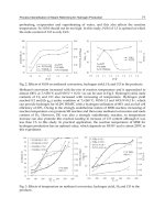
Fig. 2. Evaporation and transpiration and the factors that impact these processes in an
irrigated crop.
2. Evapotranspiration and energy budget
The estimation of ET parameter, corresponding to the latent heat flux (E) from remote
sensing is based on the energy balance evaluation through several surface properties such as
albedo, surface temperature (T
s
), vegetation cover, and leaf area index (LAI). Surface energy

balance (SEB) models are based on the surface energy budget equation. To estimate regional
crop ET, three basic types of remote sensing approaches have been successfully applied (Su,
2002).
The first approach computes a surface energy balance (SEB) using the radiometric surface
temperature for estimating the sensible heat flux (H), and obtaining ET as a residual of the

Evapotranspiration – Remote Sensing and Modeling
440
energy balance. The single-layer SEB models implicitly treat the energy exchanges between
soil, vegetation and the atmosphere and compute latent heat flux (E) by evaluating net (all-
wave) radiant energy (R
n
), soil heat flux (G) and H. For instantaneous conditions, the energy
balance equation is the following:
=

−− (1)
where: R
n
= net radiant energy (all-wave); G = soil heat flux; H = sensible heat flux (Wm
-2
);
E = latent energy exchanges (E = the rate of evaporation of water (kg m
-2
s
-1
) and  = the
latent heat of vaporization of water (J kg
-1
)). E is obtained as the residual of the energy

balance contain biases from both H and (R
n
- G). There are several factors which affect the
performance of single-source approaches, like the uncertainties about atmospheric and
emissivity effects. LST impacts on all terms of the energy balance in particular on long wave
radiation. The radiative surface temperatures provided by an infrared radiometer from a
space borne platform are measured by satellite sensors such as LANDSAT, AVHRR, MODIS
and ASTER. Converting radiometric temperatures to kinetic temperature requires
considerations about surface emissivity (E), preferably from ground measurements.
Remotely LST is subject to atmospheric effects which are primarily associated with the
absorption of infrared radiation by atmospheric water vapor and which lead to errors of 3–5
K. A wide range of techniques have been developed to correct for atmospheric effects,
including: single-channel methods; split-window techniques; multi-angle methods and
combinations of split-window and multi-channel methods. Radiant and convective fluxes
can be described: by considering the observed surface as a single component (single layer
approaches); by separating soil and vegetation components with different degrees of canopy
description in concordance with the number of vegetation layers (multilayer approaches).
Net radiant energy depends on the incident solar radiation (R
g
), incident atmospheric
radiation over the thermal spectral domain (R
a
), surface albedo (α
s
), surface emissivity (ε
s
)
and surface temperature (T
s
), according to the following equation:



=
(
1−

)


+



−




 (2)
For single layer models, R
n
is related to the whole surface and in the case of multiple layer
models, R
n
is linked with both soil and vegetation layers. For single approaches, sensible
heat flux H is estimated using the aerodynamic resistance between the surface and the
reference height in the lower atmosphere (usually 2 m) above the surface. Aerodynamic
resistance (r
a
) is a function of wind speed, atmospheric stability and roughness lengths for

momentum and heat. For multiple layer models, H is characterized taking into account the
soil and canopy resistance, with the corresponding temperature:
=

(



)


 (3)
Eq. (3) shows that the estimation of E parameter can be made using the residual method,
which induces that E is linearly related to the difference between the surface temperature
(T
s
) and air temperature (T
a
) at the time of T
s
measurement if the second order dependence
of r
a
on this gradient is ignored.
=

−−
(





)



 (4)
Possibilities of Deriving Crop Evapotranspiration from
Satellite Data with the Integration with Other Sources of Information
441
Equation (4) is usually used to estimate E. At midday, it provides a good indicator
regarding the plant water status for irrigation scheduling. For E estimation over longer
periods (daily, monthly, seasonal estimations), the use of ground-based ET from weather
data is necessary to make temporal interpolation. Some studies have used the trend for the
evaporative fraction (EF), such as the ratio of latent heat flux to available energy for
convective fluxes, to be almost constant during the daytime. This allows estimating the
daytime evaporation from one or two estimates only of EF at midday, for example at the
satellite acquisition time (Courault et al., 2005).
=




, 

=∗

 (5)
ET can be estimated from air vapor pressure (p
a

) and a water vapor exchange coefficient (h
s
)
according to the following equation:
=

ℎ

(


∗
(


)
−

)
 (6)
Usually this method is used in models simulating Soil–Vegetation–Atmosphere Transfers
(SVAT). p
s
∗
(T
s
) represent the saturated vapor pressure at the surface temperature T
s
and h
s

is the exchange coefficient which depends on the aerodynamic exchange coefficient (1/r
a
),
soil surface and stomatal resistances of the different leaves in the canopy. Katerji & Perrier
(1985) estimated a global canopy resistance (r
g
) including both soil and canopy resistances
(equation 6)


=
1
1


+

+
1


+


(7)
where: r
veg
is the resistance due to the vegetation structure, r
w

the resistance of the soil layer
depending on the soil water content, r
0
the resistance due to the canopy structure and r
s
the
bulk stomatal resistance. To calculate this parameters it necessary to have information
regarding the plant structure like LAI and fraction of vegetation cover (FC), the minimum
stomatal resistance (r
smin
). Many studies proposed various parameterizations of the stomatal
resistance taking into account climatic conditions and soil moisture (Jacquemin & Noilhan,
1990). This proves that the (T
s
− T
a
) is related to ET term, and that Ts can be estimated using
thermal infrared measurements (at regional or global scale using satellite data, and at local
scale using ground measurements).
The second approach uses vegetation indices (VI) derived from canopy reflectance data to
estimate basal crop coefficient (K
cb
) that can be used to convert reference ET to actual crop
ET, and requires local meteorological and soil data to maintain a water balance in the root
zone of the crop. The VIs is related to land cover, crop density, biomass and other
vegetation characteristics. VIs such as the Normalized Difference Vegetation Index (NDVI),
the Soil Adjusted Vegetation Index (SAVI), the Enhanced Vegetation Index (EVI) and the
Simple Ratio (SR), are measures of canopy greenness which may be related to physiological
processes such as transpiration and photosynthesis. Among the relatively new satellite
sensors it has to be mentioned the advantages of using MODIS/Aqua that offer improved

spectral and radiometric resolution for deriving surface temperatures and vegetation
indices, as well as increased frequency of evaporative fraction and evaporation estimates
when compared with other sensors. The observed spatial variability in radiometric surface

Evapotranspiration – Remote Sensing and Modeling
442
temperature is used with reflectance and/or vegetation index observations for evaporation
estimation. For ET estimation from agricultural crops the most direct application is to
substitute the VIs for crop coefficients (defined as the ratio between actual crop water use
and reference crop evaporation for the given set of local meteorological conditions).
Negative observing correlations between the NDVI and radiometric surface temperature
could be linked to evaporative cooling, although for most landscapes variations in fractional
vegetation cover, soil moisture availability and meteorological conditions will cause
considerable scatter in those relationships. The methods associated with this approach
generate spatially distributed values of K
cb
that capture field-specific crop development and
are used to adjust a reference ET (ET
o
) estimated daily from local weather station data.
The third approach uses remotely sensed LST with Land Surface Models (LSMs) and Soil–
Vegetation–Atmosphere (SVAT) models, developed to estimate heat and mass transfer at
the land surface. LSMs contain physical descriptions of the transfer in the soil–vegetation–
atmosphere continuum, and with proper initial and boundary conditions provide
continuous simulations when driven by weather and radiation data. The energy-based
LSMs are of particular interest because these approaches allow for a strong link to remote
sensing applications. The use of the spatially distributed nature of remote sensing data as a
calibration source has been limited, with the focus placed on data assimilation approaches to
update model states, rather than inform the actual model structure. Data assimilation is the
incorporation of observations into a numerical model(s) with the purpose of providing the

model with the best estimate of the current state of a system. There are two types of data
assimilation: (i) sequential assimilation which involves correcting state variables (e.g.
temperature, soil moisture) in the model whenever remote sensing data are available; and
(ii) variation assimilation when unknown model parameters are changed using data sets
obtained over different time windows. Remotely sensed LSTs have been assimilated at point
scales into various schemes for estimating land surface fluxes by comparing simulated and
observed temperatures and adjusting a state variable (e.g. soil moisture) or model
parameters in the land surface process model. Such use of remote sensing data has
highlighted problems of using spatial remote sensing data with spatial resolutions of tens or
hundreds of kilometers with point-scale SVAT models and has led to the search for
‘‘effective’’ land surface parameters. There exist no effective means of evaluating ET
spatially distributed outputs of either remote sensing based approaches or LSMs at scales
greater than a few kilometers, particularly over non-homogeneous surfaces. The inability to
evaluate remote sensing based estimates in a distributed manner is a serious limitation in
broader scale applications of such approaches. It must be noted here that ET evaluation of
remote sensing based approaches with ground based data tends to favour those few clear
sky days when fluxes are reproduced most agreeably, and on relatively flat locations.
In this case the radiation budget is given by the following equation (Kalma et al., 2008):


=↓−↑+↓−↑ (8)
where K is the down-welling shortwave radiation and it depends on atmospheric
transmissivity, time of the day, day of the year and geographic coordination. K represents
the reflected shortwave radiation which depends on K and surface albedo (a), L is the
down-welling long wave radiation and L is the up-welling long wave radiation. L
depends on the atmospheric emissivity (which in turn is influenced by amounts of
atmospheric water vapor, carbon dioxide and oxygen) and by air temperature. L si
influenced by land surface temperature and emissivity
Possibilities of Deriving Crop Evapotranspiration from
Satellite Data with the Integration with Other Sources of Information

443
3. Direct methods using difference between surface and air temperature
Mapping daily evapotranspiration over large areas considering the surface temperature
measurements has been made using a simplified relationship which assumes that it is
possible to directly relate the daily (E
d
) to the difference (T
rad
– T
a
)
i
between (near) mid-day
observations (i) of surface temperature and near-surface air temperature (Ta) measured at
midday as follows:


=
(


)

−
(


−

)



 (9)
B is a statistical regression coefficient which depends on surface roughness. n depends on
atmospheric stability. Equation 9 was derived from Heat Capacity Mapping Mission
(HCMM) observations over fairly homogeneous irrigated and non-irrigated land surfaces,
with areas between 50 and 200 km
2
(Seguin et al. 1982a, b). Some authors as Carlson et al.
(1995a) proposed a simplified method based on Eq. 9 which uses the difference (T
rad
– T
a
) at
50 m at the time of the satellite overpass. They showed that B coefficient and n are closely
related to fractional cover f
c
that can be obtained from the NDVI–T
rad
plots. B values vary
from 0.015 for bare soil to 0.065 for complete vegetation cover and n decreased from 1.0 for
bare soil to 0.65 for full cover.
4. Surface energy balance models
Surface energy balance models (SEBAL) assume that the rate of exchange of a quantity (heat
or mass) between two points is driven by a difference in potential (temperature or
concentration) and controlled by a set of resistances which depend on the local atmospheric
environment and the land surface and vegetation properties. In the review made by
Overgaard et al. (2006) regarding the evolution of land surface energy balance models are
described the following approaches: the combination approach by Penman (1948) which
developed an equation to predict the rate of ET from open water, wet soil and well-watered

grass based on easily measured meteorological variables such as radiation, air temperature,
humidity, and wind speed; the Penman–Monteith ‘‘one-layer’’, ‘‘one-source’’ or ‘‘big leaf’’
models (Monteith 1965) which recognize the role of surface controls but do not distinguish
between soil evaporation and transpiration; this approach estimates ET rate as a function of
canopy and boundary layer resistances; ‘‘two-layer’’ or ‘‘two-source’’ model such as
described by Shuttleworth and Wallace (1985) which includes a canopy layer in which heat
and mass fluxes from the soil and from the vegetation are allowed to interact; multi-layer
models which are essentially extensions of the two-layer approach.
4.1 The Penman–Monteith, ‘‘one-source’’ SEB models
The Penman–Monteith (PM) approach combines energy balance and mass transfer concepts
(Penman, 1948) with stomatal and surface resistance (Monteith, 1981). Most “one source”
SEB models compute E by evaluating R
n
, G and H and solve for E as the residual term in
the energy balance equation (see Eq. 10). The sensible heat flux (H) is given by:
=


(


−

)



(10)
Where:  = air density (kg*m
-3

); C
p
= specific heat of air at constant pressure (J kg
-1
K
-1
); T
ad
=
aerodynamic surface temperature at canopy source height (K); T
a
= near surface air

Evapotranspiration – Remote Sensing and Modeling
444
temperature (K); r
a
= aerodynamic resistance to sensible heat transfer between the canopy
source height and the bulk air at a reference height above the canopy (s m
-1
). The r
a
term is
usually calculated from local data on wind speed, surface roughness length and
atmospheric stability conditions. According to Norman and Becker (1995), the aerodynamic
surface temperature (T
ad
) represent the temperature that along with the air temperature and
a resistance calculated from the log-profile theory provides an estimate H. The key issue of
PM approach is to estimate an accurately sensible heat flux. T

ad
is obtained by extrapolating
the logarithmic air temperature profile to the roughness length for heat transport (z
oh
) or,
more precisely, to (d + z
oh
) where d = zero-plane displacement height. Usually, due to the
fact that T
ad
cannot be measured using remote sensing, it is replaced with T
rad
. As it is
demonstrated by Troufleau et al. (1997), for dense canopy T
rad
and T
ad
may differ with 1-2 K
and much more for sparse canopy. Surface temperature (T
rad)
is related to the kinetic
temperature by the surface emissivity () (Eq, 11) and it depends on view angle () (Norman
et. al, 2000). On the other hand T
ad
and aerodynamic resistance are fairly difficult to obtain
for non-homogenous land surfaces.


=




∗

(11)
The aerodynamic resistance r
a
can be calculated with the following equation:


=
1



−


−Ψ

−


−


−Ψ

−



(12)
where: k = 0.4 (von Karman’s constant); u = wind speed at reference height z (m s
-1
); d =
zero-plane displacement height (m); z
oh
and z
om
= roughness lengths (m) for sensible heat
and momentum flux, respectively; 
h
and 
m
= stability correction functions for sensible
heat and momentum flux, respectively; L = Monin-Obukhov length L (m). The 
h
= 0 and

m
= 0 if near surface atmospheric conditions are neutrally stable. Usually, the aerodynamic
resistance is estimated from local data, even that area averaging of roughness lengths is
highly non-linear (Boegh et al. 2002). Several studies, such as Cleugh at al. (2007) used these
equations for evapotranspiration landscape monitoring. Their approach estimates E at 16-
day intervals using 8-day composites of 1 km MODIS T
rad
observations and was tested with
3 years of flux tower measurements and was obtained significant discrepancies between
observed and simulated land surface fluxes, generated by the following factors: the
estimation of H with Eqs. 9 and 10 is not constrained by the requirement for energy

conservation; errors in z
oh
determination; use of unrepresentative emissivities; using time-
averages of instantaneous T
rad
, T
a
and R
n
, the non-linearity of Eq. 9 may cause significant
errors; standard MODIS data processing eliminates all cloud-contaminated pixels in the
composite period. Bastiaanssen et al. (1998a) developed a calibration procedure using image
data to account for the differences between T
aero
and T
rad
, which are important, mainly for
incomplete vegetation covers. Other authors, such as Stewart et al. (1994) and Kustas et al.
(2003a), made empirical adjustments to aerodynamic resistance, related to z
oh
(eq. 13).
=




(
Θ
)
−




−


(13)
where: T
rad
() =radiometric surface temperature (K) at view angle  derived from the
satellite brightness temperature; r
ex
= excess resistance (s m
-1
) (reflects differences between
Possibilities of Deriving Crop Evapotranspiration from
Satellite Data with the Integration with Other Sources of Information
445
momentum and sensible heat transfer. According to Stewart et al. (1994) r
ex
is function of the
ratio of roughness lengths for momentum z
om
and for sensible heat z
oh
and the friction
velocity u* (m s
-1
) (eq. 14):



=



∗
=






∗

(14)
where kB
-1
= dimensionless ratio determined by local calibration. Eq. 14 assumes that the
ratio z
om
/z
oh
may be treated as constant for uniform surfaces, although kB
-1
has been found
to be highly variable (Brutsaert 1999).
In the case of the one source Surface Energy Balance System (SEBS) (Su, 2002) the surface
heat fluxes are estimated from satellite data and available meteorological data. There are
three sets of input data in SEBS: the first set includes the following parameters: , , T

rad
,
LAI, fractional vegetation coverage and the vegetation height (if the vegetation information
is not explicitly available, SEBS can use as input data the Normalized Difference Vegetation
Index (NDVI)); the second set includes T
a
, u, actual vapour pressure (e
a
) at a reference
height as well as total air pressure; the third set of data consists of measured (or estimated)
K and L. For R
n
, G, and the partitioning of (R
n
- G) into H and E, SEBS use different
modules (Fig. 3): H is estimated using Monin–Obukhov similarity theory; in the case of u
and vegetation parameters (height and LAI) is used the Massman (1997) model to to
estimate the displacement height (d) and the roughness height for momentum (z
om
); the
equations proposed by Brutsaert (1982, 1999) are used when only the height of the
vegetation is available. The SEBS was successfully tested for agricultural areas, grassland
and forests, across various spatial scales. Several studies used flux tower method and data
from Landsat, ASTER ad Modis sensors (Su et al. 2005, 2007, McCabe and Wood 2006).
The Fig. 4 shows the time series, determined during the Soil Moisture Atmosphere Coupling
Experiment 2002 (SMACEX-02) (Kustas et al. 2005). These time series illustrates latent heat
fluxes and sensible heat fluxes measured with in situ eddy-covariance equipment (closed)
together with SEBS model (open) over a field site (corn) from Iowa. The gaps in the time
series are caused either the missing ancillary data or absence of flux measurements. Many
factors influence the single-source approach: there are uncertainties due to atmospheric and

emissivity effects; because of the vegetation properties and of the angle view, the
relationship between T
ad
and T
a
is not unique; this approach requires representative near-
surface T
a
and other meteorological data measured (or estimated) at the time of the satellite
overpass at a location closely with the T
rad
observation. This can generate errors in defining
meteorological parameter for each satellite pixel from a sparse network of weather stations
(at the time of satellite overpass), mainly for areas with high relative relief and slopes.
Another important factor is that the accuracy of any of the estimates depends on the
performance of the algorithm used for temperature retrieval.
The major advantages of SEBS are: uncertainty due to the surface temperature or
meteorological variables can be limited taking into account the energy balance at the
limiting cases; through the SEBS was formulated a new equation for the roughness height
for heat transfer, using fixed values; a priori knowledge of the actual turbulent heat fluxes is
not required. Another single-source energy balance models, developed based on the
conception of SEBAL, are S-SEBI (Simplified-SEBI), METRIC (Mapping EvapoTranspiration
at high Resolution with Internalized Calibration), etc. The main difference between such
kinds of models is the difference in how they calculate the sensible heat, i.e. the way to
define the dry (maximum sensible heat and minimum latent heat) and wet (maximum latent

Evapotranspiration – Remote Sensing and Modeling
446
heat and minimum sensible heat) limits and how to interpolate between the defined upper
and lower limits to calculate the sensible heat flux for a given set of boundary layer

parameters of remotely sensed data (T
s
, albedo, NDVI, LAI) and ground-based air
temperature, wind speed, humidity. The assumptions in all these models are that there are
few or no changes in atmospheric conditions (especially the surface available energy) in
space and sufficient surface horizontal variations are required to ensure dry and wet limits
existed in the study area.


Fig. 3. Schematic representation of SEBS (after Su, 2008)


Fig. 4. Reproduction of surface flux development with a one-source model (SEBS) (after
Kalma, 2008)
4.2 Two-source SEB models
The equations 10 and 13 make no difference between evaporation soil surface and
transpiration from the vegetation and from this reason the resistances are not well defined.
Possibilities of Deriving Crop Evapotranspiration from
Satellite Data with the Integration with Other Sources of Information
447
To solve this problem two-source models have been developed for use with incomplete
canopies (e.g. Lhomme et al. 1994; Norman et al. 1995; Jupp et al. 1998; Kustas and Norman
1999). These models consider the evaporation as the sum of evaporation from the soil
surface and transpiration from vegetation. For example, Norman et. Al. (1995) developed a
two-source model (TSM) based on single-time observations which eliminate the need for r
ex

as used in equations 13 and 14. They reformulated the equation 10 as:
=




(

)
−




(15)
where: T
rad
= directional radiometric surface temperature obtained at zenith view angle ; r
r
= radiometric-convective resistance (s m
-1
). The radiometric convective resistance is
calculated according to the following formula:


=


(

)
−



(


−

)


+
(


−

)


+



(16)
where: T
c
= canopy temperature; T
s
= soil surface temperature; R
s
= soil resistance to heat
transfer (s m-

1
). To estimate the T
c
and T
s
variables, Norman et al. used fractional vegetation
cover (fc) which depends on sensor view angle (Eq. 17):


(

)
≈



(

)



+

1−

(

)








 (17)
H variable is divided in vegetated canopy (H
c
) and soil (H
s
) influencing the temperature in
the canopy air-space. Other revisions of TSM compared flux estimates from two TSM
versions proved that thermal imagery was used to constrain T
rad
and H and microwave
remote sensing was employed to constrain near surface soil moisture. The estimations
resulting from those two models were compared with flux tower observations. The results
showed opposing biases for the two versions that it proves a combination between
microwave and thermal remote sensing constraints on H and E fluxes from soil and
canopy. Compared to other types of remote sensing ET formulations, dual-source energy
balance models have been shown to be robust for a wide range of landscape and hydro-
meteorological conditions.
5. Spatial variability methods using vegetation indices
Visible, near-infrared and thermal satellite data has been used to develop a range of
vegetation indices which have been related to land cover, crop density, biomass or other
vegetation characteristics (McVicar and Jupp 1998). Several vegetation indices as the
Normalized Difference Vegetation Index (NDVI), the Soil Adjusted Vegetation Index
(SAVI), the Enhanced Vegetation Index (EVI) and the Simple Ratio (SR), are indicators of
canopy greenness which can be related to physiological processes such as transpiration and

photosynthesis (Glenn et al., 2007).
5.1 Vegetation indices, reflectance and surface temperature
The SEBAL approach used remotely sensed surface temperature, surface reflectivity and
NDVI data. It has been developed for the regional scale and it requires few ground level
observations from within the scene. K and L are computed using a constant atmospheric

Evapotranspiration – Remote Sensing and Modeling
448
transmissivity, an appropriate atmospheric emissivity value and an empirical function of T
a
,
respectively. G is calculated as a fraction of R
n
depending on T
rad
, NDVI and  (Bastiaanssen
2000). The instantaneous values of sensible heat flux are calculated in three main steps. First
step makes the difference between T
ad
and T
rad
and assumes that the relationship between
T
rad
and the near-surface temperature gradient (T = T
ad
- T
a
) is quasi-linear. Therefore wet
and dry extremes can be identified from the image. These extremes fix the quasi-linear

relationship relating T to T
rad
, allowing T to be estimated for any T
rad
across the image. In
the second step, a scatter plot is obtained for all pixels in the entire image of broadband 
values versus T
rad
. Low temperature and low reflectance values correspond to pixels with
large evaporation rates, while high surface temperatures and high reflectance values
correspond to the areas with little or no evaporation rates. Scatter plots for large
heterogeneous regions frequently show an ascending branch controlled by moisture
availability and evaporation rate, and a radiation-controlled descending branch where
evaporation rate is negligible. The ascending branch indicates that the temperatures increase
with increasing  values as water availability is reduced and evaporation rate becomes more
limited. For the descending branch the increasing of  induce a decreasing of surface
temperature. If the radiation-controlled descending branch is well defined, r
a
may be
obtained from the (negative) slope of the reflectance–surface temperature relationship. The
last step use the local surface roughness (z
om
) based on the NDVI; is assumed that the
z
om
/z
oh
ratio has a fix value and H can be calculated for every pixel with E as the residual
term in Eq. 1. The SEBAL models have been used widely with satellite data in the case of
relatively flat landscapes with and without irrigation.

The Mapping EvapoTranspiration with high Resolution and Internalized Calibration
(METRIC) models, derived from SEBAL are used for irrigated crops (Allen et al. 2007a, b).
METRIC model derive ET from remotely sensed data (LANDSAT TM) in the visible, near-
infrared and thermal infrared spectral regions along with ground-based wind speed and
near surface dew point temperature. In this case extreme pixels are identified with the
cool/wet extreme comparable to a reference crop, the evaporation rates being computed
wit Penman-Monteith method. The ET from warm/dry pixel is calculated using soil water
budget having local meteorological data as input parameters. METRIC model can be used
to produce high quality and accurate maps of ET for areas smaller than a few hundred
kilometers in scale and at high resolution (Fig. 5). In their study, Boegh et al. (1999)
presented an energy balance method for estimating transpiration rates from sparse
canopies based on net radiation absorbed by the vegetation and the sensible heat flux
between the leaves and the air within the canopy. The net radiation absorbed by the
vegetation is estimated using remote sensing and regular meteorological data by merging
conventional method for estimation of the land surface net radiation with a ground-
calibrated function of NDVI.
SEBAL and METRIC methods assume that the temperature difference between the land
surface and the air (near-surface temperature difference) varies linearly with land surface
temperature. Bastiaanssen et al. (1998) and Allen and al. (2007) derive this relationship
based on two anchor pixels known as the hot and cold pixels, representing dry and bare
agricultural fields and wet and well-vegetated fields, respectively. Both methods use the
linear relationship between the near-surface temperature difference and the land surface
temperature to estimate the sensible heat flux which varies as a function of the near-surface
temperature difference, by assuming that the hot pixel experiences no latent heat, i.e., ET =
0.0, whereas the cold pixel achieves maximum ET.
Possibilities of Deriving Crop Evapotranspiration from
Satellite Data with the Integration with Other Sources of Information
449

Fig. 5. (a) Landsat color infrared image of T3NR1E of the Boise Valley; (b) Land use/land

cover polygons in T3NR1E of the Boise Valley; (c) ET image of T3NR1E the Boise Valley
(after R.G. Allen et al., 2007)
The sensible heat flux is assessed like a linear function of the temperature difference
between vegetation and mean canopy air stream. The surface temperature recorded by
satellite comprises information from soil and from vegetation; therefore the vegetation
temperature is estimated taking into account the linear relationship between NDVI and
surface temperature. The difference between the surface temperature and the mean canopy
air stream temperature is linearly related to the difference between surface temperature
and the air temperature above the canopy with the slope coefficient which depend on the
canopy structure. This relationship was used to evaluate the mean canopy air stream
temperature. The method was used in the Sahel region for agricultural crops, natural
vegetation, forest vegetation, with ground based, airborne and satellite remote sensing
data and validated with sapflow and latent heat flux measurements. Agreement between
remote sensing based estimates and ground based measurements of E rates is estimated
to be better than 30–40 W m
-2
.
5.2 Reflectance and surface temperature
The Simplified Surface Energy Balance Index (S-SEBI) proposed by Roerink et al. (2000)
estimate the instantaneous latent heat flux (E
i
) with (Kalma, 2008):


=Λ

(


−


)
 (18)
where: (R
ni
– G
i
) = available energy at the time of the satellite overpass; 
i
= the evaporative
fraction. The S-SEBI algorithm has two limitations: the atmospheric conditions have to be
almost constant across the image and the image has to contain borh dry and wet areas. 
i

was obtained from a scatter plot of observed surface temperature (T
rad
) and Landsat TM
derived broadband a values across the single scene. 
i
is with:
Λ

=


−



−



(19)
where: T
rad
= observed surface temperature for a given pixel; T
H
= temperature for the
upper boundary (dry radiation controlled conditions - all radiation is used for surface
heating and  decreases with increasing surface temperature (T
H
- where E = 0 (W m
-2
));
T

E
= temperature at the lower boundary (evaporation controlled wet conditions - all energy

Evapotranspiration – Remote Sensing and Modeling
450
is used for E and  increases with an increase of surface temperature (T

E
-where H = 0 W
m
-2
)). This method does not need any additional meteorological data.

Fig. 6. Flowchart of the proposed methodology to obtain ET from NOAA–AVHRR data
(after Sobrino et al., 2007)
Sobrino et. al (2007) use S-SEBI algorithm to estimate the daily evapotranspiration from
NOAA-AVHRR images for the Iberian Penisnula. The Figure 6 present the flowchart used
by Sobrino et al. (2007) to obtain ET from NOAA-AVHRR. Daily evapotranspiration (ET
d
) is
given by:


=
Λ







(20)
where: R
nd
= daily net radiation; R
ni
= instantaneous net radiation: L = 2.45 MJ kg
-1
= latent
heat vaporization; C
di
=R

nd
/R
ni
. In this case the daily ground heat flux was considered close
to 0. There are several studies which proposed methods for C
di
calculation. For example
Seguin and Itier (1983) proposed a constant value for C
di
= (0.30±0.03). Wassenaar et al.
(2002) showed that this ratio have a seasonal variation 0.05 in winter to 0.3 in summer,
following a sine law. In the Sobrino et al. (2007) study, C
di
was calculated using net radiation
fluxes measured at the meteorological station of located on the East coast of the Iberian
Peninsula (El Saler area). The ET estimation from high spectral and spatial resolution data
(5 m) was adapted to the low resolution data NOAA-AVHRR (1 km spatial resolution)
based on the evaporative fraction concept proposed by Roerink et al. (2007). The main
Possibilities of Deriving Crop Evapotranspiration from
Satellite Data with the Integration with Other Sources of Information
451
advantage of the Sobrino et al. (2007) methodology is that the method requires only satellite
data to estimate ET.


Fig. 7. Monthly evolution (from June 1997 to November 2002) of the daily
evapotranspiration (ET
d
) in the eight selected zones. There is represented also the temporal
mean for the six years of analyzing (after Sobrino et al., 2007).

Its major disadvantage is represented by the requiring that satellite images must have
extreme surface temperatures. The method was tested over agricultural area using high
resolution values, with errors lower than 1.4 mm d
-1
. As it can be observed from Fig. 7,
regarding the monthly and seasonal evolution of ET the highest values (∼6 mm d
−1
) were
obtained in the West of the Iberian Peninsula, which is the most vegetated area. Taking into
account the impact of incoming solar energy the higher values of ET was obtained in spring
and summer and the lower values in autumn and winter. Seasonal ET was obtained by
averaging daily ET over the season. Figure 8 shows as an example the monthly ET maps
obtained from the NOAA-AVHRR images acquired in 1999. Fig. 9 also indicates that the
highest ET values were obtained in the summer and spring, in the north and west of Iberian
Peninsula. To map land surface fluxes and surface cover and surface soil moisture, Gillies
and Carlson (1995) combined two model, SVAT and ABL and run it for vegetative cover
with the maximum known NDVI and for bare soil conditions with the minimum known
NDVI in the scene for a range of soil moisture values until AVHRR observed (T
rad
) and
simulated (T
ad
) surface temperatures corrected, at which stage the actual fractional
vegetation cover (f
c
) and surface soil moisture were estimated.

Evapotranspiration – Remote Sensing and Modeling
452

Fig. 8. Monthly mean for the daily evapotranspiration obtained from NOAA–AVHRR data
over the Iberian Peninsula in 1999. Pixels in black color correspond to sea and cloud masks
and red correspond to higher value of ET (after Sobrino et al., 2007).
5.3 Vegetation indices and surface temperature
Several studies shown the efficiency of ‘‘triangle method’’ (Carlson et al. (1995a, b); Gillies et
al. 1997; Carlson 2007) to estimate soil moisture from the NDVI–T
rad
relationship. The major
advantages of the remotely sensed VI-T
s
triangle method are that: the method allows an
accurate estimation of regional ET with no auxiliary atmospheric or ground data besides the
remotely sensed surface temperature and vegetation indices; is relatively insensitive to the
correction of atmospheric effects. Its limitations are: determination of the dry and wet edges
requires a certain degree of subjectivity; to make certain that the dry and wet limits exist in
the VI-T
rad
triangle space most of pixels over a flat area with a wide range of soil wetness
and fractional vegetation cover are required. So, the boundaries of this triangle are limiting
conditions for H and E. Other studies suggest the dependence of T
rad
variability on the
remote sending data resolution, thus higher resolution data means that the variations of T
rad

and NDVI is more related to the land cover type. Lower resolution data show the
dependency of the NDVI and T
rad
variations to agricultural practices and rainfall. Jiang and
Islam (2001) proposed a triangle method based on the interpolation of the Priestley–Taylor

method (Priestley and Taylor, 1972) using the triangular (T
rad
, NDVI) spatial variation. The
Priestley–Taylor expression for equilibrium evaporation from a wet surface under
conditions of minimal advection (E
PT
) is given by:


=

(


−
)


(21)
Possibilities of Deriving Crop Evapotranspiration from
Satellite Data with the Integration with Other Sources of Information
453
where:  = slope of the saturated vapour pressure curve at the prevailing Ta ((Pa K
-1
);  =
psychrometric constant (Pa K
-1
); 
PT
= Priestley-Taylor parameter defined as the ratio

between actual E and equilibrium E. For wet land surface conditions, 
PT
= 1.26. Its value is
affected by global changes in air temperature, humidity, radiation and wind speed. Jiang
and Islam (2001) replaced 
PT
with parameter  which varies for a wide range of r
a
and r
c

values. The warm edge of the (T
rad
, NDVI) scatter plot represents pixels with the highest T
rad

and minimum evaporation from the bare soil component, while E
a
can vary function of the
vegetation type. Linear interpolation between the sides of the triangular distribution of T
rad
-
NDVI allows to derive  for each pixel using the spatial context of remotely sensed T
rad
and
NDVI. The  values are related to surface wetness, r
s
and T
rad
. Therefore, the minimum

value of  is 0 for the driest bare soil pixel and the maximum value is 1.26 for a densely
vegetated, well-watered pixel. Thus the actual  value for each pixel in a specified NDVI
interval is obtained from the observed (T
rad
)
obs
with the following:
=

(


)

−
(


)

(


)

−
(


)



(22)
where (T
rad
)
min
and (T
rad
)
max
are the lowest and highest surface temperatures for each NDVI
class, corresponding to the highest and lowest evaporation rates, respectively. The
evaporative fraction can be calculated with:
Λ=



(23)
Based on the Jiang and Islam (2001) approach, Wang et al. (2006) obtained better results
using the spatial variation (T
rad
, NDVI), where T
rad
represent the day–night difference in
T
rad
, obtained from MODIS data. However, to convert  into E, the method described above
still requires estimation/ measurement of net radiation (R
n

) and soil heat flux (G). In a later
work, Jiang and Islam (2003) consider the fractional vegetative cover (f
c
) as a more suitable
generalized vegetation index calculated from the normalized NDVI with (Kalma et al. 2008):


=
− 



− 




(24)
They assumed that the evaporative fraction  = E/(R
n
- G) is linearly related to T = T
rad
-
T
a
, inside a certain class f
c
. The reason for this assumption is that theT is more
representative for sensible heat flux H. Thus the evaporative fraction can be estimated from
f

c
and T, for a given set of T
max
, T
e
(T
e
= T
max
for f
c
= 1) and a stress factor (). In their
study, they used NOAA-AVHRR data and obtained better results using the aerodynamic
resistance-energy balance method represented by Eq. 13, this equation including
atmospheric stability corrections and using an iterative procedure to reach the most
appropriate kB
-1
value.
Serban et al. (2010) used the Priestly-Taylor equation modified by Jiang and Islam (2001) in
their study to estimate the evapotranspiration using remote sensing data and Grid
Computing. The most advantage of Priestly-Taylor equation is that the all terms can be
calculated using remotely sensed data. Grid computation procedure has two major
advantages: strong data processing capacity and the capability to use distributed computing
resources to process the spatial data offered by a satellite image. According to Jiang and
Islam (2001) the parameter α
PT
parameter is obtained by two-step linear interpolation: in the

Evapotranspiration – Remote Sensing and Modeling
454

first step is obtained upper and lower bounds of α
PT
for each specific NDVI class
(determined from the land use/land cover map); in the second step the parameter α
PT
is
ranged within each NDVI class between the lowest temperature pixel and the highest
temperature pixel. According to land use/land cover map, for this paper, was considered
four main land uses: vegetation, water, barren land and urban. Each NDVI value
corresponds to a certain NDVI class. In this case the relationship between LST and NDVI is
used. Thus, the parameter α
PT
is calculated with:


=
∆+
∆




−



−







−





+
∆+
∆









(25)
where: LST = surface temperature for current pixel; LST
i
max
and LST
i
min
= maximum and
minimum surface temperature within NDVI class which has the current pixel; NDVI

i
max
and
NDVI
i
min
are the maximum and minimum NDVI within NDVI class which has the current
pixel. They calculated the daily value of ET with the following (Fig. 9):


=

2
(


−

)





(26)
where: DL = total day length (hours); t = time beginning at sunrise. To obtain the 24 hours
totals, the daily ET values are multiplied by 1.1 for all days. LST was computed using
Jimenez- Munoz and Sobrino’s algorithm which requires a single ground data (the total
atmospheric water vapor content – w) (Fig. 10):
=




(




+

)
+


+ (27)
=















+


(28)
=

+

 (29)


=∗+− (30)


=







+1

(31)
where: LSE = land surface emissivity = 1.0094+0.047*ln(NDVI);  = effective wavelength;
DN = digital number of a pixel; T
sesnor
= brightness temperature; c
1

= 1.19104*10
8
Wμm
4
m
-
2
sr
-1
; c
2
= 14387.7μmK; 
i
(i = 1, 2, 3) = atmospheric parameters, which depend on total
atmospheric water vapor content (w). Besides satellite data, this study uses two ground
meteorological data: the total atmospheric water vapor content - w, used in LST estimation
algorithm, and the air temperature - T
air
. To estimate evapotranspiration, Serban et al. (2010)
used one subset of Landsat ETM+ (7th June 2000) for Dobrogea area corresponding to
Constanta weather station, which was atmospherically corrected.
From the bands ETM+ 3 and 4 were analyzed the NDVI values, the band ETM+ 6 was
processed to determine LST, and the other bands (ETM+ 1, 2, 5 and 7) were used to estimate
the albedo values. The difference between the actual mean soil surface temperature at the
Possibilities of Deriving Crop Evapotranspiration from
Satellite Data with the Integration with Other Sources of Information
455
time when satellite passed and the remote sensed mean land surface temperature (0.73
O
C) is

considered acceptable. The evapotranspiration (Fig. 10) ranges between 0.33 and
5.24mm/day. According to Constanta weather station, the multi-annual average of the
evapotranspiration in June is between 4.5 and 5.6 mm/day, so the estimation error is
eligible.


Fig. 9. LST Image - Dobrogea region, 2000 (After Serban et al., 2010)


Fig. 10. ETP Image - Dobrogea region, 2000 (After Serban et al., 2010)
6. ET estimation using meteorological data
6.1 Crop evapotranspiration
At a crop level, ET may not occur uniformly because variations in crop germination, soil water
availability, and other factors such as non-uniform water and nutrient applications and an
uneven distribution of solar radiation within the canopy. Usually, the top leaves are more
active in transpiration than the lower leaves because they receive more light. Also, the bottom
leaves mature and age earlier and they may have lower transpiration rates than the greener
and younger top leaves. Thus, weather parameters, crop characteristics, environmental and
management aspects are the factors which influence the evaporation and transpiration

Evapotranspiration – Remote Sensing and Modeling
456
processes. The main weather parameters influencing evapotranspiration are radiation, air
temperature, humidity and wind speed. Several algorithms have been developed to estimate
the evaporation rate from these parameters. The evaporation power of the atmosphere is
expressed by the reference crop evapotranspiration (ET
o
) which represents the
evapotranspiration from a standardized vegetated surface (Allen et al., 1998). The reference
surface is a hypothetical grass reference crop with specific characteristics. Because ET

o
is
affected by only climatic parameters, it is a climatic parameter and may be computed from
weather data. Thus ET
o
is the evaporating power of the atmosphere at a specific location and
time of the year and does not take into account the crop characteristics and soil factors.
Crop water requirement is defined as the amount of water required to compensate the
evapotranspiration loss from the cropped field. Even the values for crop evapotranspiration
are identical with crop water requirement (CWR), crop evapotranspiration refers to the
amount of water that is lost by evapotranspiration, while CWR refers to the amount of water
that needs to be supplied. Thus, the irrigation water requirement represents the difference
between the crop water requirement and effective precipitation and also includes additional
water for leaching of salts and to compensate for non-uniformity of water application (Allen et
al., 1998). Several empirical methods have been developed over the last five decades in order
to estimate the evapotranspiration from different climatic variables. Testing the accuracy of the
methods under a new set of conditions is laborious, time-consuming and costly, and yet
evapotranspiration data are frequently needed at short notice for project planning or irrigation
scheduling design. To meet this need, guidelines were developed and published in the FAO
Irrigation and Drainage Paper No. 24 'Crop water requirements'. From different data
availability, four methods are usually used to estimate the reference crop evapotranspiration
(ET
o
): the Blaney-Criddle, radiation, modified Penman and pan evaporation methods. From
these four methods, the modified Penman-Monteith method offer the best results with
minimum possible error in relation to a living grass reference crop. The radiation method can
be used for areas where available climatic data include measured air temperature and
sunshine, cloudiness or radiation, but not measured wind speed and air humidity. The Blaney-
Criddle method is better to be applying for areas where available climatic data cover air
temperature data only. The pan method gives acceptable estimates, depending on the location

of the pan. Based on the original Penman- FAO proposed a standard parameterization of the
Penman–Monteith method for estimating the evaporation from a -irrigated, homogenous, 0.12
m grass cover considered as a ‘‘reference crop’’ (Allen et al., 1998) (Fig. 11).


Fig. 11. Characteristics of the hypothetical reference crop (after Allen et al., 1998)
Possibilities of Deriving Crop Evapotranspiration from
Satellite Data with the Integration with Other Sources of Information
457
Monteith equation and the equations of the aerodynamic and surface resistance, the FAO
Penman-Monteith method to estimate ET
o
is the following:


=
0.408∆
(


−
)
+
900
+273


(



−

)
∆+
(
1+0.34

)

(32)
where: ET
0
= reference evapotranspiration [mm day
-1
]; R
n
= net radiation at the crop surface
[MJ m
-2
day
-1
]; G = soil heat flux density [MJ m
-2
day
-1
]; T = mean daily air temperature at 2
m height [°C]; u
2
= wind speed at 2 m height [m s
-1

]; e
s
= saturation vapour pressure [kPa];
e
a
= actual vapour pressure [kPa]l; e
s
- e
a
= saturation vapour pressure deficit [kPa];  =
slope vapour pressure curve [kPa °C
-1
]; γ = psychrometric constant [kPa °C
-1
]. The equation
uses standard climatological records of solar radiation (sunshine), air temperature, humidity
and wind speed. To obtain correct estimations of ET
0
, the weather measurements should be
made at 2 m (or converted to that height) above an extensive surface of green grass, shading
the ground and not short of water. The psychrometric constant, γ, is calculated with:
=




=0.665∗10

(33)
Where: P = atmospheric pressure [kPa]; λ = latent heat of vaporization, 2.45 [MJ kg

-1
]; c
p
=
specific heat at constant pressure, 1.013 10-3 [MJ kg
-1
°C
-1
]; ε = ratio molecular weight of
water vapour/dry air = 0.622. For standardization, T
mean
for 24 hour is defined as the mean
of the daily maximum (T
max
) and minimum temperatures (T
min
) rather than as the average of
hourly temperature measurements.


=





 (34)
The temperature is given in degrees Celsius (°C), Fahrenheit (°F) or in Kelvin (K =C + 273,16).
=101.3
.




 (35)
where: z = elevation above sea level [m].
6.2 CROPWAT model
CROPWAT is a decision support system developed by the Land and Water Development
Division of FAO for planning and management of irrigation. The main functions of
CROPWAT model are: to calculate the reference evapotranspiration, crop water
requirements and crop irrigation requirements; to develop irrigation schedules under
different management conditions and water supply schemes; to estimate the rainfed
production and drought effects; to evaluate the efficiency of irrigation practices.
The input data of the model are the following climatic, crop and soil data: reference crop
evapotranspiration: (ET
o
) values measured or calculated using the FAO Penman–Montieth
equation based on monthly climatic average data of the minimum and maximum air
temperature (C), relative humidity (%), sunshine duration (h) and wind speed (m/s);
rainfall data: (daily/monthly data); monthly rainfall is divided for each month into a
number of rainstorms; a cropping pattern: crop type, planting date, crop coefficient data
files (including K
c
values, stage days, root depth, depletion fraction, K
y
values) and the area
planted (0– 100% of the total area); a set of typical crop coefficient data files are provided in
the program; soil type: total available soil moisture, maximum rain infiltration rate,

Evapotranspiration – Remote Sensing and Modeling
458

maximum rooting depth, and initial soil moisture depletion (% of the total available
moisture);scheduling criteria: several options can be selected regarding the calculation of the
application timing and application depth.
The output parameters for each crop are crop reference crop evapotranspiration Et
0

(mm/period), crop K
c
(average values of crop coefficient for each time step, effective rain
(mm/period) (the amount of water that enters in the soil); water requirements (CWR) or
ET
m
(mm/period); irrigation requirements (IWR - mm/period); actual crop
evapotranspiration (ET
c
- mm); effective rain (mm/period) which represents the amount of
water that enters into the soil; daily soil moisture deficit (mm); estimated yields reduction
due to crop stress (when ET
c
/ET
m
falls below 100%).
The CROPWAT model can compute the actual evapotranspiration using the FAO Penman–
Monteith equation or using directly the evapotranspiration measurements values. The crop
water requirements (CWR) or maximum evapotranspiration (ET
m
) (mm/period) are
calculated as:
=


∗

 (36)
This means that the peak CWR in mm/day can be less than the peak Et
o
value when less
than 100% of the area is planted in the cropping pattern.
The average values of the crop coefficient (K
c
) for each time step are estimated by linear
interpolation between the K
c
values for each crop development stage. The ‘‘Crop K
c
” values
are calculated as:


=

∗ (37)
where CropArea is the area covered by the crop. So, if the crop covers only 50% of the area,
the “Crop Kc” values will be half of the Kc values in the crop coefficient data file.
The CROPWAT model operates in two modes: computing the actual evapotranspiration
using climatic parameters and using directly the evapotranspiration measurements values.
Possibilities to use the satellite-based data as input into the CROPWAT model are limited,
because this model was not developed to use satellite-derived information directly. But this
information can be useful for the comparison/validation procedures of some model
input/output data, as precipitation, sunshine duration and evapotranspiration. Satellite
based data can be used by CROPWAT model in different ways: measured

evapotranspiration may be replaced with estimations derived from satellite data; for
comparison and validation procedures; satellite-derived evapotranspiration values may
bring better accuracy for the specialization of the punctual computing values; satellite
information may be used for the assessment of the some reference parameters of the actual
evapotranspiration (e.g. Land surface temperature, vegetation indexes, etc.).
6.3 Using earth observation data and CROPWAT model to estimate the actual crop
evapotranspiration
There is a strong dependence between evapotranspiration and surface temperature on the,
thus thermal images meteorological satellites (METEOSAT, NOAA, MODIS, LANDSAT)
adequate for mapping of regional evapotranspiration. Several works have been done to
determine regional evapotranspiration from satellite data (Batra et al., 2006; Courault et al.,
2005; Wood et al., 2003). The application of NOAA AVHRR data seems to be more
successful because of the higher spatial and spectral resolution (Stancalie et al., 2010).
Multichannel algorithms are routinely used for atmospheric correction of the AVHRR data.
Possibilities of Deriving Crop Evapotranspiration from
Satellite Data with the Integration with Other Sources of Information
459
Efforts are directed towards the estimation of surface temperatures by considering the
effects of emissivity (Lagouarde and Brunet, 1991; Li and Becker, 1993). The method used for
the estimation of the daily crop actual evapotranspiration, ET
cj
, is based on the energy
balance of the surface. The method uses the connection between evapotranspiration, net
radiation and the difference between surface and air temperatures measured around 14:00 h
(the time of the satellite passage), local time. The first version of the method used a
simplified linear relationship as:


−


=−∗
(


−

)
 (38)
where R
nj
is the daily net radiation; T
s
and T
amax
is the surface and air maximum
temperature; A, B are coefficients which depend on the surface type and the daily mean
wind speed. Coefficients A and B may be determined either analytically, on the basis of the
relationships given by Lagouarde and Brunet (1991), or statistically. The coefficients A and B
are stable in the case of mature crop vegetation cover and in clear sky conditions. The
coefficient B vary considerably, function of the land vegetation cover percent. In case of soil
with great thermal inertia, the heat flux changed by conduction at the soil-atmosphere
interface can be neglected and the computing relationship for daily actual crop
evapotranspiration can be expressed in a version 2 of the proposed method:


=

−

∗

(


−

)
 (39)


=0.0253+
.

(
/
)
 (40)
ℎ=

1−
(
−
)

−


 (41)
where: v = daily average wind speed; zh = vegetation roughness and LAI the foliar index.
One possible use of satellite information is to replace the measured evapotranspiration by
estimations made from satellite information. Because the estimations made from satellite

information are available only for clear sky conditions, it was not possible to estimate the
monthly average evapotranspiration, as input data in the CROPWAT model. For this
reason, the satellite-derived data have been used for comparison/validation procedures of
the CROPWAT model output data, like evapotranspiration. Fig. 12 presents the comparison
between daily crop evapotranspiration values computed by the CROPWAT model and
those computed through the energy balance method (Version 1), using remotely sensed data
at the Alexandria and Craiova test-areas (situated in the south-western part of Romania), in
the conditions of the year 2000 (Stancalie et al., 2010, 2010).
Analysis of model results concerning comparison of daily actual crop evapotranspiration
calculated by using climatic data vs. satellite estimations based on the surface energetic
balance (Version 1) showed that ET
c
values from satellite information are in general higher
than those simulated by the model, the differences being from +0.45 - 1.9 mm/day.
Preliminary results highlighted a good correlation between the simulated values
(CROPWAT) and those derived from the satellite data; with relative errors from +20% - 18%
at Craiova site and from +13% -17% at Alexandria site (Stancalie et al., 2010).
Fig. 13 shows a comparison between ET
c
simulated daily by the CROPWAT model over the
whole maize-growing season and by the energy balance method (Version 2) respectively,
using satellite data, at Alexandria and Craiova test-areas. The ET
c
calculated by the model is
very similar to the estimated one. The results obtained can constitute the premise of an ET
c

data validation process, determined by the CROPWAT model (Stancalie et al., 2010).

Evapotranspiration – Remote Sensing and Modeling

460

Fig. 12. Comparison between daily crop evapotranspiration values computed by the
CROPWAT model and by the energy balance method (Version 1) using satellite data at the
Alexandria and Craiova test-areas (after Stancalie et al., 2010)

Fig. 13. Comparison between daily crop et values computed by the CROPWAT model and
by the energy balance method (Version 2) using satellite data, at Alexandria (A) and Craiova
(B) test-areas, for the maize vegetative development period in 2000 (Stancalie et al., 2010).
Possibilities of Deriving Crop Evapotranspiration from
Satellite Data with the Integration with Other Sources of Information
461
7. Conclusions
The use of the multispectral satellite data can improve the classical methods applied in
determining the agrometeorological parameters, including evapotranspiration.
Estimating evapotranspiration using remote sensing methodologies have a significant role
in irrigation management and crop water demand assessment, for plant growth, carbon and
nutrient cycling and for production modeling in dry land agriculture and forestry. Also it
can have an important role in catchment hydrology, and larger scale meteorology and
climatology applications. In the last years, due to the exceptional developments of satellite
technology, a wide range of remote sensing-based evapotranspiration (ET) methods/models
have been developed and evaluated. The use of remote sensing data for ET estimation is
mainly based on land surface temperature (LST) and reflectivity (using different spectral
regions) due to satellite ability to spatially integrate over heterogeneous surfaces at a range
of resolutions and to routinely generating areal products once long time-series data
availability issues are overcome. The chapter reviews some main methods for estimating
crop evapotranspiration based on remotely sensed data, and highlights uncertainties and
limitations associated with those estimation methods. This paper is focused on Surface
Energy Balance models (SEB), spatial variability methods using vegetation indices and ET
estimation using meteorological data through CROPWAT model. The analysis and critical

issues are supported by the dedicated literature and specific case-studies. This review
provides information of temporal and spatial scaling issues associated with the use of
optical and thermal remote sensing for estimating evapotranspiration. Improved temporal
scaling procedures are required to extrapolate estimates to daily and longer time periods
and gap-filling procedures are needed when temporal scaling is affected by intermittent
satellite coverage. It is also noted that analysis of multi-resolution data from different
satellite/sensor systems is able to assist the development of spatial scaling and aggregation
approaches. Approaches differ in: (i) type and spatial extent of application (e.g. irrigation,
dry-land agriculture); (ii) type of remote sensing data; and (iii) use of ancillary (micro-)
meteorological and land cover data. The integration of remotely sensed data into
methods/models of ET facilitates the estimation of water consumption across agricultural
regions. There are important limitations for using remote sensing data in estimating
evapotranspiration.
Usually evapotranspiration is computed using land surface temperature and air
temperatures. All this methods are affected by errors induced by estimation or
measurements of those temperatures. The accuracy of T
rad
observations is influenced by
atmospheric factors, surface emissivity or view angle. Emissivity information is useful in
estimating of the radiative temperature of the land surface. Several direct methods (which
atmospheric variables are coupled with radiative transfer models) or indirect algorithms
(use only remote sensing data) to make atmospheric corrections in order to obtain the
brightness temperature that represents the temperature of a black body that would have the
same radiance as that observed by the radiometer. The uncertainties of surface temperature
have a strong influence in determination of sensible heat flux H. The difference between
surface and air temperatures depends on many factors, including vegetation type, fractional
cover f
c
and view angle. Another important limitation of various spatial variability methods
is considered the fact according to the highest and lowest surface temperatures observed in

the one scene are assumed to represent very dry and very wet pixels. Usually the available
energy (R
n
- G) is obtained from ground based point observations of R
n
: R
n
is estimated

Evapotranspiration – Remote Sensing and Modeling
462
based on observations of K, , LAI, emissivity of land surface and atmosphere, and T
rad
.
Such kind of estimation generates errors in the calculation of long and short wave
components. G can be estimated for example as function of NDVI. An alternative method
would be to assume that soil heat flux is a constant fraction of net radiation flux, but this
estimation doesn’t take into account the diurnal variation. Many models for ET estimation
need ground based meteorological data, mainly air temperature and wind speed. For that
models which based on computing the difference between Tad and Ta, the time and location
of air temperature (Ta) observations and their spatial representativeness are very
important).
Incomplete vegetation cover generates also errors in evapotranspiration estimation. The two
source models require parameterizations for the segmentation of the computed surface
temperature between vegetation and soil, for the turbulent exchange of heat and mass
between soil and atmosphere and between vegetation and atmosphere. Also, these models
require some assumptions regarding solar transmittance, extinction coefficients and canopy
emissivity in order to compute the variation of net radiation flux inside the canopy.
Another important limitation, regarding the spatial variability methods is that a large
number of pixels are required over the area of interest with a wide range of soil wetness and

fractional vegetation cover. The identification of vegetation limits for bare soil or full
vegetation cover can be easily done using high resolution images which display a wide
range in surface wetness conditions and land cover conditions
Remote sensing data is a useful tool that provides input data in land surface model (NDVI,
LAI, f
c
– fraction cover) and can be used to correct the state variables of the models.
The frequency of spatial resolution imagery is also very significant: satellites which
provide high resolution data usually have lower temporal frequency while low spatial
resolution images have higher temporal frequency. Some applications require different
spatial and temporal coverage rates and need different ‘‘turn-around’’ times. If acquiring
the satellite data and ET estimation method are more time consuming, the method are not
very convenient for operational applications like determining water requirements for
irrigated agriculture.
Another significant limitation for using remote sensing is the presence of clouds that
generates intermittent coverage. Cloudy days are characterized by a diffuse light, whereas
while direct light is dominant on clear days when most TIR data are acquired for use in
modeling applications. Most SEB models have been developed for use in cloud-free
conditions and do not makes difference between direct and diffuse radiation; they use only
daytime data obtained for clear-sky conditions. For a continuously monitoring of water
balance, the effects of an increased diffuse fraction should be taking into account, because
the diffuse radiation is used by vegetation more efficiently than direct radiation. For water
use efficiency, to ignore difference between direct and diffuse radiation can induce
significant differences in ET estimations.
8. References
Allen RG, Pereira LS, Raes D, Smith M (1998), Crop evapotranspiration - guidelines for
computing crop water requirements. FAO irrigation and drainage paper 56, Rome,
Italy
Possibilities of Deriving Crop Evapotranspiration from
Satellite Data with the Integration with Other Sources of Information

463
Allen RG, Tasumi M, Trezza R (2007a) Satellite-based energy balance for mapping
evapotranspiration with internalized calibration (METRIC): model. J Irrig Drain
Eng 133(4):380–394. doi:10.1061/(ASCE) 0733-9437(2007)133(4):(380)
Allen RG, Tasumi M, Trezza R (2007b) Satellite-based energy balance for mapping
evapotranspiration with internalized calibration (METRIC): applications. ASCE J
Irrig Drain Eng 133(4):395–406
Bastiaanssen WGM, Menenti M, Feddes RA, Holtslag AAM (1998a) A remote sensing
surface energy balance algorithm for land. I. Formulation. J Hydrol (Amst)
212/213:198–212. doi:10.1016/S0022-1694(98)00253-4
Bastiaanssen WGM (2000) SEBAL-based sensible and latent heat fluxes in the irrigated
Gediz Basin, Turkey. J Hydrol (Amst) 229:87–100. doi:10.1016/S0022-
1694(99)00202-4
Batra N, Islam S, Venturini V, Bisht G, Jiang L (2006) Estimation and comparison of
evapotranspiration from MODIS and AVHRR sensors for clear sky days over the
Southern Great Plains. Remote Sens Environ 103:1–15. doi:10.1016/j.rse.2006.02.019
Boegh E, Soegaard H, Hanan N, Kabat P, Lesch L (1999) A remote sensing study of the
NDVI–Ts relationship and the transpiration from sparse vegetation in the Sahel
based on high-resolution satellite data. Remote Sens Environ 69:224–240. Doi:
10.1016/S0034-4257(99)00025-5
Boegh E, Soegaard H, Thomsen A (2002) Evaluating evapotranspiration rates and surface
conditions using Landsat TM to estimate atmospheric resistance and surface
resistance. Remote Sens Environ 79:329–343. doi:10.1016/S0034-4257(01)00283-8
Brutsaert W (1999) Aspects of bulk atmospheric boundary layer similarity under free-
convective conditions. Rev Geophys 37:439–451. Doi: 10.1029/1999RG900013.
Burba G., Hubart J.A., Pidwirny M. (2010), Evapotranspiration, Encyclopedia of Earth, Eds.
Cutler J. Cleveland (Washington, D.C.: Environmental Information Coalition,
National Council for Science and the Environment, August 3, 2010,

Carlson TN, Capehart WJ, Gillies RR (1995a) A new look at the simplified method for

remote sensing of daily evapotranspiration. Remote Sens Environ 54:161–167. Doi:
10.1016/0034-4257(95)00139-R
Carlson TN (2007) An overview of the ‘‘triangle method’’ for estimating surface
evapotranspiration and soil moisture from satellite imagery. Sensors 7:1612–1629
Cleugh HA, Leuning R, Mu Q, Running SW (2007) Regional evaporation estimates from flux
tower and MODIS satellite data. Remote Sens Environ 106:285–304.
doi:10.1016/j.rse.2006.07.007
Courault D, Seguin B, Olioso A (2005) Review on estimation of evapotranspiration from
remote sensing data: from empirical to numerical modelling approaches. Irrig
Drain Syst 19:223–249. Doi: 10.1007/s10795-005-5186-0
Gillies RR, Carlson TN (1995) Thermal remote sensing of surface soil water content with
partial vegetation cover for incorporation into climate models. J Appl Meteorol
34:745–756. doi :10.1175/1520-0450(1995)034\0745:TRSOSS[2.0.CO;2
Gillies RT, Carlson TN, Cui J, Kustas WP, Humes KS (1997) A verification of the ‘‘triangle’’
method for obtaining surface soil water content and energy fluxes from remote
measurements of the Normalized Difference Vegetation Index (NDVI) and surface