Báo cáo hóa học: " Research Article Denoising in the Domain of Spectrotemporal Modulations" pptx

Hindawi Publishing Corporation
EURASIP Journal on Audio, Speech, and Music Processing
Volume 2007, Article ID 42357, 8 pages
doi:10.1155/2007/42357
Research Article
Denoising in the Domain of Spectrotemporal Modulations
Nima Mesgarani and Shihab Shamma
Electrical Engineering Department, University of Maryland, 1103 A.V.Williams Building, College Park, MD 20742, USA
Received 19 December 2006; Revised 7 May 2007; Accepted 10 September 2007
Recommended by Wai-Yip Geoffrey Chan
A noise suppression algorithm is proposed based on filtering the spectrotemporal modulations of noisy signals. The modulations
are estimated from a multiscale representation of the signal spectrogram generated by a model of sound processing in the auditory
system. A significant advantage of this method is its ability to suppress noise that has distinctive modulation patterns, despite
being spectrally overlapping with the signal. The performance of the algorithm is evaluated using subjective and objective tests
with contaminated speech signals and compared to traditional Wiener filtering method. The results demonstrate the efficacy of
the spectrotemporal filtering approach in the conditions examined.
Copyright © 2007 N. Mesgarani and S. Shamma. This is an open access article distributed under the Creative Commons
Attribution License, which permits unrestricted use, distribution, and reproduction in any medium, provided the original work is
properly cited.
Noise suppression with complex broadband signals is often
employed in order to enhance quality or intelligibility in a
wide range of applications including mobile communication,
hearing aids, and speech recognition. In speech research, this
has been an active area of research for over fifty years, mostly
framed as a statistical estimation problem in which the goal is
to estimate speech from its sum with other independent pro-
cesses (noise). This approach requires an underlying statisti-
calmodelofthesignalandnoise,aswellasanoptimization
criterion. In some of the earliest work, one approach was to
estimate the speech signal itself [1]. When the distortion is
expressed as a minimum mean-square error, the problem re-

duces to the design of an optimum Wiener filter. Estimation
can also be done in the frequency domain, as is the case with
such methods as spectral subtraction [1], the signal subspace
approach [2], and the estimation of the short-term spectral
magnitude [3]. Estimation in the frequency domain is supe-
rior to the time domain as it offers better initial separation
of the speech from noise, which (1) results in easier imple-
mentation of optimal/heuristic approaches, (2) simplifies the
statistical models because of the decorrelation of the spectral
components, and (3) facilitates integration of psychoacoustic
models [4].
Recent psychoacoustic and physiological findings in
mammalian auditory systems, however, suggest that the
spectral decomposition is only the first stage of several in-
teresting transformations in the representation of sound.
Specifically, it is thought that neurons in the auditory cortex
decompose the spectrogram further into its spectrotemporal
modulation content [5]. This finding has inspired a multi-
scale model representation of speech modulations that has
proven useful in assessment of speech intelligibility [6], dis-
criminating speech from nonspeech signals [7], and in ac-
counting for a variety of psychoacoustic phenomena [8].
The focus of this article is an application of this model to
the problem of speech enhancement. The rationale for this
approach is the finding that modulations of noise and speech
have a very different character, and hence they are well sepa-
rated in this multiscale representation, more than the case at
the level of the spectrogram.
Modulation frequencies have been used in noise suppres-
sion before (e.g., [9]), however this study is different in sev-

eral ways: (1) the proposed method is based on filtering not
only the temporal modulations, but the joint spectrotempo-
ral modulations of speech; (2) modulations are not used to
obtain the weights of frequency channels. Instead, the filter-
ing itself is done in the spectrotemporal modulation domain;
(3) the filtering is done only on the slow temporal modula-
tions of speech (below 32 Hz) which are important for intel-
ligibility.
A key computational component of this approach is an
invertible auditory model which captures the essential audi-
tory transformations from the early stages up to the cortex,
and provides an algorithm for inverting the “filtered repre-
sentation” back to an acoustic signal. Details of this model
are described next.
2 EURASIP Journal on Audio, Speech, and Music Processing
1. THE AUDITORY CORTICAL MODEL
The computational auditory model is based on neurophysi-
ological, biophysical, and psychoacoustical investigations at
various stages of the auditory system [10–12]. It consists of
two basic stages. An early stage models the transformation of
the acoustic signal into an internal neural representation re-
ferred to as an auditory spectrogram. A central stage analyzes
the spectrogram to estimate the content of its spectral and
temporal modulations using a bank of modulation selective
filters mimicking those described in a model of the mam-
malian primary auditory cortex [13]. This stage is respon-
sible for extracting the spectrotemporal modulations upon
which the filtering is based. We will briefly review the model
stages below. For more detailed description, please refer to
[13].

1.1. Early auditory system
The acoustic signal entering the ear produces a complex spa-
tiotemporal pattern of vibrations along the basilar mem-
brane of the cochlea. The maximal displacement at each
cochlear point corresponds to a distinct tone frequency in
the stimulus, creating a tonotopically-ordered response axis
along the length of the cochlea. Thus, the basilar membrane
can be thought of as a bank of constant-Q highly asymmet-
ric bandpass filters (Q, ratio of frequency to bandwidth,
= 4)
equally spaced on a logarithmic frequency axis. In brief, this
operation is an affine wavelet transform of the acoustic signal
s(t). This analysis stage is implemented by a bank of 128 over-
lapping constant-Q bandpass filters with center frequencies
(CF) that are uniformly distributed along a logarithmic fre-
quency axis ( f ), over 5.3 octaves (24 filters/octave). The im-
pulse response of each filter is denoted by h
cochlea
(t; f ). The
cochlear filter outputs y
cochlea
(t, f ) are then transduced into
auditory-nerve patterns y
an
(t, f ) by a hair-cell stage which
converts cochlear outputs into inner hair cell intracellular
potentials. This process is modeled as a 3-step operation: a
highpass filter (the fluid-cilia coupling), followed by an in-
stantaneous nonlinear compression (gated ionic channels)
g

hc
(·), and then a lowpass filter (hair-cell membrane leak-
age) μ
hc
(t). Finally, a lateral inhibitory network (LIN) detects
discontinuities in the responses across the tonotopic axis of
the auditory nerve array [14]. The LIN is simply approxi-
mated by a first-order derivative with respect to the tono-
topic axis and followed by a half-wave rectifier to produce
y
LIN
(t, f ). The final output of this stage is obtained by in-
tegrating y
LIN
(t, f ) over a short window, μ
midbrain
(t, τ), with
time constant τ
= 8 milliseconds mimicking the further loss
of phase locking observed in the midbrain. This stage effec-
tively sharpens the bandwidth of the cochlear filters from
about Q
= 4to12[13].
The mathematical formulation for this stage can be sum-
marized as
y
cochlea
(t, f ) = s(t)∗h
cochlea
(t; f ),

y
an
(t, f ) = g
hc

∂
t
y
cochlea
(t, f )

∗μ
hc
(t),
y
LIN
(t, f ) = max

∂
f
y
an
(t, f ), 0

,
y(t, f )
= y
LIN
(t, f )∗μ
midbrain

(t; τ),
(1)
where
∗ denotes convolution in time.
The above sequence of operations effectively computes a
spectrogram of the speech signal (Figure 1, left) using a bank
of constant-Q filters. Dynamically, the spectrogram also en-
codes explicitly all temporal envelope modulations due to in-
teractions between the spectral components that fall within
the bandwidth of each filter. The frequencies of these modu-
lations are naturally limited by the maximum bandwidth of
the cochlear filters.
1.2. Central auditory system
Higher central auditory stages (especially the primary audi-
tory cortex) further analyze the auditory spectrum into more
elaborate representations, interpret them, and separate the
different cues and features associated with different sound
percepts. Specifically, the auditory cortical model employed
here is mathematically equivalent to a two-dimensional
affine wavelet transform of the auditory spectrogram, with
a spectrotemporal mother wavelet resembling a 2D spec-
trotemporal Gabor function. Computationally, this stage es-
timates the spectral and temporal modulation content of
the auditory spectrogram via a bank of modulation-selective
filters (the wavelets) centered at each frequency along the
tonotopic axis. Each filter is tuned (Q
= 1) to a range of
temporal modulations, also referred to as rates or veloci-
ties (ω in Hz) and spectral modulations, also referred to as
densities or scales (Ω in cycles/octave). A typical Gabor-like

spectrotemporal impulse response or wavelet (usually called
spectrotemporal response field (STRF)) is shown in Figure 1.
We assume a bank of directional selective STRF’s (down-
ward [
−] and upward [+]) that are real functions formed
by combining two complex functions of time and frequency.
This is consistent with physiological finding that most STRFs
in primary auditory cortex have the quadrant separability
property [15],
STRF
+
= R

H
rate
(t; ω, θ)·H
scale
( f ; Ω, φ)

,
STRF
−
= R

H
∗
rate
(t; ω, θ)·H
scale
( f ; Ω, φ)


,
(2)
where R denotes the real part,
∗ the complex conjugate, ω
and Ω the velocity (Rate) and spectral density (Scale)pa-
rameters of the filters, and θ and φ are characteristic phases
that determine the degree of asymmetry along time and fre-
quency, respectively. Functions H
rate
and H
scale
are analytic
signals (a signal which has no negative frequency compo-
nents) obtained from h
rate
and h
scale
:
H
rate
(t; ω, θ) = h
rate
(t; ω, θ)+ j

h
rate
(t; ω, θ),
H
scale

( f ; Ω, φ) = h
scale
( f ; Ω, φ)+j

h
scale
( f ; Ω, φ),
(3)
where
· denotes Hilbert transformation. h
rate
and h
scale
are
temporal and spectral impulse responses defined by sinu-
soidally interpolating between symmetric seed functions
N. Mesgarani and S. Shamma 3
0.25
0.5
1
2
4
100 200 300 400 500
Time (ms)
Frequency (KHz)
Auditory spectrogram STRFs
Scale (cyc/oct)
Rate (Hz)
Time
Frequency

4 Hz, 2 cycle/octave
Cortical output
··· ···
Scale (Ω)
(cyc/oct)
Frequency ( f )
(KHz)
Rate (ω)
(Hz)
Time (t)
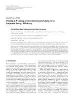
Figure 1: Demonstration of the cortical processing stage of the auditory model. The auditory spectrogram (left) is decomposed into its
spectrotemporal components using a bank of spectrotemporally selective filters. The impulse responses (spectrotemporal receptive fields
or STRF) of one such filters is shown in the center panels. The multiresolution (cortical) representation is computed by (2-dimensional)
convolution of the spectrogram with each STRF, generating a family of spectrograms with different spectral and temporal resolutions, that
is, the cortical representation is a 3-dimensional function of frequency, rate and scale (right cubes) that changes in time. A complete set of
STRFs guarantees an invertible map which is needed to reconstruct a spectrogram back from a modified cortical representation.
h
r
(·)(secondderivativeofaGaussianfunction)andh
s
(·)
(Gamma function), and their asymmetric Hilbert trans-
forms:
h
rate
(t; ω, θ) = h
r
(t; ω)cosθ +

h

r
(t; ω)sinθ,
h
scale
( f ; Ω, φ) = h
s
( f ; Ω)cosφ +

h
s
( f ; Ω)sinφ.
(4)
The impulse responses for different scales and rates are
given by dilation
h
r
(t; ω) = ωh
r
(ωt),
h
s
( f ; Ω) = Ωh
s
(Ω f ).
(5)
Therefore, the spectrotemporal response for an input spec-
trogram y(t, f )isgivenby
r
+
(t, f ; ω,Ω; θ,φ) = y(t, f )∗

t, f
STRF
+
(t, f ; ω,Ω; θ,φ),
r
−
(t, f ; ω,Ω; θ,φ) = y(t, f )∗
t, f
STRF
−
(t, f ; ω,Ω; θ,φ),
(6)
where
∗
tf
denotes convolution with respect to both t and f .
It is useful to compute the spectrotemporal response r
±
(·)
in terms of the output magnitude and phase of the down-
ward (+) and upward (
−) selective filters. For this, the tem-
poral and spatial filters, h
rate
and h
scale
,canbeequivalently
expressed in the wavelet-based analytical forms h
rw
(·)and

h
sw
(·)as
h
rw
(t; ω) = h
r
(t; ω)+j

h
r
(t; ω),
h
sw
( f ; Ω) = h
s
( f ; Ω)+j

h
s
( f ; Ω).
(7)
The complex response to downward and upward selective fil-
ters, z
+
(·)andz
−
(·), is then defined as
z
+

(t, f ; Ω, ω) = y(t, f )∗
tf

h
∗
rw
(t; ω)h
sw
( f ; Ω)

,
z
−
(t, f ; Ω, ω) = y(t, f )∗
tf

h
rw
(t; ω)h
sw
( f ; Ω)

,
(8)
where
∗ denotes the complex conjugate. The magnitude of
z
+
and z
−

is used throughout the paper as a measure of
speech and noise energy. The filters directly modify the mag-
nitude of z
+
and z
−
while keeping their phases unchanged.
The final view that emerges is that of a continuously updated
estimate of the spectral and temporal modulation content
of the auditory spectrogram Figure 1. All parameters of this
model are derived from physiological data in animals and
psychoacoustical data in human subjects as explained in de-
tail in [15–17].
Unlike conventional features, our auditory-based fea-
tures have multiple scales of time and spectral resolution.
Some respond to fast changes while others are tuned to
slower modulation patterns; a subset is selective to broad-
band spectra, and others are more narrowly tuned. For this
study, temporal filters (rate) ranging from 1 to 32 Hz and
spectral filters (scale) from 0.5 to 8.00 Cycle/Octave were
used to represent the spectrotemporal modulations of the
sound.
1.3. Reconstructing the sound from
the auditory representation
We resynthesize the sound from the output of cortical and
early auditory stages using a computational procedure de-
scribedindetailin[13]. While the nonlinear operations in
the early stage make it impossible to have perfect reconstruc-
tion, perceptually acceptable renditions are still feasible as
demonstrated in [13]. We obtain the reconstructed sound

from the auditory spectrogram using a method based on
the convex projection algorithm proposed in [12, 13]. How-
ever, the reconstruction of the auditory spectrogram from
the cortical representation (z
±
) is straightforward since it is
a linear transformation and can be easily inverted. In [13],
PESQ scores were derived to evaluate the quality of the re-
constructed speech from the cortical representation and the
typical score of 4+ was reported. In addition, subjective tests
were conducted to show that the reconstruction from the full
representation does not degrade the intelligibility [13].
4 EURASIP Journal on Audio, Speech, and Music Processing
1.4. Multiresolution representation of
speech and noise
In this section, we explain how the cortical representation
captures the modulation content of sound. We also demon-
strate the separation between representation of speech and
different kind of noise which is due to their distinct spec-
trotemporal patterns. The output of the cortical model de-
scribed in Section 1 is a 4-dimensional tensor with each point
indicating the amount of energy at corresponding time, fre-
quency, rate, and scale (z
±
(t, f , ω,Ω)). One can think of each
point in the spectrogram (e.g., time t
c
and frequency f
c
in

Figure 2) as having a two-dimensional rate-scale representa-
tion (z
± (t
c
, f
c
, ω, Ω)) that is an estimate of modulation en-
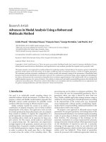
ergy at different temporal and spectral resolutions. The mod-
ulation filters with different resolutions capture local and
global information about each point as shown in Figure 2
for time t
c
and frequency f
c
of the speech spectrogram. In
this example, the temporal modulation has a peak around
4 Hz which is the typical temporal rate of speech. The spec-
tral modulation, scale, on the other hand spans a wide range
reflecting at its high end the harmonic structure due to voic-
ing (2–6 Cycle/Octave) and at its low end the spectral enve-
lope or formants (less than 2 Cycle/Octave). Another way of
looking at the modulation content of a sound is to collapse
the time dimension of the cortical representation resulting in
an estimate of the average rate-scale-frequency modulation
of the sound in that time window. This average is useful, es-
pecially when the sound is relatively stationary as is the case
for many background noises and is calculated in the follow-
ing way:
U
±

(ω, Ω, f ) =

t2
t1


z
±
(ω, Ω, f , t)


dt.
(9)
Figure 3 shows the average multiresolution representation
(U
±
from (9)) of speech and four different kinds of noise
chosen from Noisex database [18]. Top row of Figure 3 shows
the spectrogram of speech, white, jet, babble, and city noise.
These four kinds of noise are different in their frequency
distribution as well as in their spectrotemporal modulation
pattern as demonstrated in Figure 3.RowsB,C,andDin
Figure 3 show the average rate-scale, scale-frequency, and
rate-frequency representations of the corresponding sound
calculated from the average rate-scale-frequency representa-
tion (U
±
) by collapsing one dimension at a time. As shown
in rate-scale displays in Figure 3(b), speech has strong slow
temporal and low-scale modulation; on the other hand,

speech babble shows relatively faster temporal and higher
spectral modulation. Jet noise has a strong 10 Hz temporal
modulation which also has a high scale because of its narrow
spectrum. White noise has modulation energy spread over
a wide range of rates and scales. Figure 3(c) shows the av-
erage scale-frequency representation of the sounds, demon-
strating how the energy is distributed along the dimensions
of frequency and spectral modulation. Scale-frequency rep-
resentation shows a notable difference between speech and
babble noise with speech having stronger low-scale mod-
ulation energy. Finally, Figure 3(d) shows the average rate-
frequency representation of the sounds, that shows how en-
ergy is distributed in different frequency channels and tem-
poral rates. Again, jet noise shows a strong 10 Hz temporal
modulation at frequency 2 KHz. White noise on the other
hand activates most rate and frequency filters with increasing
energy for higher-frequency channels reflecting the increased
bandwidth of constant-Q auditory filters. Babble noise acti-
vates low and mid frequency filters better similar to speech
but at higher rates. City noise also activates wide range of
filters. As Figure 3 shows that spectrotemporal modulations
of speech have very different characteristics than the four
noises, which is the reason we can discriminately keep its
modulation components while reducing the noise ones. The
three-dimensional average noise modulation is what we used
as the noise model in the speech enhancement algorithm as
described in the next section.
1.5. Estimation of noise modulations
A crucial factor in affecting the performance of any noise
suppression technique is the quality of the background noise

estimation. In spectral subtraction algorithms, several tech-
niques have been proposed that are based on three assump-
tions: (1) speech and noise are statistically independent, (2)
speech is not always present, and (3) the noise is more sta-
tionary than speech [4]. One of these methods is voice activ-
ity detection (VAD) that estimates the likelihood of speech at
each time window and then uses the frames with low likeli-
hood of speech to update the noise model. One of the com-
mon problems with VADs is their poor performance at low
SNRs. To overcome this limitation, we employed a recently
formulated speech detector (also based on the cortical rep-
resentation) which detected speech reliably at SNR’s as low
as
−5dB [7]. In this method, the multiresolution represen-
tation of the incoming sound goes through a dimensionality
reduction algorithm based on tensor singular value decom-
position (TSVD [19]). This decomposition results in an ef-
fective reduction of redundant features in each of the sub-
spaces of rate, scale, and frequency resulting in a compact
representation that is suitable for classification. A trained
support vector machine (SVM [20]) uses this reduced rep-
resentation to estimate the likelihood of speech at each time
frame. The SVM is trained independently on clean speech
and nonspeech samples and has been shown to generalize
well to novel examples of speech in noise at low SNR, and
hence is amenable for real-time implementation [7]. The
frames marked by the SVM as nonspeech are then added to
the noise model (N
±
),whichisanestimateofnoiseenergyat

each frequency, rate, and scale:
N
±
( f , ω, Ω) =

noise frames


z
±
(t, f , ω,Ω)


dt.
(10)
As shown in Figure 3, this representation is able to capture
the noise information beyond just the frequency distribu-
tion, as is the case with most spectral subtraction-based ap-
proaches. Also, as can be seen in Figure 3, speech and most
kinds of noises are well separated in this domain.
N. Mesgarani and S. Shamma 5
0.25
0.5
1
f
c
4
0 t
c
1.3s

Time
Ω (cyc/oct)
Frequency (KHz)
Auditory spectrogram
|z(t
c
, f
c
, ω, Ω)|
-
+
8
0.5
−32 −40 432
ω (Hz)
01
Normalized energy
Figure 2: Rate-scale representation of clean speech. Spectrotemporal modulations of speech are estimated by a bank of modulation selective
filters, and are depicted at a particular time instant and frequency t
c
and f
c
) by the 2-dimensional distribution on the right.
0.25
0.5
1
2
4
0.21.4
Time (s)

Frequency (KHz)
Speech
0.25
0.5
1
2
4
0.21.4
Time (s)
White
0.25
0.5
1
2
4
0.21.4
Time (s)
Jet
0.25
0.5
1
2
4
0.21.4
Time (s)
Babble
0.25
0.5
1
2

4
0.21.4
Time (s)
City
(a)
0.5
1
2
4
−32 −8 −11 8 32
Rate (Hz)
Scale (cyc/oct)
0.5
1
2
4
−32 −8 −11 8 32
Rate (Hz)
0.5
1
2
4
−32 −8 −11 8 32
Rate (Hz)
0.5
1
2
4
−32 −8 −11 8 32
Rate (Hz)

0
1
0.5
1
2
4
−32 −8 −11 8 32
Rate (Hz)
Normalized energy
(b)
0.5
1
2
4
0.25 0.51 2 4
Frequency (KHz)
Scale (cyc/oct)
0.5
1
2
4
0.25 0.51 2 4
Frequency (KHz)
0.5
1
2
4
0.25 0.51 2 4
Frequency (KHz)
0.5

1
2
4
0.25 0.51 2 4
Frequency (KHz)
0.5
1
2
4
0.25 0.51 2 4
Frequency (KHz)
Normalized energy
0
1
(c)
0.25
0.5
1
2
4
−32 −8 −11 8 32
Rate (Hz)
Frequency (KHz)
0.25
0.5
1
2
4
−32 −8 −11 8 32
Rate (Hz)

0.25
0.5
1
2
4
−32 −8 −11 8 32
Rate (Hz)
0.25
0.5
1
2
4
−32 −8 −11 8 32
Rate (Hz)
0.25
0.5
1
2
4
−32 −8 −11 8 32
Rate (Hz)
(d)
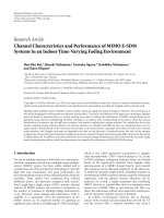
Figure 3: Auditory spectrogram and average cortical representations of speech and four different kinds of noise. Row (a): auditory spec-
trogram of speech, white, jet, babble, and city noise taken from Noisex database. Row (b): average rate-scale representations of sound
demonstrate the distribution of energy in different temporal and spectral modulation filters. Speech is well separated from the noises in this
representation. Row (c): average scale-frequency representations. jet have mostly high scales because of its narrow-band frequency distribu-
tions. Row (d): average rate-frequency representations show the energy distributions in different frequency channels and rate filters.
6 EURASIP Journal on Audio, Speech, and Music Processing
0.25
0.5

1
f
c
4
0 t
c
1.3s
Time
Frequency (KHz)
Auditory spectrogram
S
N
(t
c
, f
c
, ω, Ω)
-
+
N(t
c
, f
c
, ω, Ω)
-
+
H(t
c
, f
c

, ω, Ω)
-
+
Ω
8
2
0.5
8
2
0.5
−10 −40 410Hz
8
0.5
ω
01
Normalized energy
−10 −40410Hz
A
B
C
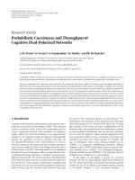
Figure 4: Filtering the rate-scale representation: modulations due to the noise are filtered out by weighting the rate-scale representation
of noisy speech with the function H(t, f , ω, Ω). In this example, the jet one noise from Noisex was added to clean speech at SNR 10 dB.
The rate-scale representation of the signal, r
s
(t
c
, f
c
, ω, Ω) and the rate-scale representation of noise, N(t
c

, f
c
, ω, Ω)wereusedtoobtainthe
necessary weighting as a function of ω and Ω (11). This weighting was applied to the rate-scale representation of the signal, r
s
(t
c
, f
c
, ω, Ω)
to restore modulations typical of clean speech. The restored modulation coefficients were then used to reconstruct the cleaned auditory
spectrogram, and from it the corresponding audio signal.
0.25
0.5
1
2
4
Frequency (KHz)
12 dB
0.25
0.5
1
2
4
Frequency (KHz)
6dB
0.25
0.5
1
2

4
03
Time (s)
Frequency (KHz)
0dB
Original
Cleaned
Jet noise
03
Time (s)
01
Normalized energy
Figure 5: Examples of restored spectrograms after “filtering” of
spectrotemporal modulations. Jet noise from Noisex was added to
speech at SNRs 12 dB (top), 6 dB (middle) and 0 dB (bottom) pan-
els. Left panels show the original noisy speech and right panels show
the denoised ones. The clean speech spectrum has been restored al-
though the noise has a strong temporally modulated tone (10 Hz)
mixed in with the speech signal near 2 kHz (indicated by the arrow).
2. NOISE SUPPRESSION
The exact rule for suppressing noise coefficients is a deter-
mining factor in the subjective quality of the reconstructed
enhanced speech, especially with regards to the reduction of
musical noise [4]. Having the spectrotemporal representa-
tion of noisy sound and the model of noise average modu-
lation energy, one can design a rule that suppresses the mod-
ulations activated by the noise and emphasize the ones that
are from the speech signal. One possible way of doing this is
to use a Wiener filter in the following form:
H

±
(t, f , ω,Ω) =

SNR
±
(t, f , ω,Ω)
1+SNR
±
(t, f , ω,Ω)

≈

1 −
N
±
( f , ω, Ω)
S
N±
(t, f , ω,Ω)

,
(11)
where N
±
is our noise model calculated by averaging the cor-
tical representation of noise-only frames (10)andS
N
is the
cortical representation of noisy speech signal. The resulting
gain function (11) maintain the output of filters with high

SNR values while attenuating the output of low-SNR filters:
z
±
(t, f , ω,Ω) = z
±
(t, f , ω,Ω)·H
±
(t, f , ω,Ω),
(12)
z is the modified (denoised) cortical representation from
which the cleaned speech is reconstructed. This idea is
demonstrated in Figure 4. Figure 4A shows the spectrogram
of a speech sample contaminated by jet noise and its rate-
scale representation at time t
c
and frequency f
c
(Figure 4A)
which is a point in the spectrogram that noise and speech
overlap. As discussed in Section 1.4, this type of noise has
a strong temporally modulated tone (10 Hz) at frequency
around 2 KHz. The rate-scale representation of the jet noise
for the same frequency, f
c
, is shown in Figure 4B. Com-
paring the noisy speech representation with the one from
N. Mesgarani and S. Shamma 7
White
2
3

Subjective MOS
0612
SNR (dB)
Modulation
Wiener
Original
Jet
2
3
0612
SNR (dB)
Modulation
Wiener
Original
Babble
2
3
0612
SNR (dB)
Modulation
Wiener
Original
City
2
3
0612
SNR (dB)
Modulation
Wiener
Original

(a)
2
3
Objective PESQ score
0612
SNR (dB)
Modulation
Wiener
Original
2
3
0612
SNR (dB)
Modulation
Wiener
Original
2
3
0612
SNR (dB)
Modulation
Wiener
Original
2
3
0612
SNR (dB)
Modulation
Wiener
Original

(b)
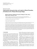
Figure 6: Subjective and objective scores on a scale of 1 to 5 for degraded and denoised speech using modulation and Wiener methods.
(a): Subjective MOS scores and errorbars averaged over ten subjects for white, jet, babble, and city noise. (b): Objective scores and errorbars
transformed to a scale of 1 to 5 for degraded and denoised speech using modulation and Wiener methods.
noise model, it is easy to see what parts belong to noise
and what parts come from the speech signal. Therefore, we
can recover the clean rate-scale representation by attenuat-
ing the modulation rates and scales that show strong en-
ergy in the noise model. This intuitive idea is performed by
formula (11) which for this example results in the function
shown in Figure 4C. The H function has low gain for fast
modulation rates and high scales that are due to the back-
ground noise (as shown in Figure 4B), while emphasizing the
slow modulations (<5 Hz) and low scales (<2 cyc/oct) that
come mostly from speech signal. Multiplication of this rate-
scale-frequency gain which is a function of time, and the
noisy speech representation results in denoised representa-
tion which is then used to reconstruct the spectrogram of the
cleaned speech signal using the inverse cortical transforma-
tion (Figure 5).
3. RESULTS FROM EXPERIMENTAL EVALUATIONS
To examine the effectiveness of the noise suppression algo-
rithm, we used subjective and objective tests to compare the
quality of denoised signal with the original and a Wiener fil-
ter noise suppression method by Scalart and Filho [21]im-
plemented in [22]. The noisy speech sentences were gener-
ated by adding four different kinds of noise: white, jet, bab-
ble, and city from Noisex [18] to eight clean speech samples
from TIMIT [23]. The test material was prepared at three
SNR values: 0, 6, and 12 dB. We used mean opinion score

(MOS) test to evaluate the subjective quality of the denoising
algorithm. In the subjective quality tests, ten subjects were
asked to score the quality of the original and denoised speech
samples between one (bad) and five (excellent). All sub-
jects had prior experience in psychoacoustics experiments
and had self-reported normal hearing. The sounds were pre-
sented in a quiet room over headphones at a comfortable lis-
tening level (approximately 70 dB) and the responses were
collected using a computer interface. Figure 6(a) shows the
MOS score and the errorbars for the original and denoised
signals using modulation and Wiener methods. The results
are shown for four types of noise and three SNR levels. In
most stationary noise conditions, subjects reported the high-
est scores for the modulation method. However, for the non-
stationary sounds, the modulation method outperformed
the Wiener methods in the babble tests, and produced com-
parable results for the city sounds. In addition, we conducted
objective test using perceptual evaluation of speech quality
(PESQ) [24] measure for the twelve conditions to obtain
the objective score for each sample. The resulting scores and
their errorbars are reported in Figure 6(b).PESQgiveshigher
score for the modulation method in the stationary condi-
tions, but the performance in this measure appears compara-
ble for the nonstationary conditions. Our method performs
better for stationary noise because of its ability to model the
average spectrotemporal properties of the stationary noise
8 EURASIP Journal on Audio, Speech, and Music Processing
better. This also explains the better performance in the bab-
ble speech since the babble is relatively “stationary” in its
long-term spectrotemporal behavior, especially compared to

the city noise which fluctuates considerably.
4. CONCLUSIONS
We have described a new approach for the denoising of con-
taminated broadband complex signals such as speech. In this
method, the noisy signal is first transformed to the spec-
trotemporal modulation domain in which the speech and
noise are separated based on their distinct modulation pat-
terns. This allows for the possibility of suppressing noise even
when it spectrally overlaps with the desired signal. The spec-
trotemporal representation used is based on a model of audi-
tory processing [13] inspired by physiological data from the
mammalian primary auditory cortex. Subjective and objec-
tive tests are reported that they demonstrate the effectiveness
of this method in enhancing the quality of speech without
introducing artifacts or substantially deleting spectrally over-
lapping speech energy.
ACKNOWLEDGMENTS
The authors wish to thank Telluride Neuromorphic Engi-
neering Workshop. Partial funding for this project was ob-
tained from the Air Force Office of Scientific Research, and
the National Science Foundation (ITR, 1150086075). We also
acknowledge support through the NIH R01 DC005779.
REFERENCES
[1] J. S. Lim and A. V. Oppenheim, “Enhancement and bandwith
compression of noisy speech,” Proceedings of the IEEE, vol. 67,
no. 12, pp. 1586–1604, 1979.
[2] Y. Ephraim and H. L. Van Trees, “Signal subspace approach for
speech enhancement,” IEEE Transactions on Speech and Audio
Processing, vol. 3, no. 4, pp. 251–266, 1995.
[3] Y. Ephraim and D. Malah, “Speech enhancement using a min-

imum mean-square error-log-spectral amplitude estimator,”
IEEE Transactions on Acoustics, Speech, and Sig nal Processing,
vol. 33, no. 2, pp. 443–445, 1985.
[4] R. Martin, “Statistical methods for the enhancement of noisy
speech,” in Proceedings of the 8th IEEE International Workshop
on Acoustic Echo and Noise Control (IWAENC ’03), pp. 1–6,
Kyoto, Japan, September 2003.
[5] S. Shamma, “Encoding sound timbre in the auditory system,”
IETE Journal of Research, vol. 49, no. 2, pp. 193–205, 2003.
[6] M. Elhilali, T. Chi, and S. Shamma, “A spectro-temporal mod-
ulation index (STMI) for assessment of speech intelligibility,”
Speech Communication, vol. 41, no. 2-3, pp. 331–348, 2003.
[7] N. Mesgarani, S. Shamma, and M. Slaney, “Speech discrim-
ination based on multiscale spectro-temporal modulations,”
in Proceedings of IEEE International Conference on Acoustics,
Speech and Signal Processing (ICASSP ’04), vol. 1, pp. 601–604,
Montreal, Canada, May 2004.
[8] R. P. Carlyon and S. Shamma, “An account of monaural
phase sensitivity,” JournaloftheAcousticalSocietyofAmerica,
vol. 114, no. 1, pp. 333–348, 2003.
[9] J. Tchroz and B. Kollmeier, “SNR estimation based on am-
plitude modulation analysis with applications to noise sup-
pression,” IEEE Transactions on Speech and Audio Processing,
vol. 11, no. 3, pp. 184–192, 2003.
[10] K. Wang and S. Shamma, “Spectral shape analysis in the cen-
tral auditory system,” IEEE Transactions on Speech and Audio
Processing, vol. 3, no. 5, pp. 382–395, 1995.
[11] R. Lyon and S. Shamma, “Auditory representation of timbre
and pitch,” in Auditory Computation, vol. 6 of Springer Hand-
book of Auditory Research, pp. 221–270, Springer, New York,

NY, USA, 1996.
[12] X. Yang, K. Wang, and S. Shamma, “Auditory representations
of acoustic signals,” IEEE Transactions on Information The-
ory, vol. 38, no. 2, part 2, pp. 824–839, 1992, special issue on
wavelet transforms and multi-resolution signal analysis.
[13] T. Chi, P. Ru, and S. Shamma, “Multiresolution spectrotempo-
ral analysis of complex sounds,” Journal of the Acoustical Soci-
ety of America, vol. 118, no. 2, pp. 887–906, 2005.
[14] S. Shamma, “Methods of neuronal modeling,” in Spatial and
Temporal Processing in the Auditory System, pp. 411–460, MIT
press, Cambridge, Mass, USA, 2nd edition, 1998.
[15] D. A. Depireux, J. Z. Simon, D. J. Klein, and S. Shamma,
“Spectro-temporal response field characterization with dy-
namic ripples in ferret primary auditory cortex,” Journal of
Neurophysiology, vol. 85, no. 3, pp. 1220–1234, 2001.
[16] N. Kowalski, D. A. Depireux, and S. Shamma, “Analysis of dy-
namic spectra in ferret primary auditory cortex. I. Character-
istics of single-unit responses to moving ripple spectra,” Jour-
nal of Neurophysiology, vol. 76, no. 5, pp. 3503–3523, 1996.
[17] M. Elhilali, T. Chi, and S. Shamma, “A spectro-temporal mod-
ulation index (STMI) for assessment of speech intelligibility,”
Speech Communication, vol. 41, no. 2-3, pp. 331–348, 2003.
[18] A. Varga, H. J. M. Steeneken, M. Tomlinson, and D. Jones,
“The NOISEX-92 study on the effect of additive noise on au-
tomatic speech recognition,” Documentation included in the
NOISEX-92 CD-ROMs, 1992.
[19] L. De Lathauwer, B. De Moor, and J. Vandewalle, “A multi-
linear singular value decomposition,” SIAM Journal on Matrix
Analysis and Applications, vol. 21, no. 4, pp. 1253–1278, 2000.
[20] V. N. Vapnik,

The Nature of Statistical Learning Theory,
Springer, Berlin, Germany, 1995.
[21] P. Scalart and J. V. Filho, “Speech enhancement based on a pri-
ori signal to noise estimation,” in Proceedings of IEEE Inter-
national Conference on Acoustics, Speech and Signal Processing
(ICASSP ’96), vol. 2, pp. 629–632, Atlanta, Ga, USA, May 1996.
[22] E. Zavarehei, />Esfandiar.
[23] S. Seneff and V. Zue, “Transcription and alignment of the
timit database,” in An Acoustic Phonetic Continuous Speech
Database, J. S. Garofolo, Ed., National Institute of Standards
and Technology (NIST), Gaithersburgh, Md, USA, 1988.
[24] “Perceptual evaluation of speech quality (PESQ): an objective
method for end-to-end speech quality assessment of narrow-
band telephone networks and speech codecs,” ITU-T Recom-
mendation P.862, February 2001.