Báo cáo hóa học: "Research Article Activity Representation Using 3D Shape Models" pot

Hindawi Publishing Corporation
EURASIP Journal on Image and Video Processing
Volume 2008, Article ID 347050, 16 pages
doi:10.1155/2008/347050
Research Article
Activity Representation Using 3D Shape Models
Mohamed F. Abdelkader,
1
Amit K. Roy-Chowdhury,
2
Rama Chellappa,
1
and Umut Akdemir
3
1
Department of Electrical and Computer Engineering and Center for Automation Research, UMIACS, University of Maryland,
College Park, MD 20742, USA
2
Department of Electrical Engineering, University of California, Riverside, CA 92521, USA
3
Siemens Corporate Research, Princeton, NJ 08540, USA
Correspondence should be addressed to Mohamed F. Abdelkader,
Received 1 February 2007; Revised 9 July 2007; Accepted 25 November 2007
Recommended by Maja Pantic
We present a method for characterizing human activities using 3D deformable shape models. The motion trajectories of points
extracted from objects involved in the activity are used to build models for each activity, and these models are used for classification
and detection of unusual activities. The deformable models are learnt using the factorization theorem for nonrigid 3D models.
We present a theory for characterizing the degree of deformation in the 3D models from a sequence of tracked observations. This
degree, termed as deformation index (DI), is used as an input to the 3D model estimation process. We study the special case of
ground plane activities in detail because of its importance in video surveillance applications. We present results of our activity
modeling approach using videos of both high-resolution single individual activities and ground plane surveillance activities.

Copyright © 2008 Mohamed F. Abdelkader et al. This is an open access article distributed under the Creative Commons
Attribution License, which permits unrestricted use, distribution, and reproduction in any medium, provided the original work is
properly cited.
1. INTRODUCTION
Activity modeling and recognition from video is an impor-
tant problem, with many applications in video surveillance
and monitoring, human-computer interaction, computer
graphics, and virtual reality. In many situations, the problem
of activity modeling is associated with modeling a represen-
tative shape which contains significant information about
the underlying activity. This can range from the shape of the
silhouette of a person performing an action to the trajectory
of the person or a part of his body. However, these shapes
are often hard to model because of their deformability and
variations under different camera viewing directions.
In all of these situations, shape theory provides powerful
methods for representing these shapes [1, 2]. The work in
this area is divided between 2D and 3D deformable shape
representations. The 2D shape models focus on comparing
the similarities between two or more 2D shapes [2–6]. Two-
dimensional representations are usually computationally
efficient and there exists a rich mathematical theory using
which appropriate algorithms could be designed. Three-
dimensional models have received much attention in the
past few years. In addition to the higher accuracy provided
by these methods, they have the advantage that they can
potentially handle variations in camera viewpoint. However,
the use of 3D shapes for activity recognition has been much
less studied. In many of the 3D approaches, a 2D shape is
represented by a finite-dimensional linear combination of

3D basis shapes and a camera projection model relating the
3D and 2D representations [7–10]. This method has been
applied primarily to deformable object modeling and track-
ing. In [11], actions under different variability factors were
modeled as a linear combination of spatiotemporal basis
actions. The recognition in this case was performed using
the angles between the action subspaces without explicitly
recovering the 3D shape. However, this approach needs
sufficient video sequences of the actions under different
viewing directions and other forms of variability to learn the
space of each action.
1.1. Major contributions of the paper
In this paper, we propose an approach for activity rep-
resentation and recognition based on 3D shapes gener-
ated by the activity. We use the 3D deformable shape
model for characterizing the objects corresponding to each
activity. The underlying hypothesis is that an activity can
be represented by deformable shape models that capture
2 EURASIP Journal on Image and Video Processing
the 3D configuration and dynamics of the set of points
taking part in the activity. This approach is suitable for
representing different activities as shown by experiments in
Section 5. This idea has also been used for 2D shape-based
representation in [12, 13]. We also propose a method for
estimating the amount of deformation of a shape sequence
by deriving a “deformability index” (DI). Estimation of the
DI is noniterative, does not require selecting an arbitrary
threshold, and can be done before estimating the 3D
structure, which means that we can use it as an input
to the 3D nonrigid model estimation process. We study

the special case of ground plane activities in more detail
as an important application because of its importance in
surveillance scenarios. The 3D shapes in this special scenario
are constrained by the ground plane which reduces the
problem to a 2D shape representation. Our method in this
case has the ability to match the trajectories across different
camera viewpoints (which would not be possible using 2D
shape modeling methods) and the ability to estimate the
number of activities using the DI formulation. Preliminary
versions of this work appeared in [14, 15]andamoredetailed
analysis of the concept of measuring the deformability was
presented in [16].
We have tested our approach on different experimental
datasets. First we validate our DI estimate using motion
capturedataaswellasvideosofdifferent human activities.
The results show that the DI is in accordance with our
intuitive judgment and corroborates certain hypotheses
prevailing in human movement analysis studies. Subse-
quently, we present the results of applying our algorithm
to two different applications: view-invariant human activity
recognition using 3D models (high-resolution imaging) and
detection of anomalies in ground plane surveillance scenario
(low-resolution imaging).
The paper is organized as follows. Section 2 reviews some
of the existing work in event representation and 3D shape
theory. Section 3 describes the shape-based activity modeling
approach along with the special case of ground plane motion
trajectories. Section 4 presents the method for estimating the
DI for a shape sequence. Detailed experiments are presented
in Section 5, before concluding in Section 6.

2. RELATED WORK
Activity representation and recognition have been an active
area of research for decades and it is impossible to do justice
to the various approaches within the scope of this paper. We
outline some of the broad trends in this area. Most of the
early work on activity representation comes from the field of
artificial intelligence (AI) [17, 18]. More recent work comes
from the fields of image understanding and visual surveil-
lance, employing formalisms like hidden Markov models
(HMMs), logic programming, and stochastic grammars [19–
29]. A method for visual surveillance using a “forest of
sensors” was proposed in [30]. Many uncertainty-reasoning
models have been actively pursued in the AI and image
understanding literature, including belief networks [31–33],
Dempster-Shafer theory [34], dynamic Bayesian networks
[35, 36], and Bayesian inference [37]. A specific area of
research within the broad domain of activity recognition is
human motion modeling and analysis, which has received
keen interest from various disciplines [38–40]. A survey of
some of the earlier methods used in vision for tracking
human movement can be found in [41], while a more recent
survey is in [42].
The use of shape analysis for activity and action recog-
nition has been a recent trend in the literature. Kendall’s
statistical shape theory was used to model the interactions
of a group of people and objects in [43], as well as the
motion of individuals [44]. A method for the representation
of human activities based on space curves of joint angles and
torsolocationandattitudewasproposedin[45]. In [46],
the authors proposed an activity recognition algorithm using

dynamic instants and intervals as view-invariant features,
and the final matching of trajectories was conducted using
a rank constraint on the 2D shapes. In [47], each human
action was represented by a set of 3D curves which are
quasi-invariant to the viewing direction. In [48, 49], the
motion trajectories of an object are described as a sequence
of flow vectors, and neural networks are used to learn the
distribution of these sequences. In [50], a wavelet transform
was used to decompose the raw trajectory into components
of different scales, and the different subtrajectories are
matched against a data base to recognize the activity.
In the domain of 3D shape representation, the approach
of approximating a nonrigid object by a composition of basis
shapes has been useful in certain problems related to object
modeling [51]. However, there has been little analysis of its
usefulness in activity modeling, which is the focus of this
paper.
3. SHAPE-BASED ACTIVITY MODELS
3.1. Motivation
We propose a framework for recognizing activities by first
extracting the trajectories of the various points taking part
in the activity, followed by a nonrigid 3D shape model fitted
to the trajectories. It is based on the empirical observation
that many activities have an associated structure and a
dynamical model. Consider, as an example, the set of images
of a walking person in Figure 1(a) (obtained from the USF
database for the gait challenge problem [52]). The binary
representation clearly shows the change in the shape of the
body for one complete walk cycle. The person in this figure
is free to move his/her hands and feet any way he/she likes.

However, this random movement does not constitute the
activity of walking. For humans to perceive and appreciate
the walk, the different parts of the body have to move in a
certain synchronized manner. In mathematical terms, this is
equivalent to modeling the walk by the deformations in the
shape of the body of the person. Similar observations can be
made for other activities performed by a single human, for
example, dancing, jogging, sitting, and so forth.
An analogous example can be provided for an activity
involving a group of people. Consider people getting off
a plane and walking to the terminal, where there is no
jet-bridge to constrain the path of the passengers (see
Mohamed F. Abdelkader et al. 3
(a) (b)
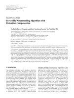
Figure 1: Two examples of activities: (a) the binary silhouette of a walking person and (b) people disembarking from an airplane. It is clear
that both of these activities can be represented by deformable shape models using the body contour in (a) and the passenger/vehicle motion
paths in (b).
Figure 1(b)). Every person after disembarking is free to move
as he/she likes. However, this does not constitute the activity
of people getting off a plane and heading to the terminal.
The activity here is comprised of people walking along a
path that leads to the terminal. Again, we see that the activity
can be modeled by the shape of the trajectories taken by the
passengers. Using deformable shape models is a higher-level
abstraction of the individual trajectories, and it provides a
method of analyzing all the points of interest together, thus
modeling their interactions in a very elegant way.
Not only is the activity represented by a deformable shape
sequence, but also the amount of deformation is different for
different activities. For example, it is reasonable to say that

the shape of the human body while dancing is usually more
deformable than during walking, which is more deformable
than when standing still. Since it is possible for the human
observer to roughly infer the degree of deformability based
on the contents of the video sequence, the information
about how deformable a shape is must be contained in the
sequence itself. We will use this intuitive notion to quantify
the deformability of a shape sequence from a set of tracked
points on the object. In our activity representation model,
a deformable shape is represented as a linear combination
of rigid basis shapes [7]. The deformability index provides a
theoretical framework for estimating the required number of
basis shapes.
3.2. Estimation of deformable shape models
We hypothesize that each shape sequence can be represented
by a linear combination of 3D basis shapes. Mathematically,
if we consider the trajectories of P points representing the
shape (e.g., landmark points), then the overall configuration
of the P points is represented as a linear combination of the
basis shapes S
i
as
S
=
K

i=1
l
i
S

i
, S, S
i
∈ R
3×P
, l ∈ R,(1)
where l
i
represents the weight associated with the basis shape
S
i
.
ThechoiceofK is determined by quantifying the
deformability of the shape sequence, and it will be studied
in detail in Section 4.Wewillassumeaweakperspective
projection model for the camera.
A number of methods exist in the computer vision
literature for estimating the basis shapes. In the factorization
paper for structure from motion [53], the authors considered
P points tracked across F framesinordertoobtaintwo
F
× P matrices, that is, U and V.EachrowofU contains
the x-displacements of all the P points for a specific time
frame, and each row of V contains the corresponding y-
displacements. It was shown in [53] that for 3D rigid motion
and the orthographic camera model, the rank r of the
concatenation of the rows of the two matrices [U/V]has
an upper bound of 3. The rank constraint is derived from
the fact that [U/V] can be factored into two matrices, M
2F×r

and S
r×P
, corresponding to the pose and 3D structure of the
scene, respectively. In [7], it was shown that for nonrigid
motion, the above method could be extended to obtain a
similar rank constraint, but one that is higher than the bound
for the rigid case. We will adopt the method suggested in
[7] for computing the basis shapes for each activity. We will
outline the basic steps of their approach in order to clarify
the notation for the remainder of the paper.
Given F frames of a video sequence with P moving
points, we first obtain the trajectories of all these points over
the entire video sequence. These P points can be represented
in a measurement matrix as
W
2F×P
=
⎡
⎢
⎢
⎢
⎢
⎢
⎢
⎢
⎢
⎣
u
1,1
··· u

1,P
v
1,1
··· v
1,P
.
.
.
.
.
.
.
.
.
u
F,1
··· u
F,P
v
F,1
··· v
F,P
⎤
⎥
⎥
⎥
⎥
⎥
⎥
⎥

⎥
⎦
,(2)
4 EURASIP Journal on Image and Video Processing
where u
f ,p
represents the x-position of the pth point in the
f th frame and v
f ,p
represents the y-position of the same
point. Under weak perspective projection, the P points of
aconfigurationinaframe f are projected onto 2D image
points (u
f ,i
, v
f ,i
)as

u
f ,1
··· u
f ,P
v
f ,1
··· v
f ,P

=
R
f


K

i=1
l
f ,i
S
i

+ T
f
,(3)
where
R
f
=

r
f 1
r
f 2
r
f 3
r
f 4
r
f 5
r
f 6


Δ
=
⎡
⎣
R
(1)
f
R
(2)
f
⎤
⎦
. (4)
R
f
represents the first two rows of the full 3D camera
rotation matrix and T
f
is the camera translation. The
translation component can be eliminated by subtracting
out the mean of all the 2D points, as in [53]. We now
form the measurement matrix W, which was represented
in (2), with the means of each of the rows subtracted. The
weak perspective scaling factor is implicitly coded in the
configuration weights
{l
f ,i
}.
Using (2)and(3), it is easy to show that
W

=
⎡
⎢
⎢
⎢
⎢
⎢
⎣
l
1,1
R
1
··· l
1,K
R
1
l
2,1
R
2
··· l
2,K
R
2
.
.
.
.
.
.

.
.
.
l
F,1
R
F
··· l
F,K
R
F
⎤
⎥
⎥
⎥
⎥
⎥
⎦
⎡
⎢
⎢
⎢
⎢
⎢
⎣
S
1
S
2
.

.
.
S
K
⎤
⎥
⎥
⎥
⎥
⎥
⎦
=
Q
2F×3K
·B
3K×P
,(5)
which is of rank 3K.ThematrixQ contains the pose for
each frame of the video sequence and the weights l
1
, , l
K
.
The matrix B contains the basis shapes corresponding to
each of the activities. In [7], it was shown that Q and
B can be obtained by using singular value decomposition
(SVD) and retaining the top 3K singular values, as W
2F×P
=
UDV

T
and Q = UD
1/2
and B = D
1/2
V
T
. The solution is
unique up to an invertible transformation. Methods have
been proposed for obtaining an invertible solution using
the physical constraints of the problem. This has been dealt
with in detail in previous papers [9, 51]. Although this is
important for implementing the method, we will not dwell
on it in detail in this paper and will refer the reader to
previous work.
3.3. Special case: ground plane activities
A special case of activity modeling that often occurs is the
case of ground plane activities, which are often encoun-
tered in applications such as visual surveillance. In these
applications, the objects are far away from the camera such
that each object can be considered as a point moving on
a common plane such as the ground plane of the scene
under consideration. Because of the importance of such
configurations, we study them in more detail and present
an approach for using our shape-based activity model to
π
x
y
z
x

X
π
C
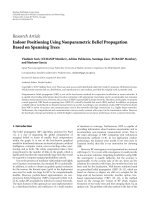
Figure 2: Perspective images of points in a plane [57]. The world
coordinate system is moved in order to be aligned with the plane π.
represent these ground plane activities. The 3D shapes in
this case are reduced to 2D shapes due to the ground plane
constraint. The main reason for using our 3D approach (as
opposed to a 2D shape matching one) is the ability to match
the trajectories across changes of viewpoint.
Our approach for this situation consists of two steps. The
first step recovers the ground plane geometry and uses it to
remove the projection effects between the trajectories that
correspond to the same activity. The second step uses the
deformable shape-based activity modeling technique to learn
a nominal trajectory that represents all the ground plane
trajectories generated by an activity. Since each activity can
be represented by one nominal trajectory, we will not need
multiple basis shapes for each activity.
3.3.1. First step: ground plane calibration
Most of the outdoor surveillance systems monitor a ground
plane of an area of interest. This area could be the floor
of a parking lot, the ground plane of an airport, or any
other monitored area. Most of the objects being tracked and
monitored are moving on this dominant plane. We use this
fact to remove the camera projection effect by recovering
the ground plane and projecting all the motion trajectories
back onto this ground plane. In other words, we map the
motion trajectories measured at the image plane onto the
ground plane coordinates to remove these projective effects.

Many automatic or semiautomatic methods are available to
perform this calibration [54, 55]. As the calibration process
needs to be performed only one time because the camera is
fixed, we are using the semiautomatic method presented in
[56], which is based on using some of the features often seen
in man-made environments. We will give a brief summary of
this method for completeness.
Consider the case of points lying on a world plane π,
as shown in Figure 2. The mapping between points X
π
=
(X, Y,1)
T
on the world plane π and their image x is a
general planar homography—a plane-to-plane projective
transformation—of the form x
= HX
π
,withH being a
3
× 3 matrix of rank 3. This projective transformation can
be decomposed into a chain of more specialized transforma-
tions of the form
H
= H
S
H
A
H
P

,(6)
where H
S
, H
A
,andH
P
represent similarity, affine, and pure
projective transformations, respectively. The recovery of the
ground plane up to a similarity is performed in two stages.
Mohamed F. Abdelkader et al. 5
Stage1:fromprojectivetoaffine
This is achieved by determining the pure projective transfor-
mation matrix H
P
. We note that the inverse of this projective
transformation is also a projective transformation

H
P
,which
can be written as

H
P
=
⎡
⎢
⎣
100

010
l
1
l
2
l
3
⎤
⎥
⎦
,(7)
where l
∞
= (l
1
, l
2
, l
3
)
T
is the vanishing line of the plane,
defined as the line connecting all the vanishing points for
lines lying on the plane.
From (7), it is evident that identifying the vanishing
line is enough to remove the pure projective part of the
projection. In order to identify the vanishing line, two sets
of parallel lines should be identified. Parallel lines are easy
to find in man-made environments (e.g., parking space
markers, curbs, and road lanes).

Stage 2: from affine to metric
The second stage of the rectification is the removal of the
affine projection. As in the first stage, the inverse affine
transformation matrix

H
A
can be written in the following
form:

H
A
=
⎡
⎢
⎢
⎢
⎢
⎣
1
β
−
α
β
0
010
001
⎤
⎥
⎥

⎥
⎥
⎦
. (8)
Also, this matrix has two degrees of freedom represented by α
and β. These two parameters have a geometric interpretation
as representing the circular points, which are a pair of points
at infinity that are invariant to Euclidean transformations.
Once these points are identified, metric properties of the
plane are available.
Identifying two affine invariant properties on the ground
plane can be sufficient to obtain two constraints on the values
of α and β. Each of these constraints is in the form of a circle.
These properties include a known angle between two lines,
equality of two unknown angles, and a known length ratio of
two line segments.
3.3.2. Second step: learning trajectories
After recovering the ground plane (i.e., finding the projective

H
P
and affine

H
A
inverse transformations), the motion tra-
jectories of the objects are reprojected to their ground plane
coordinates. Having m different trajectories of each activity,
the goal is to obtain a nominal trajectory that represents all
of these trajectories. We assume that all these trajectories

have the same 2D shape up to a similarity transformation
(translation, rotation, and scale). This transformation will
compensate for the way the activity was performed in the
scene. We use the factorization algorithm to obtain the shape
of this nominal trajectory from all the motion trajectories.
For a certain activity that we wish to learn, let T
j
be the
jth ground plane trajectory of this activity. This trajectory
was obtained by tracking an object performing the activity in
the image plane over n frames and by projecting these points
onto the ground plane as
T
j
=
⎡
⎢
⎢
⎣
x
j1
··· x
jn
y
j1
··· y
jn
1 ··· 1
⎤
⎥

⎥
⎦
=

H
A

H
P
⎡
⎢
⎢
⎣
u
j1
··· u
jn
v
j1
··· v
jn
1 ··· 1
⎤
⎥
⎥
⎦
,(9)
where u, v are the 2D image plane coordinates, x, y are the
ground plane coordinates, and


H
P
and

H
A
are the pure
projective and affine transformations from image to ground
planes, respectively.
Assume, except for a noise term η
j
, that all the different
trajectories correspond to the same 2D nominal trajectory
S but have undergone 2D similarity transformations (scale,
rotation, and translation). Then
T
j
= H
Sj
S + η
j
=
⎡
⎢
⎢
⎣
s
j
cos θ
j

−s
j
sin θ
j
t
xj
s
j
sin θ
j
s
j
cos θ
j
t
yj
001
⎤
⎥
⎥
⎦
⎡
⎢
⎢
⎣

x
1
··· x
n

y
1
··· y
n
1 ··· 1
⎤
⎥
⎥
⎦
+ η
j
,
(10)
where H
Sj
is the similarity transformation between the
jth trajectory and S. This relation can be rewritten in
inhomogeneous coordinates as

T
j
=

s
j
cos θ
j
−s
j
sin θ

j
s
j
sin θ
j
s
j
cos θ
j


x
1
··· x
n
y
1
··· y
n

+

t
xj
t
yj

+ η
j
= s

j
R
j
S + t
j
+ η
j
,
(11)
where s
j
, R
j
,andt
j
represent the scale, rotation matrix, and
translation vector, respectively, between the jth trajectory
and the nominal trajectory S.
In order to explore the temporal behavior of the activity
trajectories, we divide each trajectory into small segments at
different time scales and explore these segments. By applying
this time scaling technique, which will be addressed in
detail in Section 5,weobtainm different trajectories, each
with n points. Given these trajectories, we can construct a
measurement matrix of the form
W
=
⎡
⎢
⎢

⎢
⎢
⎢
⎣

T
1

T
2
.
.
.

T
m
⎤
⎥
⎥
⎥
⎥
⎥
⎦
=
⎡
⎢
⎢
⎢
⎢
⎢

⎢
⎣
x
11
··· x
1n
y
11
··· y
1n
.
.
.
.
.
.
x
m1
··· x
mn
y
m1
··· y
mn
⎤
⎥
⎥
⎥
⎥
⎥

⎥
⎦
2m×n
. (12)
6 EURASIP Journal on Image and Video Processing
As before, we subtract the mean of each row to remove the
translation effect. Substituting from (11), the measurement
matrix can be written as
W
=
⎡
⎢
⎢
⎢
⎢
⎣
s
1
R
1
s
2
R
2
.
.
.
s
m
R

m
⎤
⎥
⎥
⎥
⎥
⎦
S +
⎡
⎢
⎢
⎢
⎢
⎣
η
1
η
2
.
.
.
η
m
⎤
⎥
⎥
⎥
⎥
⎦
=

P
2m×2
S
2×n
+ η.
(13)
Thus in the noiseless case, the measurement matrix has a
maximum rank of two. The matrix P contains the pose or
orientation for each trajectory. The matrix S contains the
shape of the nominal trajectory for this activity.
Using the rank theorem for noisy measurements, the
measurement matrix can be factorized into two matrices

P
and

S by using SVD and retaining the top two singular values,
as shown before:
W
= UDV
T
, (14)
and taking

P = U

D

1/2
and


S = D

1/2
V

T
,whereU

, D

, V

are the truncated versions of U, D, V by retaining only the
top two singular values. However, this factorization is not
unique, as for any nonsingular 2
×2matrixQ,
W
=

P

S =


PQ

Q
−1


S

. (15)
So we want to remove this ambiguity by finding the matrix
Q that would transform

P and

S into the pose and shape
matrices P
=

PQ and S = Q
−1

S as in (13). To find Q,we
use the metric constraint on the rows of P,assuggestedin
[53].
By multiplying P by its transpose P
T
,weget
PP
T
=
⎡
⎢
⎢
⎣
s
1

R
1
.
.
.
s
m
R
m
⎤
⎥
⎥
⎦

s
1
R
1
··· s
m
R
m

=
⎡
⎢
⎢
⎣
s
2

1
I
2
.
.
.
s
2
m
I
2
⎤
⎥
⎥
⎦
,
(16)
where I
2
is a 2 × 2 identity matrix. This follows from the
orthonormality of the rotation matrices R
j
. Substituting for
P
=

PQ,weget
PP
T
=


PQQ
T

P
T
=
⎡
⎢
⎢
⎢
⎢
⎢
⎢
⎣
a
1
b
1
.
.
.
a
m
b
m
⎤
⎥
⎥
⎥

⎥
⎥
⎥
⎦
QQ
T

a
T
1
b
T
1
··· a
T
m
b
T
m

,
(17)
where a
i
and b
i
, i = 1:m, are the odd and even rows of

P,respectively.From(16)and(17), we obtain the following
constraints on the matrix QQ

T
,foralli = 1, , m, such that
a
i
QQ
T
a
T
i
= b
i
QQ
T
b
T
i
= s
2
i
,
a
i
QQ
T
b
T
i
= 0.
(18)
Using these 2m constraints on the elements of QQ

T
,we
can find the solution for QQ
T
. Then Q can be estimated
throughSVD,anditisuniqueuptoa2
× 2rotationmatrix.
This ambiguity comes from the selection of the reference
coordinate system and it can be eliminated by selecting the
first trajectory as a reference, that is, by selecting R
1
= I
2×2
.
3.3.3. Testing trajectories
In order to test whether an observed trajectory T
x
belongs to
a certain learnt activity or not, two steps are needed.
(1) Compute the optimal rotation and scaling matrix s
x
R
x
in the least square sense such that
T
x
 s
x
R
x

S,
(19)

x
1
··· x
n
y
1
··· y
n


s
x
R
x


x
1
··· x
n
y
1
··· y
n

. (20)
The matrix s

x
R
x
has only two degrees of freedom,
which correspond to the scale s
x
and rotation angle θ
x
;
we can write the matrix s
x
R
x
as
s
x
R
x
=

s
x
cos θ
x
−s
x
sin θ
x
s
x

sin θ
x
s
x
cos θ
x

. (21)
By rearranging (20), we get 2n equations in the two
unknown elements of s
x
R
x
in the form
⎡
⎢
⎢
⎢
⎢
⎢
⎢
⎢
⎢
⎣
x
1
y
1
.
.

.
x
m
y
m
⎤
⎥
⎥
⎥
⎥
⎥
⎥
⎥
⎥
⎦
=
⎡
⎢
⎢
⎢
⎢
⎢
⎢
⎢
⎢
⎣

x
1
−y

1
y
1
x
1
.
.
.
.
.
.
x
m
−y
m
y
m
x
m
⎤
⎥
⎥
⎥
⎥
⎥
⎥
⎥
⎥
⎦


s
x
cos θ
x
s
x
sin θ
x

. (22)
Again, this set of equations is solved in the least
square sense to find the optimal s
x
R
x
parameters that
minimize the mean square error between the tested
trajectory and the rotated nominal shape for this
activity.
(2) After the optimal transformation matrix is calcu-
lated, the correlation between the trajectory and the
transformed nominal shape is calculated and used
for making a decision. The Frobenius norm of the
error matrix is used as an indication of the level of
correlation, which represents the mean square error
(MSE) between the two matrices. The error matrix
is calculated as the difference between the tested
trajectory matrix T
x
and the rotated activity shape as

follows:
Δ
x
= T
x
−s
x
R
x
S. (23)
The Frobenius norm of a matrix A is defined as the
square root of the sum of the absolute squares of its
elements:
A
F
=





m

i=1
n

j=1


a

2
ij


. (24)
Mohamed F. Abdelkader et al. 7
The value of the error is normalized with the signal
energy to give the final normalized mean square error
(NMSE) defined as
NMSE
=


Δ
x


F


T
x


F
+


s
x

R
x
S


F
. (25)
Comparing the value of this NMSE to NMSE values of learnt
activities, a decision can be made as to whether the observed
trajectory belongs to this activity or not.
4. ESTIMATING THE DEFORMABILIT Y INDEX (DI)
In this section, we present a theoretical method for estimat-
ing the amount of deformation in a deformable 3D shape
model. Our method is based on applying subspace analysis
on the trajectories of the object points tracked over a video
sequence. The estimation of DI is essential for our activity
modeling approach that has been explained above. From one
point of view, DI represents the amount of deformation in
the 3D shape representing the activity. In other words, it
represents the number of basis shapes (k in (1)) needed to
represent each activity. On the other hand, in the analysis
of ground plane activities, the estimated DI can be used
to estimate the number of activities in the scene (i.e., to
find the number of nominal trajectories) as we assume that
each activity can be represented by a single trajectory on the
ground plane.
We will use the word trajectory to refer to either the
tracks of a certain point of the object across different frames
or to the trajectories generated by different objects moving in
the scene in the ground plane scenario.

Consider each trajectory obtained from a particular
video sequence to be the realization of a random process.
Represent the x and y coordinates of the sampled points on
these trajectories for one such realization as a vector y
=
[u
1
, , u
P
, v
1
, , v
P
]
T
.Thenfrom(5), it is easy to show that
for a particular example with K distinct motion trajectories
(K is unknown),
y
T
=

l
1
R
(1)
, , l
K
R
(1)

, l
1
R
(2)
, , l
K
R
(2)

∗
⎡
⎢
⎢
⎢
⎢
⎢
⎢
⎢
⎢
⎢
⎢
⎣
S
1
.
.
.
S
k
0

0
S
1
.
.
.
S
k
⎤
⎥
⎥
⎥
⎥
⎥
⎥
⎥
⎥
⎥
⎥
⎦
+η
T
(26)
that is,
y
=

q
1×6K
b

6K×2P

T
+ η = b
T
q
T
+ η, (27)
where η is a zero-mean noise process. Let R
y
= E[yy
T
] be the
correlation matrix of y and let C
η
be the covariance matrix
of η.Hence
R
y
= b
T
E

q
T
q

b + C
η
. (28)

C
η
represents the accuracy with which the feature points are
tracked and can be estimated from the video sequence using
the inverse of the Hessian matrix at each of the points. Since η
need not be an IID noise process, C
η
will not necessarily have
a diagonal structure (but it is symmetric). However, consider
the singular value decomposition of C
η
= PΛP
T
,where
Λ
= diag

Λ
s
,0

and Λ
s
is an L×L matrix of nonzero singular
values of Λ.LetP
s
denote the columns of P corresponding
to the nonzero singular values. Therefore, C
η
= P

s
Λ
s
P
T
s
.
Premultiplying (27)byΛ
−1/2
s
P
T
s
, we see that (27)becomes
y =

b
T
q
T
+ η, (29)
where
y = Λ
−1/2
s
P
T
s
y is an L × 1vector,


b = Λ
−1/2
s
P
T
s
b
T
is an
L
×6K matrix, and η = Λ
−1/2
s
P
T
s
η. It can be easily verified that
the covariance of
η is an identity matrix I
L×L
.Thisisknown
as the process of “whitening,” whereby the noise process is
transformed to be IID. Representing by R
y
the correlation
matrix of
y, it is easy to see that
R
y
=


b
T
E

q
T
q


b + I = Δ + I. (30)
Now, Δ is of rank 6K,whereK is the number of activities.
Representing by μ
i
(A) the ith eigenvalue of the matrix A,we
see that μ
i
(y) = μ
i
(Δ)+1fori = 1, ,6K and μ
i
(y) = 1for
i
= 6K +1, , L. Hence, by comparing the eigenvalues of the
observation and noise processes, it is possible to estimate the
deformability index. This is done by counting the number of
eigenvalues of R
y
that are greater than 1, and dividing that
number by 6 to get the DI value. The number of basis shapes

can then be obtained by rounding the DI to the nearest
integer.
4.1. Properties of the deformability index
(i) For the case of a 3D rigid body, the DI is 1. In this
case, the only variation in the values of the vector y
from one image frame to the next is due to the global
rigid translation and rotation of the object. The rank
of the matrix Δ will be 6 and the deformability index
will be 1.
(ii) Estimation of the DI does not require explicit compu-
tation of the 3D structure and motion in (5), as we
need only to compute the eigenvalues of the covariance
matrix of 2D feature positions. In fact, for estimating
the shape and rotation matrices in (5), it is essential
to know the value of K. Thus the method outlined in
this section should precede computation of the shape
in Section 3. Using our method, it is possible to obtain
an algorithm for deformable shape estimation without
having to guess the value of K.
(iii) The computation of the DI takes into account any rigid
3D translation and rotation of the object (as recov-
erable under a scaled orthographic camera projection
model) even though it has the simplicity of working
only with the covariance matrix of the 2D projections.
Thus it is more general than a method that considers
purely 2D image plane motion.
(iv) The “whitening” procedure described above enables us
to choose a fixed threshold of one for comparing the
eigenvalues.
8 EURASIP Journal on Image and Video Processing

Table 1: Deformability index (DI) for human activities using motion-capture data.
Activity DI Activity DI
(1) Male walk (sequence 1) 5.8 (10) Broom (sequence 2) 8.8
(2) Male walk (sequence 2) 4.7 (11) Jog 5
(3) Fast walk 8 (12) Blind walk 8.8
(4) Walk throwing hands around 6.8 (13) Crawl 8
(5) Walk with drooping head 8.8 (14) Jog while taking U-turn (sequence 1) 4.8
(6) Sit (sequence 1) 8 (15) Jog while taking U-turn (sequence 2) 5
(7) Sit (sequence 2) 8.2 (16) Broom in a circle 9
(8) Sit (sequence 3) 8.2 (17) Female walk 7
(9) Broom (sequence 1) 7.5 (18) Slow dance 8
5. EXPERIMENTAL RESULTS
We performed two sets of experiments to show the effec-
tiveness of our approach for characterizing activities. In the
first set, we use 3D shape models to model and recognize the
activities performed by an individual, for example, walking,
running, sitting, crawling, and so forth. We show the effect
of using a 3D model in recognizing these activities from
different viewing angles. In the second set of experiments,
we provide results for the special case of ground plane
surveillance trajectories resulting from a motion detection
and tracking system [58]. We explore the effectiveness of our
formulation in modeling nominal trajectories and detecting
anomalies in the scene. In the first experiment, we assume
a robust tracking of the feature points across the sequence.
This enables us to focus on whether the 3D models can be
used to disambiguate between different activities in various
poses and the selection of the criterion to make this decision.
However, as pointed out in the original factorization paper
[53] and in its extensions to deformable shape model in [7],

the rank constraint algorithms can estimate the 3D structure
even with noisy tracking results.
5.1. Application in human activity recognition
We used our approach to classify the various activities
performed by an individual. We used the motion-capture
data [59] available from Credo Interactive Inc. and Carnegie
Mellon University in the BioVision Hierarchy and Acclaim
formats. The combined dataset includes a number of subjects
performing various activities like walking, jogging, sitting,
crawling, brooming, and so forth. For each activity, we
have multiple video sequences consisting of 72 frames each,
acquired at different view points.
5.1.1. Computing the DI for different human activities
For the different activities in the database, we used an
articulated 3D model for the body that contains 53 tracked
feature points. We used the method described in Section 4
on the trajectories of these points to compute the DI for each
of these sequences. These values are shown in Tab le 1 for
various activities. Please note that the DI is used to estimate
the number of basis shapes needed for 3D deformable object
modeling, not for activity recognition.
From Ta bl e 1 , a number of interesting observations can
be made. For the walk sequences, the DI is between 5 and
6. This matches the hypotheses in papers on gait recognition
where it is mentioned that about five exemplars are necessary
to represent a full cycle of gait [60]. The number of basis
shapes increases for fast walk, as expected from some of
the results in [61]. When the stick figure person walks
doing some other things (like moving head or hands or a
blind person’s walk), the number of basis shapes needed to

represent it (i.e., the deformability index) increases more
than that of normal walk. The result that might seem
surprising initially is the high DI for sitting sequences. On
closer examination though, it can be seen that the stick
figure, while sitting, is making all kinds of random gestures
as if talking to someone else, increasing the DI for these
sequences. Also, the DI is insensitive to changes in viewpoint
(azimuth angle variation only), as can be seen by comparing
the jog sequences (14 and 15 with 11) and broom sequences
(16 with 9 and 10). This is not surprising since we do not
expect the deformation of the human body to change due to
rotation about the vertical axis. The DI, thus calculated, is
used to estimate the 3D shapes, some of which are shown in
Figure 3 and used in activity recognition experiments.
5.1.2. Activity representation using 3D models
Using the video sequences and our knowledge of the DI for
each activity, we applied the method outlined in Section 3 to
compute the basis shapes and their combination coefficients
(see (1)). The orthonormality constraints in [7]areusedto
get a unique solution for the basis shapes. We found that
the first basis shape, S
1
, contained most of the information.
The estimated first basis shapes are shown in Figure 3 for
six different activities. For this application, considering only
the first basis shape was enough to distinguish between
the different activities; that is, the recognition results did
not improve with adding more basis shapes although the
differences between the different models increased. This is
a peculiarity of this dataset and will not be true in general.

In order to compute the similarity measure, we considered
the various joint angles between the different parts of the
estimated 3D models. The angles considered are shown in
Mohamed F. Abdelkader et al. 9
(a) (b) (c)
(d) (e)
(f)
Figure 3: Plots of the first basis shap S
1
for (a)–(c) walk, sit, and broom sequences and for (d)–(f) jog, blind walk, and crawl sequences.
a
b
c
d
e
f
g
h
i
j
Angles we are using in our correlation criteria (ordered from
highest weights to lowest)
1. c
→ angle between hip-abdomen and vertical axis
2. h
→ angle between hip-abdomen and chest
3. (a + b)/2
→ average angle between two legs and abdomen-hip axis
4. (b
−a)/2 →the angle difference between two upper legs

5. (i + j)/2
→ average angle between upper legs and lower legs
6. (d + e)/2
→ average angle between upper arms and abdomen-chest
7. ( f + g)/2
→ average angle between upper arms and lower arms
(a)
1
2
3
4
5
6
7
8
9
10
11
12
13
14
15
16
17
18
1 2 3 4 5 6 7 8 9 10 11 12 13 14 15 16 17 18
(b)
Figure 4: (a) The various angles used for computing the similarity of two models are shown in the figure. The text below describes the
seven-dimensional vector computed from each model whose correlation determines the similarity scores. (b) The similarity matrix for the
various activities, including ones with different viewing directions. The numbers correspond to the numbers in Ta b le 1 for 1–16. 17 and 18

correspond to sitting and walking, where the training and test data are from two different viewing directions.
Figure 4(a). The idea of considering joint angles for activity
modeling has been suggested before in [45]. We considered
the seven-dimensional vector obtained from the angles as
shown in Figure 4(a). The distance between the two angle
vectors was used as a measure of similarity. Thus small
differences indicate higher similarity.
The similarity matrix is shown in Figure 4(b). The row
andcolumnnumberscorrespondtothenumbersinTa bl e 1
for 1–16, while 17 and 18 correspond to sitting and walking,
where the training and test data are from two different
viewing directions. For the moment, consider the upper
13
× 13 block of this matrix. We find that the different walk
sequences are close to each other; this is also true for sitting
and brooming sequences. The jog sequence, besides being
closest to itself, is also close to the walk sequences. Blind
walk is close to jogging and walking. The crawl sequence
does not match any of the rest and this is clear from row 13
of the matrix. Thus, the results obtained using our method
are reasonably close to what we would expect from a human
observer, which support the use of this representation in
activity recognition.
In order to further show the effectiveness of this
approach, we used the obtained similarity matrix to analyze
the recognition rates for different clusters of activities. We
10 EURASIP Journal on Image and Video Processing
10.80.60.40.20
Recall
0.5

0.55
0.6
0.65
0.7
0.75
0.8
0.85
0.9
0.95
1
Precision
(a)
10.80.60.40.20
Recall
0.2
0.3
0.4
0.5
0.6
0.7
0.8
0.9
1
Precision
(b)
10.80.60.40.20
Recall
0.1
0.2
0.3

0.4
0.5
0.6
0.7
0.8
0.9
1
Precision
(c)
Figure 5: The recall versus precision rates for the detection of three different clusters of activities. (a) Walking activities (activities 1–5, 11,
and 12 in Ta bl e 1). (b) Sitting activities (activities 6–9 in Ta ble 1). (c) Brooming activities (activities 9 and 10 in Tab le 1 ).
applied different thresholds on the matrix and calculated the
recall and precision values for each cluster. The first cluster
contains the walking sequences along with jogging and blind
walk (activities 1–5, 11, and 12 in Tab le 1 ). Figure 5(a) shows
the recall versus precision values for this activity cluster; we
can see from the figure that we are able to identify 90%
of these activities with a precision up to 90%. The second
cluster consists of three sitting sequences (activities 6–8 in
Ta ble 1), and the third cluster consists of the brooming
sequences (activities 9 and 10 in Tab le 1 ). For both of these
clusters the similarity values were quite separated to the
extent that we were able to fully separate the positive and
negative examples. This resulted in the recall versus precision
curves as shown in Figures 5(b) and 5(c).
5.1.3. View-invariant activity recognition
In this part of the experiment, we consider the situation
where we try to recognize activities when the training and
testing video sequences are from different viewpoints. This
is the most interesting part of the method as it demonstrates

the strength of using 3D models for activity recognition. In
our dataset, we had three sequences where the motion is
not parallel to the image plane, two for jogging in a circle
and one for brooming in a circle. We considered a portion
of these sequences where the stick figure is not parallel to
the camera. From each such video sequence, we computed
the basis shapes. Each basis shape is rotated, based on an
estimate of its pose, and transformed to the canonical plane
(i.e., parallel to the image plane). The basis shapes before and
after rotation are shown in Figure 6. The rotated basis shape
is used to compute the similarity of this sequence with others,
exactly as described above. Rows 14–18 of the similarity
matrix show the recognition performance for this case. The
jogging sequences are close to jogging in the canonical plane
(column 11), followed by walking along the canonical plane
(columns 1–6). For the broom sequence, it is closest to a
brooming activity in the canonical plane (columns 9 and 10).
Mohamed F. Abdelkader et al. 11
(a) (b) (c) (d)
Figure 6: (a)-(b) Plot of the basis shapes for jogging and brooming when the viewing direction is different from the canonical one. (c)-(d)
Plot of the rotated basis shapes.
The sitting and walking sequences (columns 17 and 18) of the
test data are close to the sitting and walking sequences in the
training data even though they were captured from different
viewing directions.
5.2. Application in characterization of
ground plane trajectories
Our second set of experiments was directed towards the spe-
cial case of ground plane motion trajectories. The proposed
algorithm was tested on a set of real trajectories, generated

by applying a motion detection and tracking system [58]
on the force protection surveillance system (FPSS) dataset
provided by US Army Research Laboratory (ARL). These
data sequences represent the monitoring of humans and
vehicles moving around in a large parking lot. The normal
activity in these sequences corresponds to a person moving
into the parking lot and approaching his or her car, or
stepping out of the car and moving out of the parking lot. We
manually picked the trajectories corresponding to normal
activities from the tracking results to assure stable tracking
results in the training set.
In this experiment, we deal with a single normal activity.
However, for more complicated scenes, the algorithm can
handle multiple activities by first estimating the number of
activities using the DI estimation procedure in Section 4 and
then performing the following learning procedure for each
activity.
5.2.1. Time scaling
One of the major challenges in comparing activities is to
remove the temporal variation in the way the activity is
being executed. Several techniques were used to face this
challenge as in [62], where the authors used dynamic time
warping (DTW) [63] to learn the nature of time warps
between different instants of each activity. This technique
could have been used in our problem as a preprocessing stage
for the trajectories to compensate for these variations before
computing the nominal shape of each activity. However,
the nature of the ground plane activities in our experiment
did not require such sophisticated techniques; so we used a
much simpler approach to be able to compare trajectories

of different lengths (different number of samples n)andto
explore the temporal effect. We adopt the multiresolution
time scaling approach described below.
(i) Each trajectory is divided into segments of a common
length n. We pick n
= 50 frames in our experiment.
(ii) A multiscale technique is used for testing different
combinations of segments, ranging from the finest
scale (the line segments) to the coarsest scale (the
whole trajectory). This technique gives the ability to
evaluate each section of the trajectory along with the
overall trajectory. An example of the different training
sequences that can be obtained from a 3n trajectory
is given in Ta ble 2,whereDownsample
m
denotes the
process of keeping every mth sample and discarding
the rest. We provide a representation of the segments
in the form of an ordered pair (i, j), where i represents
the scale of the segment and j represents the order of
this segment within the scale i.
An important property of this time scaling approach is that
it captures the change in motion pattern between segments
because of grouping of all possible combinations of adjacent
segments. This can be helpful as the abrupt change in human
motion pattern, like sudden running, is a change that is
worthy of being singled out in surveillance applications.
5.2.2. Ground plane recovery
This is the first step in our method. This calibration process
needstobedoneonceforeachcamera,andthetrans-

formation matrix can then be used for all the subsequent
sequences because of the stationary setup. The advantage
of this method is that it does not need any ground truth
information and can be performed using some features that
are common in man-made environments.
As described before, the first stage recovers the affine
parameters by identifying the vanishing line of the ground
plane. This is done using two parallel lines as shown in
Figure 7(a); the parallel lines are picked as the horizontal and
vertical borders of a parking spot. Identifying the vanishing
line is sufficient to recover the ground plane up to an affine
transformation as shown in Figure 7(b).
12 EURASIP Journal on Image and Video Processing
Table 2: The different trajectory sequences generated from a three-segment trajectory.
x
1
···x
n
x
n+1
···x
2n
x
2n+1
···x
3n
y
1
···y
n

y
n+1
···y
2n
y
2n+1
···y
3n
Scale Segment representation Trajectory points Processing type
(1)
(1,1)
x
1
: x
n
No processing
y
1
: y
n
No processing
(1,2)
x
n+1
: x
2n
No processing
y
n+1
: y

2n
No processing
(1,3)
x
2n+1
: x
3n
No processing
y
2n+1
: y
3n
No processing
(2)
(2,1)
x
1
: x
2n
Downsample
2
y
1
: y
2n
Downsample
2
(2,2)
x
n+1

: x
3n
Downsample
2
y
n+1
: y
3n
Downsample
2
(3) (3,1)
x
1
: x
3n
Downsample
3
y
1
: y
3n
Downsample
3
+
P
1
+
P
2
+

P
3
+
P
4
+
S
1
+
S
2
+
S
3
+
S
4
(a)
(b)
(c)
Figure 7: The recovery of the ground plane. (a) The original image frame with the features used in the recovery process. (b) The affine
rectified image. (c) The metric rectified image.
The second stage is to recover the ground plane up
to a metric transformation, which is achieved using two
affine invariant properties. The recovery result is shown
in Figure 7(c). In our experiment, we used the right angle
between the vertical and horizontal borders of parking space
and the equal length of the tire spans of a tracked truck across
frame as shown by the white points (S
1

, S
2
)and(S
3
, S
4
)in
Figure 7(a).
5.2.3. Learning the trajectories
For learning the normal activity trajectory, we used a training
dataset containing the tracking results for 17 objects of
different track lengths. The normal activity in such data
corresponds to a person entering the parking lot and moving
towards a car, or a person leaving the parking lot. The
trajectories were first smoothed using a five-point moving
averaging to remove tracking errors, and then they were used
to generate track segments of 50-point length as described
earlier, resulting in 60 learning segments. Figure 8(a) shows
the image plane trajectories used in the learning process, and
each of the red points represents the center of the bounding
box of an object in a certain frame.
This set of trajectories is used to determine the range
of the NMSE in the case of a normal activity trajectory.
Figure 8(b) shows the NMSE values for the segments of the
training set sequence.
Mohamed F. Abdelkader et al. 13
(a)
6050403020100
Tr aj ecto r y s eg m en ts
0

0.1
0.2
0.3
0.4
0.5
0.6
0.7
0.8
0.9
1
NMSE
(b)
Figure 8: (a) The normal trajectories and (b) the associated normalized mean square error (NMSE) values.
NMSE(1, 1) = 0.0225
(a)
NMSE(1, 2) = 0.0296
NMSE(2, 1)
= 0.0146
(b)
NMSE(1, 3) = 0.3357
NMSE(2, 2)
= 0.1809
NMSE(3, 1)
= 0.1123
(c)
Figure 9: The first abnormal test scenario. A person stops moving at a point on his route. We see the increase in the normalized mean square
error (NMSE) values when he/she stops, resulting in a deviation from the normal trajectory.¡?layout cmd
=”vspace” calue=”2”?¿
(a)
6050403020100

Tr aj ecto r y s eg m en ts
0
0.1
0.2
0.3
0.4
0.5
0.6
0.7
0.8
0.9
1
NMSE
(b)
Figure 10: The second testing scenario. (a) A group of people on a path towards a box. (b) The increase in the NMSE with time as the
abnormal scenario is being performed.
14 EURASIP Journal on Image and Video Processing
5.2.4. Testing trajectories for anomalies
First abnormal scenario
This testing sequence represents a human moving in the
parking lot and then stopping in the same location for some
time. The first part of the trajectory, which lasts for 100
frames (two segments), is a normal activity trajectory, but
the third segment represents an abnormal act. This could be
a situation of interest in surveillance scenario. Figure 9 shows
the different segments of the object trajectory, along with the
NMSE associated with each new segment. We see that as the
object stops moving in the third segment, the NMSE values
rise to indicate a possible drift of the object trajectory from
the normal trajectory.

Second abnormal scenario
In this abnormal scenario, several tracked humans drift
from their path into the grass area surrounding the parking
lot, stop there to lift a large box, and then move the box.
Figure 10(a) shows the object trajectory. Figure 10(b) shows
a plot of the NMSE of all the segments, in red, with respect
to the normal trajectory NMSE, in blue. It can be verified
from the figure that the trajectory was changing from normal
to abnormal one in the last three or four segments, which
caused the NMSE of the global trajectory to rise.
6. CONCLUSIONS
In this paper, we have presented a framework for using
3D deformable shape models for activity modeling and
representation. This has the potential to provide invariance
to viewpoint and more detailed modeling of illumination
effects. The 3D shape is estimated from the motion tra-
jectories of the points participating in the activity under a
weak perspective camera projection model. Each activity is
represented using a linear combination of a set of 3D basis
shapes. We presented a theory for estimating the number of
basis shapes, based on the DI of the 3D deformable shape.
We also explored the special case of ground plane motion
trajectories, which often occurs in surveillance applications,
and provided a framework for using our proposed approach
for detecting anomalies in this case. We presented results
showing the effectiveness of our 3D model in representing
human activity for recognition and performing ground plane
activity modeling and anomaly detection. The main chal-
lenge in this framework will be in developing representations
that are robust to errors in 3D model estimation. Also,

machine learning approaches that take particular advantage
of the availability of 3D models will be an interesting area of
future research.
ACKNOWLEDGMENTS
M. Abdelkader and R. Chellappa were partially supported
by the Advanced Sensors Consortium sponsored by the US
Army Research Laboratory under the Collaborative Technol-
ogy Alliance Program, Cooperative Agreement DAAD19-01-
2-0008. A. K. Roy-Chowdhury was partially supported by
NSF Grant IIS-0712253 while working on this paper. The
authors thank Dr. Alex Chan and Dr. Nasser Nasrabadi for
providing ARL data and helpful discussions.
REFERENCES
[1] D. Kendall, D. Barden, T. Carne, and H. Le, Shape and Shape
Theory, John Wiley & Sons, New York, NY, USA, 1999.
[2] I. Dryden and K. Mardia, Statistical Shape Analysis,JohnWiley
& Sons, New York, NY, USA, 1998.
[3] T.Cootes,C.Taylor,D.Cooper,andJ.Graham,“Activeshape
models - their training and application,” Computer Vision
and Image Understanding , vol. 61, no. 1, pp. 38–59, 1995.
[4] W. Mio and A. Srivastava, “Elastic-string models for represen-
tation and analysis of planar shapes,” in Proceedings of the IEEE
Computer Society Conference on Computer Vision and Pattern
Recognition (CVPR ’04), vol. 2, pp. 10–15, Washington, DC,
USA, June-July 2004.
[5]T.B.Sebastian,P.N.Klein,andB.B.Kimia,“Recognitionof
shapes by editing their shock graphs,” IEEE Transactions on
Pattern Analysis and Machine Intelligence , vol. 26, no. 5, pp.
550–571, 2004.
[6] A. Srivastava, S. H. Joshi, W. Mio, and X. Liu, “Statistical shape

analysis: clustering, learning, and testing,” IEEE Transactions
on Pattern Analysis and Machine Intelligence , vol. 27, no. 4,
pp. 590–602, 2005.
[7] L. Torresani, D. Yang, E. Alexander, and C. Bregler, “Tracking
and modeling non-rigid objects with rank constraints,” in
Proceedings of the IEEE Computer Society Conference on
Computer Vision and Pattern Recognition (CVPR ’01), vol. 1,
pp. 493–500, Kauai, Hawaii, USA, December 2001.
[8] M. Brand, “Morphable 3D models from video,” in Proceedings
of the IEEE Computer Society Conference on Computer Vision
and Pattern Recognition (CVPR ’01), vol. 2, pp. 456–463,
Kauai, Hawaii, USA, December 2001.
[9] J. Xiao, J. Chai, and T. Kanade, “A closed-form solution to
non-rigid shape and motion recovery,” in Proceedings of the
8th European Conference on Computer Vision (ECCV ’04),
vol. 3024, pp. 573–587, Prague, Czech Republic, May 2004.
[10] M. Brand, “A direct method for 3D factorization of nonrigid
motion observed in 2D,” in Proceedings of the IEEE Computer
Society Conference on Computer Vision and Pattern Recognition
(CVPR ’05), vol. 2, pp. 122–128, San Diego, Calif, USA, June
2005.
[11] Y. Sheikh, M. Sheikh, and M. Shah, “Exploring the space of a
human actionin,” in Proceedings of the 10th IEEE International
Conference on Computer Vision (ICCV ’05), vol. 1, pp. 144–
149, Beijing, China, October 2005.
[12] A. Veeraraghavan, A. K. Roy-Chowdhury, and R. Chellappa,
“Matching shape sequences in video with applications in
human movement analysis,” IEEE Transactions on Pattern
Analysis and Machine Intelligence , vol. 27, no. 12, pp. 1896–
1909, 2005.

[13] N. Vaswani, A. K. Roy-Chowdhury, and R. Chellappa, ““Shape
activity”: a continous-state HMM for moving/deforming
shapes with application to abnormal activity detection,” IEEE
Transactions on Image Processing , vol. 14, no. 10, pp. 1603–
1616, 2005.
[14] A. K. Roy-Chowdhury and R. Chellappa, “Factorization
approach for event recognition,” in Proceedings of CVPR Event
Mining Workshop, Madison, Wis, USA, June 2003.
[15] A. K. Roy-Chowdhury, “A measure of deformability of shapes,
with applications to human motion analysis,” in Proceedings
Mohamed F. Abdelkader et al. 15
of the IEEE Computer Society Conference on Computer Vision
and Pattern Recognition (CVPR ’05), vol. 1, pp. 398–404, San
Diego, Calif, USA, June 2005.
[16] A. K. Roy-Chowdhury, “Towards a measure of deformability
of shape sequences,” Pattern Recognition Letters , vol. 28,
no. 15, pp. 2164–2172, 2007.
[17] S. Tsuji, A. Morizono, and S. Kuroda, “Understanding a simple
cartoon film by a computer vision system,” in Proceedings of
the 5th International Joint Conference on Artificial Intelligence
(IJCAI ’77), pp. 609–610, Cambridge, Mass, USA, August
1977.
[18] B. Neumann and H. Novak, “Event models for recognition
and natural language descriptions of events in real-world
image sequences,” in Proceedings of the 8th International Joint
Conference on Artificial Intelligence (IJCAI ’83), pp. 724–726,
Karlsruhe, Germany, August 1983.
[19] H. Nagel, “From image sequences towards conceptual descrip-
tions,” Image and Vision Computing , vol. 6, no. 2, pp. 59–74,
1988.

[20] Y. Kuniyoshi and H. Inoue, “Qualitative recognition of ongo-
ing human action sequences,” in Proceedings of the 13th Inter-
national Joint Conference on Artificial Intelligence (IJCAI ’93),
pp. 1600–1609, Chamb
´
ery, France, August-September 1993.
[21] C. Dousson, P. Gabarit, and M. Ghallab, “Situation recog-
nition: representation and algorithms,” in Proceedings of
the 13th International Joint Conference on Artificial Intelli-
gence (IJCAI ’93), pp. 166–172, Chamb
´
ery, France, August-
September 1993.
[22] H. Buxton and S. Gong, “Visual surveillance in a dynamic and
uncertain world,” Artificial Intelligence , vol. 78, no. 1-2, pp.
431–459, 1995.
[23] J. Davis and A. Bobick, “Representation and recognition of
human movement using temporal templates,” in Proceedings
of the IEEE Computer Society Conference on Computer Vision
and Pattern Recognition (CVPR ’97), pp. 928–934, San Juan,
Puerto Rico, USA, June 1997.
[24] B. F. Bremond and M. Thonnat, “Analysis of human activities
described by image sequences,” in Proceedings of the 20th Inter-
national Florida Artificial Intelligence Research International
Symposium (FLAIRS ’97), Daytona, Fla, USA, May 1997.
[25] N. Rota and M. Thonnat, “Activity recognition from video
sequence using declarative models,” in Proceedings of the 14th
European Conference on Artificial Intelligence (ECAI ’00),pp.
673–680, Berlin, Germany, August 2000.
[26] V. Vu, F. Bremond, and M. Thonnat, “Automatic video

interpretation: a recognition algorithm for temporal scenarios
based on pre-compiled scenario models,” in Proceedings of
IEEE International Conference on Computer Vision Systems
(ICCV ’03), pp. 523–533, Graz, Austria, April 2003.
[27] C. Castel, L. Chaudron, and C. Tessier, “What is going on?
A high-level interpretation of a sequence of images,” in
Proceedings of the Workshop on Conceptual Descriptions from
Images (ECCV ’96), Cambridge, UK, April 1996.
[28] T. Starner and A. Pentland, “Visual recognition of American
sign language using hidden Markov models,” in Proceedings of
the International Workshop on Face and Gesture Recognition,
1995.
[29] A. Wilson and A. Bobick, “Recognition and interpretation of
parametric gesture,” in Proceedings of the IEEE 6th Interna-
tional Conference on Computer Vision (ICCV ’98), pp. 329–336,
Bombay, India, January 1998.
[30] W. Grimson, C. Stauffer, R. Romano, and L. Lee, “Using
adaptive tracking to classify and monitor activities in a site,”
in Proceedings of the IEEE Computer Society Conference on
Computer Vision and Pattern Recognition (CVPR ’98), pp. 22–
29, Santa Barbara, Calif, USA, June 1998.
[31] J. Pearl, Probabilistic Reasoning in Intelligent Systems,Morgan
Kaufmann, San Francisco, Calif, USA, 1988.
[32] S. Intille and A. Bobick, “A framework for recognizing multi-
agent action from visual evidence,” in Proceedings of the
National Conference on Artificial Intelligence (AAAI ’99),pp.
518–525, Orlando, Fla, USA, July 1999.
[33] P. Remagnini, T. Tan, and K. Baker, “Agent-oriented annota-
tion in model based visual surveillance,” in Proceedings of the
International Conference on Computer Vision (ICCV ’98),pp.

857–862, Bombay, India, January 1998.
[34] G. Shaffer, A Mathematical Theory of Evidence, Princeton
University Press, Princeton, NJ, USA, 1976.
[35] D. Ayers and R. Chellappa, “Scenario recognition from video
using a hierarchy of dynamic belief networks,” in Proceedings
of the 15th International Conference on Pattern Recognition
(ICPR ’00), vol. 1, pp. 835–838, Barcelona, Spain, September
2000.
[36] T. Huang, D. Koller, and J. Malik, “Automatic symbolic traffic
scene analysis using belief networks,” in Proceedings of the 12th
National Conference on Artificial Intelligence (AAAI ’94),pp.
966–972, Seattle, Wash, USA, July 1994.
[37] S. Hongeng and R. Nevatia, “Multi-agent event recognition,”
in Proceedings of the 8th IEEE International Conference on
Computer Vision (ICCV ’01), pp. 84–91, Vancouver, BC,
Canada, July 2001.
[38] G. Johansson, “Visual perception of biological motion and a
model for its analysis,” Perception and Psychophysics , vol. 14,
no. 2, pp. 201–211, 1973.
[39] E. Muybridge, The Human Figure in Motion,Dover,NewYork,
NY, USA, 1901.
[40] G. Harris and P. Smith, Eds., Human Motion Analysis: Current
Applications and Future Directions, IEEE Press, Piscataway, NJ,
USA, 1996.
[41] D. Gavrila, “The visual analysis of human movement: a
survey,” Computer Vision and Image Understanding , vol. 73,
no. 1, pp. 82–98, 1999.
[42]W.Hu,T.Tan,L.Wang,andS.Maybank,“Asurveyon
visual surveillance of object motion and behaviors,” IEEE
Transactions on Systems, Man and Cybernetics Part C:

Applications and Reviews , vol. 34, no. 3, pp. 334–352, 2004.
[43] N. Vaswani, A. K. Roy-Chowdhury, and R. Chellappa, “Activ-
ity recognition using the dynamics of the configuration of
interacting objects,” in Proceedings of the IEEE Computer
Society Conference on Computer Vision and Pattern Recognition
(CVPR ’03), vol. 2, pp. 633–640, Madison, Wis, USA, June
2003.
[44] A. Veeraraghavan, A. K. Roy-Chowdhury, and R. Chellappa,
“Role of shape and kinematics in human movement analysis,”
in Proceedings of the IEEE Computer Society Conference on
Computer Vision and Pattern Recognition (CVPR ’04), vol. 1,
pp. 730–737, Washington, DC, USA, June-July 2004.
[45] L. Campbell and A. Bobick, “Recognition of human body
motion using phase space constraints,” in Proceedings of
the IEEE 5th International Conference on Computer Vision
(ICCV ’95), pp. 624–630, Cambridge, Mass, USA, June 1995.
[46] C. Rao, A. Yilmaz, and M. Shah, “View-invariant represen-
tation and recognition of actions,” International Journal of
Computer Vision , vol. 50, no. 2, pp. 203–226, 2002.
[47] V. Parameswaran and R. Chellappa, “View invariants for
human action recognition,” in Proceedings of the IEEE Com-
puter Society Conference on Computer Vision and Pattern
16 EURASIP Journal on Image and Video Processing
Recognition (CVPR ’03), vol. 2, pp. 613–619, Madison, Wis,
USA, June 2003.
[48] N. Johnson and D. Hogg, “Learning the distribution of
object trajectories for event recognition,” Image and Vision
Computing , vol. 14, no. 8, pp. 609–615, 1996.
[49] J. Owens and A. Hunter, “Application of the self-organizing
map to trajectory classification,” in Proceedings of the IEEE

International Workshop Visual Surveillance, pp. 77–83, Dublin,
Ireland, July 2000.
[50] W. Chen and S. F. Chang, “Motion trajectory matching of
video objects,” in Storage and Retrieval for Media Databases,
vol. 3972 of Proceedings of SPIE, pp. 544–553, San Jose, Calif,
USA, January 2000.
[51] L. Torresani and C. Bregler, “Space-time tracking,” in Pro-
ceedings of the 7th European Conference on Computer Vision
(ECCV ’02), Copenhagen, Denmark, May-June 2002.
[52] P. J. Phillips, S. Sarkar, I. Robledo, P. Grother, and K. Bowyer,
“The gait identification challenge problem: data sets and
baseline algorithm,” in Proceedings of the 16th International
Conference on Pattern Recognition (ICPR ’02), vol. 16, pp. 385–
388, Quebec City, Canada, August 2002.
[53] C. Tomasi and T. Kanade, “Shape and motion from image
streams under orthography: a factorization method,” Interna-
tional Journal of Computer Vision , vol. 9, no. 2, pp. 137–154,
1992.
[54] Z. Zhang, “A flexible new technique for camera calibration,”
IEEE Transactions on Pattern Analysis and Machine Intelli-
gence , vol. 22, no. 11, pp. 1330–1334, 2000.
[55] R. Tsai, “A versatile camera calibration technique for high-
accuracy 3D machine vision metrology using off-the-shelf TV
cameras and lenses,” IEEE Journal of [legacy, pre - 1988] on
Robotics and Automation , vol. 3, no. 4, pp. 323–344, 1987.
[56] D. Liebowitz and A. Zisserman, “Metric rectification for
perspective images of planes,” in Proceedings of the IEEE
Computer Society Conference on Computer Vision and Pattern
Recognition (CVPR ’98), pp. 482–488, Santa Barbara, Calif,
USA, June 1998.

[57] R. Hartley and A. Zisserman, Multiple View Geometry in
Computer Vision, Cambridge University Press, New York, NY,
USA, 2000.
[58] M. F. Abdelkader, R. Chellappa, Q. Zheng, and A. L. Chan,
“Integrated motion detection and tracking for visual surveil-
lance,” in Proceedings of the 4th IEEE International Conference
on Computer Vision Systems (ICVS ’06), p. 28, New York, NY,
USA, January 2006.
[59] Cornegie mellon university graphics lab motion capture
database, .
[60] A. Kale, A. Sundaresan, and A. Rajagopalan, “Identification of
humans using gait,” IEEE Transactions on Image Processing ,
vol. 13, no. 9, pp. 1163–1173, 2004.
[61] R. Tanawongsuwan and A. Bobick, “Modelling the effects
of walking speed on appearance-based gait recognition,”
in Proceedings of the IEEE Computer Society Conference on
Computer Vision and Pattern Recognition (CVPR ’04), vol. 2,
pp. 783–790, Washington, DC, USA, June-July 2004.
[62] A. Veeraraghavan, R. Chellappa, and A. K. Roy-Chowdhury,
“The function space of an activity,” in Proceedings of the IEEE
Computer Society Conference on Computer Vision and Pattern
Recognition (CVPR ’06), pp. 959–968, Washington, DC, USA,
2006.
[63] L. Rabiner and B H. Juang, Fundamentals of Speech Recogni-
tion, Prentice-Hall, Upper Saddle River, NJ, USA, 1993.