Báo cáo hóa học: " Research Article Reversible Watermarking Algorithm with Distortion Compensation" potx

Hindawi Publishing Corporation
EURASIP Journal on Advances in Signal Processing
Volume 2010, Article ID 316820, 12 pages
doi:10.1155/2010/316820
Research Article
Reversible Watermarking Algorithm with
Distortion Compensation
Vasiliy Sachnev,
1
Hyoung Joong Kim,
2
Sundaram Suresh,
3
and Yun Qing Shi
4
1
School of Information, Communications, and Electronic Engineering, The Catholic University of Korea,
Bucheon 420-743, Republic of Korea
2
CIST, Korea University, Seoul 136-701, Republic of Korea
3
School of Computer Engineering, Nanyang Technological University, Singapore 639798
4
Department of Electrical and Computer Engineering, NJIT, Newark, NJ 07102, USA
Correspondence should be addressed to Hyoung Joong Kim,
Received 8 September 2010; Accepted 14 December 2010
Academic Editor: Ling Shao
Copyright © 2010 Vasiliy Sachnev et al. This is an open access article distributed under the Creative Commons Attribution License,
which permits unrestricted use, distribution, and reproduction in any medium, provided t he original work is properly cited.
A novel reversible watermarking algorithm with two-stage data hiding strategy is presented in this paper. The core idea is two-stage
data hiding (i.e., hiding data twice in a pixel of a cell), where the distortion after the first stage of embedding can be rarely removed,

mostly reduced, or hardly increased after the second stage. Note that even the increased distortion is smaller compared to that of
other methods under the same conditions. For this purpose, we compute lower and upper bounds from ordered neighboring pixels.
In the first stage, the difference value between a pixel and its corresponding lower bound is used to hide one bit. The distortion
can be removed, reduced, or increased by hiding another bit of data by using a difference value between the upper bound and the
modified pixel. For the purpose of controlling capacity and reducing distortion, we determine appropriate threshold values. Finally,
we present an algorithm to handle overflow/underflow problems designed specifically for two-stage embedding. Experimental
study is carried out using several images, and the results are compared with well-known methods in the literature. The results
clearly highlight that the proposed algorithm can hide more data with less distortion.
1. Introduction
Data embedding techniques modify and, hence, distort the
host signal (e.g., pixel values of image) in order to hide
additional information. In many applications such as legal or
medical images, loss of signal fidelity is undesirable. Hence,
we need to develop reversible data hiding techniques, where
the or iginal host signal and the embedded message are able
to be recovered exactly. In addition, these methods should
have a high embedding capacity with less distortion. In
general, high embedding capacity results in a high degree of
distortion. Hence, these conflicting requirements stimulate
interest among researchers in developing reversible water-
marking algorithms with high capacity and low distortion.
This paper addresses a novel approach by employing a two-
stage embedding str ategy to achieve the goal.
The first reversible data hiding approach was presented
by Mintzer et al. [1]. They proposed a visible embedding
technique exploiting the property of reversibility of the
original image. Fridrich et al. [2] used a lossless compression
algorithm for reversible data hiding. Van der Veen et al.
[3] proposed a companding technique for audio signals.
Leestetal.[4] extended this technique for images. Celik

et al. [5] proposed an LSB substitution technique using an
efficient entropy coder. Yang et al. [6] utilized an integer
discrete cosine transform (DCT). Yang et al. [7]exploited
a histog ram expansion technique for embedding data to
high-frequency coefficients of the integer discrete wavelet
transform (DWT). Xuan et al. [8–10]proposedseveral
reversible data hiding techniques based on integer DWT.
Zou et al. [11] proposed a semifragile reversible data hiding
technique based on integer DWT. These improvements over
reversible data hiding techniques were attained by reducing
location map size or side information [12–14] or by using
a new data hiding technique, such as difference expansion
(DE) [15], improvement of (DE) [16, 17], companding [3,
2 EURASIP Journal on Advances in Signal Processing
4], and histogram shifting [18, 19], and by using appropriate
domain for data hiding, such as integer DCT [6], integer
DWT [7–10, 20], and prediction errors [14, 19, 21]. The
above-mentioned methods can be improved further.
In difference expansion [15], the image is divided into
pairs of neighboring pixels. The difference between two
pixel values in a pair is used for data hiding. Two kinds of
overlapping problems arise after data hiding into pairs: (a)
overlapping due to d ifference expansion (i.e., modified pairs
are mixed with unmodified pairs) and (b) overlapping due
to overflow/underflow (i.e., some pairs cannot be modified).
These overlapping problems are solved by marking all pairs
in the location map. The location map must be compressed
and added to the original payload.
The biggest problem in the original difference expansion
method is the huge size of the location map. Even after

compression, the location map occupies a significant portion
of the payload. Thus, decreasing the size of the location
map has been a challenging problem. Many improvements
[12, 13, 22, 23] over the Tian’s difference expansion aim to
decrease the location map size. Kamstra and Heijmans [12]
improved the difference expansion method by sorting pairs
according to correlation factors computed using average
values of the neighboring pairs. The l ocation map covers
only a portion of the sorted pairs, which contributes to
the increase in payload. The compact location map achieves
higher capacity but produces a similar level of distortion.
Kimetal.[13] decreased the size of the location map
further by removing nonambiguous parts. Their method
[13] achieves better results when compared to Kamstra and
Heijmans’ method [12]. All these expansions increase the
payload but fail to minimize the distortion significantly.
Ni et al. [18] used a histogram shifting technique in
the spatial domain. Thodi and Rodr
´
ıguez [19] explored
the histogram shifting method by employing the prediction
errors for efficiency. Sachnev et al. [21] improved the per-
formance of the prediction error expansion by using sorting.
Exploiting the histogram shifting approach to JPEG-LS
prediction errors produces excellent results. The histogram
shifting approach solves an overlapping problem by using
the location map covered only prediction errors which can
possibly cause overflow/underflow errors after data hiding.
As a result, the histogram shifting method significantly
decreases the location map size and sometimes can also

eliminate the necessity of it.
Lee et al. [20] used an advanced watermarking technique
based on integer-to-integer wavelet transform. Their method
divides image into nonoverlapping blocks and applies a data
hiding technique based on the definitions of expandability
(which means a possibility of bit shifting operation) and
changeability over high-frequency wavelet coefficients of
each block. Bit-shifting approach is used for embedding data,
and an LSB replacement approach for hiding the location
map. Expanded and nonexpanded blocks are marked by
different flags, 1 or 0, respectively, in the location map.
It covers all blocks, and its size is (X/N)
× (Y/M), where
N and M are the block size, and X and Y are the image
size. In order to achieve reversibility, the proposed method
requires location map, expansion matrix P, and original LSB
of coefficients from the blocks containing location map. The
proposed technique outperforms existing methods as [2, 7,
8, 22] by exploiting high-frequency subbands and efficient
data hiding technique. Even though the performance is better
than [2, 7, 8, 22], the requirement of location map, original
LSB of coefficients from the blocks containing location map,
and expansion matrix influence the capacity of the method.
This paper presents a new two-stage embedding strategy
which hides more data with lower distortion compared to
the existing reversible data hiding methods. In the proposed
scheme, two bounds based on neighboring pixels are used
to possibly hide data twice in a given pixel. First, the
neighboring pixels are ordered, and the lower and upper
bounds are calculated. The difference value between a pixel

and its lower bound is used for hiding one bit according to
the rules of histogram shifting. Next, the difference between
the upper bound and the modified pixel is used for hiding
another bit, such that the distortion in the first stage can
be possibly reduced. Due to heterogeneity in the image’s
features, the proposed strategy may remove at rare occasions,
mostly reduce, or hardly increase distortion after the second
stage of embedding. In this paper, we show the efficiency of
the proposed method by calculating the portioned distortion
impact of different scenarios (i.e., the case of removing,
reducing, or increasing distortion), and by highlighting the
theoretical efficiency compared with histogram shifting for
the same conditions. Finally, we present the exper imental
results with comparison of the performance with well-
known methods for four most popular test images. The
results clearly illustrate its high capacity with low distortion.
The organization of this paper is as follows. Section 2
explains the rationale of using two-stage embedding.
Section 3 discusses important issues regarding the proposed
method including two-stage embedding in detail, different
scenarios in two-stage embedding, and a solution for
overflow and underflow problems. Section 4 describes the
encoder and decoder of the proposed method. Section 5
presents the experimental results. Section 6 concludes the
paper.
2. Rationale of Using Two-Stage Embedding
Some reversible data hiding methods [13–15, 22–24] use the
concept of difference expansion transform. The difference
expansion transform is based on a reversible integer Haar
wavelet transform. Another approach commonly used in

reversible data hiding is histogram shifting over prediction
errors [19]. In all these schemes, the expansion affects the
image quality. In this section, we first present the motivation
of our work by highlighting the issues in expansion strategy.
Later, we will present a strategy that c an reduce distortion.
The well-known difference expansion method (DE) [15]
uses the difference value between two neighboring pixels for
hiding one bit of data. For a given pair of pixels (x, y), x, y
∈
Z,0≤ x, y ≤ 255, the difference expansion methods embed
one bit of data b, b
∈ [0, 1] as follows:
H
= 2 · h + b,
(1)
EURASIP Journal on Advances in Signal Processing 3
where h is the difference value between pair of pixels (x , y),
and H is the modified difference value after hiding data. The
modified pair of pixels is (X, Y), where H
= X − Y.
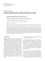
The total distortion in a pair (x, y) after data hiding is
expressed as follows (see Figure 1(a)):
D
DE
=|H − h|=|2 · h + b − h|=|h + b|.
(2)
The distortion of the prediction error expansion (PEE) can
be calculated in the same fashion. Let
m be a predicted pixel
value of a pixel m, then d

= m− m is the prediction error. The
prediction error expansion hides one bit of data as follows
(see Figure 1(b)):
d

= 2 · d + b.
(3)
Hence, the distortion generated by prediction error expan-
sion is
D
PE
=


d

− d


=|
2 · d + b − d|=|d + b|.
(4)
Note that the distortion of the difference errors expansion
and prediction errors expansion are similar in nature.
Rationale for New St rategy. From the above analysis, we can
see that the distortion of both methods directly depends
on the difference value h or prediction error d.Hence,
we need to find a suitable expansion technique, which has
errors less then
|h| or |d|. The main objective of reversible

watermarking is to find a method which can embed more
data with less distortion. Hence, we present a new strategy.
In this st rategy, each pixel is possibly expanded twice by
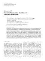
embedding two bits of data. For every pixel, the lower and
upper bounds are computed from eight neighboring pixels.
Let a
i
for i = 1, 2, , 8 be the surrounding pixels for a pixel
a
0
as shown in Figure 2 . The central pixel a
0
and its eight
neighboring pixels define a cell for embedding data. The
neighboring pixels are sorted in ascending order to calculate
the lower and upper bounds as follows:
L
1
=


4
n=1
a
s
n
4

,
L

2
=


8
n
=5
a
s
n
4

,
(5)
where a
s
n
is a set of sorted neighboring pixels. The first
stage of the proposed data hiding technique is represented
as follows:
e
1
= a
0
− L
1
,
(6)
E
1

= 2 · e
1
+ b
1
,(7)
A
1
= L
1
+ E
1
.
(8)
The distortion after the first stage of embedding is given as
D
1
=|A
1
−a
0
|. The second stage of the proposed data hiding
technique is represented as follows:
e
2
= L
2
− A
1
,
(9)

E
2
= 2 · e
2
+ b
2
, (10)
A
2
= L
2
− E
2
.
(11)
The distortion after data hiding is
D
2
=|A
2
− a
0
|
=|
L
1
− L
2
+3· e
1

+2· b
1
− b
2
|.
(12)
Note that the resulted distortion D
2
depends on the utilized
data embedding strategy. In our paper, we use the histogram
shifting strategy for data hiding. Here, (7)and(10)depend
on the differences e
1
and e
2
,respectively.Suchcaseswillbe
explained later in Section 3.1.
In the proposed strategy, we can embed two bits with less
distortion compared to a single embedding. Assume that the
first hidden bit b
1
is 1, second hidden bit b
2
is 1, a = 100,
L
1
= 98, L
2
= 104, and e
1

= 2. First stage of embedding
gives E
1
= 2 · e
1
+ b
1
= 5, the central pixel value A
1
= 103,
and the distance value e
2
= L
2
− A
1
= 104 − 103 = 1. Note
that the distortion D
1
= 3 after first stage of embedding is
the same with distortion of D E and PEE (i.e., e + b). Second
stage of embedding gives E
2
= 2·e
2
+b
2
= 3, the central pixel
A
2

= L
2
−E
2
= 104−3 = 101. The second stage of embedding
reduces distortion from 3 (distortion after the first stage) to
1. The resulted distortion D
2
after hiding two bits of data is
less than the distortion in DE and PEE for a single embedding
(see Figure 1(b)).
In the next section, we present the proposed data hiding
algorithm with all possible scenarios and their distortion.
3. Two-Stage Embedding Algorithm Using
Histogram Shift ing
In the proposed scheme, we can embed data twice with
possibly reduced distortion. As explained in the previous
section, first we calculate L
1
and L
2
using the sorted
neighboring pixels. For data hiding in each stage, we use the
modification of the histogram shifting technique proposed
by Thodi and Rodr
´
ıguez [19]. For the proposed data hiding
technique, we suggest an algorithm to find the appropriate
threshold values T
n

and T
p
(i.e., negative and positive)
similar to the orig inal method. Now, we present the steps
required to encode and decode the hidden data using a two-
stage embedding technique.
Encoding. The algorithm embeds data (b
1
, b
2
) in two stages.
First, the first bit b
1
is hidden using L
1
, and next the second
bit b
2
is hidden using L
2
.
First stage:
E
1
=
⎧
⎪
⎪
⎪
⎪

⎨
⎪
⎪
⎪
⎪
⎩
2 · e
1
+ b
1
,ife
1
∈

T
n
; T
p

,
e
1
+ T
p
+1, ife
1
>T
p
,
e

1
+ T
n
,ife
1
<T
n
,
(13)
where e
1
= a
0
− L
1
.
Note that the expandable set is E
= e ∈ [T
n
; T
p
] and the
shiftable set is S
= e ∈ (−∞; T
n
) ∪ (T
p
; ∞).
The pixel value a
0

after embedding b
1
is changed to
A
1
= L
1
+ E
1
.
(14)
4 EURASIP Journal on Advances in Signal Processing
101 99 103 98
Before
embedding
After
embedding
100
101
102
103
99
98
97
104
100
101
102
103
99

98
97
104
x
x
y
y
L
L
h
X
Y
H
(a)

m

m
98 98
98
98 98
98100
103
Before
embedding
After
embedding
100
101
102

103
99
98
97
104
100
101
102
103
99
98
97
104
m m
d
M
d

(b)
103
100
98 98
102 106
99
97 105
10398 98
102 106
99
97 105
103

10398 98
102 106
99
97 105
101
Before
embedding
After
stage 1
After
stage 2
100
101
102
103
99
98
97
104
100
101
102
103
99
98
97
104
100
101
102

103
99
98
97
104
L
2
L
1
L
2
L
1
L
2
L
1
a aa
e
1
A
1
A
1
A
2
e
2
E
1

E
2
(c)
Figure 1: Different expansion strateg i es ((a) DE; (b) PEE; (c) Two-stage embedding).
a
1
a
2
a
3
a
8
a
0
a
4
a
7
a
6
a
5
Cell
Figure 2: A cell for the proposed scheme.
Second stage: Now, we hide the second bit of data b
2
in A
1
using L
2

. The embedding process is designed as one
E
2
=
⎧
⎪
⎪
⎪
⎪
⎨
⎪
⎪
⎪
⎪
⎩
2 · e
2
+ b
2
,ife
2
∈

T
n
; T
p

,
e

2
+ T
p
+1, ife
2
>T
p
,
e
2
+ T
n
,ife
2
<T
n
,
(15)
where e
2
= L
2
− A
1
.
The pixel value A
1
after embedding b
2
is represented as

follows:
A
2
= L
2
− E
2
.
(16)
T
p
and T
n
are the positive and negative threshold
values. The threshold values can be approximately obtained
using the histogram of the e
1
. Assume that the first and
second stages of embedding have the same payload, and the
histogram’s shape of e
1
and e
2
is similar. Thus, for the given
payload P, the approximate threshold values T
p
and T
n
are
chosen such that

|E| > 0.5 ·|P|,whereE = e
1
∈ [T
n
; T
p
],
and
|E| is the number of elements in the set E. In reality,
due to difference between histogram’s shape of e
1
and e
2
(here, note that the exact value e
2
can be computed only
after hiding data to e
1
), the approximate threshold values
may not be large enough to hide the payload P.Thus,if
that happens, the magnitudes of the threshold values have to
be increased, and the embedding process has to be repeated
30
35
40
45
50
55
60
0

0.2 0.4 0.6 0.8
1
PSNR (dB)
Payload (bpp)
Lena
0; 0
0;
−1
1;
−1
1;
−2
2;
−1
2;
−2
2;
−3
3;
−2
3;
−3
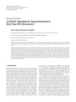
Figure 3: Appropriate threshold values for Lena image.
with new threshold values. Note that the proposed algorithm
can exactly predict the threshold values for the first stage of
embedding. Thus, the approximate threshold values have the
minimal possible magnitudes to hide a necessary payload.
We test the proposed algorithm and find that for most
of payloads the approximate threshold values are suitable
for data h iding. When the payload is large (

≈1 bpp), the
proposed algorithm requires one more iteration. In case
of extreme payloads (
≈1.5 bpp) close to the maximum
possible size (see Figure 7), the proposed algorithm requires
multiple iterations. In Figure 3, we illustrate the appropriate
threshold values for different payloads computed using the
proposed method. If the payload approaches to the point
to be increased (i.e., at 0.18 bpp, 0.29 bpp, or 0.47 bpp),
the proposed method updates the threshold values (see
Figure 3).
Note that, in general, the threshold values for two-stage
embedding have lower magnitude compared to the his-
togram shifting method (see Ta ble 1) due to high embedding
capacity, which results in lower distortion in image. For
example, in case of hiding 120 kbits of data to Lena image,
EURASIP Journal on Advances in Signal Processing 5
the threshold values for histogram shifting are
−2and2,
while for the proposed method they are
−1and1.Such
low threshold values help in improving capacity and low
distortion.
In the decoding process, the lower and upper bounds
calculated using the neighboring pixels remain the same as
in the encoder. Now, we present the steps required to decode
the hidden data.
Decoding. Let (A
2
, a

1
, a
2
, , a
8
) in a single cell be used for
decoding data. The L
1
and L
2
are calculated using the sorted
neighboring pixels as described in (5).
First stage: the decoding process can be described as
e
2
=
⎧
⎪
⎪
⎪
⎪
⎪
⎨
⎪
⎪
⎪
⎪
⎪
⎩


E
2
2

if E
2
∈

2 · T
n
;2· T
p
+1

,
E
2
− T
p
− 1, if E
2
> 2 · T
p
+1,
E
2
− T
n
,ifE
2

< 2 · T
n
,
(17)
where E
2
= L
2
− A
2
.
The second hidden bit b
2
is retrieved using
b
2
= E
2
mod 2, E
2
∈

2 · T
n
;2· T
p
+1

. (18)
After retrieving the data from the pixel value A

2
, the pixel A
1
is computed as foll ows:
A
1
= L
2
− e
2
.
(19)
Second stage: now, we retrieve the first data b
1
from A
1
.
The decoding process is defined as follows:
e
1
=
⎧
⎪
⎪
⎪
⎪
⎪
⎨
⎪
⎪

⎪
⎪
⎪
⎩

E
1
2

if E
1
∈

2 · T
n
;2· T
p
+1

,
E
1
− T
p
− 1, if E
1
> 2 · T
p
+1,
E

1
− T
n
,ifE
1
< 2 · T
n
,
(20)
where E
1
= A
1
− L
1
.
The first hidden bit (b
1
) is retrieved using
b
1
= E
1
mod 2, E
1
∈

2 · T
n
;2· T

p
+1

. (21)
The original pixel value a
0
after retrieving b
1
is recovered as
follows:
a
0
= L
1
+ e
1
.
(22)
The total distortion of the proposed two-stage embedding is
D
2
= A
2
− a
0
,whereA
2
is computed using (16). Here, the
modified pixel A
2

depends on the different scenarios in the
(13)and(15).
Thus, for e
1
∈ [0; T
p
] (expandable, hiding bit b
1
)and
e
2
∈ [T
n
; T
p
] (expandable, hiding bit b
2
), we have
D
2
= L
1
− L
2
+3· e
1
+2· b
1
− b
2

.
(23)
For e
1
>T
p
(shiftable, shifting by T
p
)ande
2
∈ [T
n
; T
p
]
(expandable, hiding bit b
1
), we have
D
2
= L
1
− L
2
+ e
1
+2· T
p
+2− b
1

.
(24)
For e
1
>T
p
(shiftable, shifting by T
p
)ande
2
<T
n
(shiftable,
shifting by T
n
), or e
1
<T
n
(shiftable, shifting by T
n
)ande
2
>
T
p
(shiftable, shifting by T
p
), we have
D

2
= T
p
− T
n
+1.
(25)
For e
1
∈ [T
n
; T
p
] (expandable, hiding bit b
1
)ande
2
>T
p
(shiftable, shifting by T
p
), we have
D
2
= e
1
+ b
1
− T
p

− 1.
(26)
Using the decoding process, we can retrieve the original
pixel value a
0
and the hidden data b
1
and b
2
.Themain
advantage of the proposed method is that the distortion due
to data hiding in the first stage can be reduced in the second
stage efficiently. Hence, we propose the two-stage embedding
scheme to achieve high capacity with low distortion.
3.1. Different Scenarios in Two-Stage Embedding. The min-
imization of distortion due to the first stage at the second
stage depends on e
1
. Based on the value e
1
, there exist three
possible scenarios, namely: removable, half-removable, and
nonremovable cases (see Figure 4).
Removable. In this scenario, the distortion due to the first-
stage embedding is removed completely in the second stage
(i.e., D
2
= 0).
The equality for removing distortion is derived differ-
ently from (23), (24), (25), and (26).

For e
1
∈ [0; T
p
] (expandable, hiding bit b
1
)ande
2
∈
[0; T
p
] (expandable, hiding bit b
2
), we have
e
1
=

L
2
− L
1
− 2 · b
1
+ b
2
3

.
(27)

For e
1
∈ [0; T
p
] (expandable, hiding bit b
1
)ande
2
>T
p
(shiftable, shifting by T
p
), we have
e
1
= T
p
− b
1
+1.
(28)
For e
1
>T
p
(shiftable, shifting by T
p
)ande
2
∈ [0; T

p
]
(expandable, hiding bit b
1
), we have
e
1
= L
2
− L
1
− 2 · T
p
− 2+b
1
.
(29)
For e
1
>T
p
and e
2
>T
p
(both shiftable, shifting by T
p
), the
distortion will be removed completely (i.e., D
2

= 0).
Note that for the e
1
∈ [T
n
;0) or e
2
∈ [T
n
; 0), the
distortion cannot be removed in nature.
Half-Removable. In this scenario, the distortion due to
the first-stage embedding can be removed partially in the
second-stage. The distortion can be reduced or remain the
same. In this case, the modified pixel value A
1
should not
be greater than the upper bound L
2
. Thus, the difference
between the upper bound and modified pixel value A
1
keeps
the sign (i.e., L
2
− A
1
≥ 0). In this case, the second stage
embedding will decrease overall distortion. This scenario will
occur when A

1
≤ L
2
.
6 EURASIP Journal on Advances in Signal Processing
Before
embedding
98 98
102
99
103
103
99
97 100
98 98
102
99
103
103
97 100
98 98
102
99
103
103
97 100
101
99
103
102

101
100
99
98
97
103
102
101
100
99
98
97
103
102
101
100
99
98
97
L
2
L
1
a
L
2
L
1
L
2

L
1
aa
e
1
After stage 1
(hiding “1”)
e
2
E
1
After stage 2
(hiding “1”)
A
1
A
1
A
2
E
2
(a) Removable case
98 98
102
99
103
103
97 100
98 98
102

99
103
103
97 100
98 98
102
99
103
103
97 100
103
100
99 101
102
101
100
99
98
97
103
102
101
100
99
98
97
103
102
101
100

99
98
97
L
2
L
1
a
e
1
Before
embedding
After stage 1
(hiding “1”)
L
2
L
1
a
e
2
E
1
A
1
L
2
L
1
a

A
1
A
2
E
2
After stage 2
(hiding “0”)
(b) Half-removable case
98 98
102
99
103
103
97 100
98 98
102
99
103
103
97 100
98 98
102
99
103
103
97 100
103
102
101

100
99
98
97
96
95
94
103
102
101
100
99
98
97
96
95
94
103
102
101
100
99
98
97
96
95
94
97
L
2

L
1
a
e
1
Before
embedding
L
2
L
1
a
e
2
E
1
A
1
L
2
L
1
a
A
1
A
2
E
2
After stage 1

(hiding “0”)
96
After stage 2
(shifting)
94
(c) Nonremovable case
Figure 4: Different scenarios of the two-stage embedding.
This inequality c an be derived differently in respect of
value e
1
.
For e
1
∈ [0; T
p
], we have
A
1
≤ L
2
,
L
1
+2· e
1
+ b
1
≤ L
2
,

e
1
≤
L
2
− L
1
− b
1
2
.
(30)
For e
1
∈ [0; T
p
]ande
2
∈ [0; T
p
]ore
2
>T
p
, the distortion
D
2
is calculated using (23)or(26), respectively.
For e
1

>T
p
,wehave
A
1
≤ L
2
,
L
1
+ e
1
+ T
p
+1≤ L
2
,
e
1
≤ L
2
− L
1
− T
p
− 1.
(31)
Similarly, for the difference e
2
∈ [0; T

p
], the distortion D
2
is
calculated using (24). Note that for the difference e
2
>T
p
,
the distortion D
2
becomes 0 (i.e., the cell belongs to the
removable case).
Nonremovable. In this scenario, the distortion will increase
after the second stage of embedding. This scenario occurs
when e
1
< 0orA
1
>L
2
.
The inequality A
1
>L
2
can be rewritten similarly with
the half-removable case.
For e
1

∈ [0; T
p
], we have
e
1
>
L
2
− L
1
− b
1
2
.
(32)
In this case, for e
2
∈ [T
n
;0) or e
2
<T
n
, distortion D
2
is
calculated using (23)or(25), respectively.
For e
1
>T

p
,wehave
e
1
>L
2
− L
1
− T
p
− 1.
(33)
Similarly, for the difference e
2
∈ [T
n
;0) or e
2
<T
n
, the
distortion D
2
is calculated using (24)or(25), respectively.
EURASIP Journal on Advances in Signal Processing 7
Note that D
2
is always larger than D
1
for both e

1
< 0and
e
2
< 0.
From the above three scenarios, we can see that the
proposed two-stage embedding strategy either removes,
reduces, or increases the distortion. Similarly, the distortion
in the proposed strategy depends on the selected threshold
values. Since the proposed method can embed data twice, the
selected threshold values for a given capacity is less than the
threshold values for histogram shifting. From Table 1,wecan
see that the threshold values for the proposed method are 25–
50 percent lower. In some cases where the required payload
is low, the threshold values are the same. Note that the
distortion depends on the threshold values as well as the pop-
ulation of pixels (cells) that cause distortion. In the proposed
two-stage embedding method, the cells of the different cases
(i.e., removable, half-removable, and nonremovable) c ause
different distortion impact. The nonremovable cells do not
cause distortion at al l . The distor tion of the half-removable
cells after the double embedding in our method is less than
a sing le embedding in DE or PEE. The nonremovable cells
cause higher distortion than that of DE and PEE under the
same thresholds. Thus, in order to estimate the performance
of the proposed method we h ave to analyze the distortion
impact of the different cells unified to the specific classes
as removable, half-removable, and nonremovable for the
proposed two-stage embedding method, and expandable and
shiftable for the histogram shifting method.

3.2. Efficiency of the Two-Stage Embedding. The efficiency
can be estimated numer ically by computing the portioned
distortion of the different cells for the two-stage embedding
and the histogram shifting. Such an analysis may help
evaluate the distortion impact of the removable, half-
removable, and nonremovable cells to the total distortion.
Since, the PSNR is the logarithmic measure of the MSE
(see (34)), the distortion impact of different pixels (cells) can
be calculated as an impact to the MSE,
PSNR
= 10 · log
10

255
2
MSE

, (34)
where MSE is the mean squared error,
MSE
=
1
m · n
n−1

i=0
m
−1

j=0



I

i, j

−
K

i, j



2
=
1
m · n
SE,
(35)
where n, m are the height and w idth of the image, I is the
original image, K is the modified image, and SE is the total
squared error.
The total squared error (SE) can be calculated as follows:
SE
= SE
0
+SE
1
+SE
2

,
(36)
where
SE
0
= 0ifI

i, j

∈ removable cells,
SE
1
=



I

i, j

− K

i, j



2
if I

i, j


∈ half-removable cells,
SE
2
=



I

i, j

− K

i, j



2
if I

i, j

∈
nonremovable cells.
(37)
From (35)and(36), derive the PSNR as follows:
PSNR
= 10 · log
10


m · n · 255
2
SE
1
+SE
2

. (38)
Thus, the total distortion (PSNR) can be estimated using
the squared errors of all the half-removable cells (SE
1
)and
nonremovable cells (SE
2
).
In our tests, we compare the squared errors (SE) and
population of the half-removable and nonremovable cells
(for the proposed method), and the expandable and shiftable
cells (for the histogram shifting method). To illustrate the
performance better, we study the squared error of the cells
for Lena images versus the threshold values and payloads for
Lena image. The results are reported in Table 1.
When the payload is 70 kbits, the proposed two-stage
embedding method has 21,138 half-removable cells with
squared error 21,102, and 77,151 nonremovable cells with
squared error 266,157. The total squared error is 287,259,
which causes PSNR 47.72 dB. For the same payload, the
histogram shifting method has 70,000 expandable cells with
squared error 71,144, and 166,113 shiftable cells with squared

error 409,255. The total squared error is 487,399, which
causes PSNR 45.25 dB. Thus, when the payload is 70 kbits,
the total squared error of the proposed method is 200,140
lower, and the PSNR is 2.47 dB higher. For larger payloads
such as 120 and 150 kbits, the PSNR value of the proposed
method is 1.31 and 0.83 dB higher, respectively. Hence, the
PSNR value for the proposed method is better than that of
the histogram shifting method.
3.3. Overflow and Underflow Problems. An important issue
in data hiding is to avoid overflow or underflow errors where
the modified pixels exceed the 8-bit range [0; 255]. These
problematic pixels should be skipped from the embedding
process. Such pixels are called skipped cells that can exceed
the boundary (i.e., A
1
< 0, A
1
> 255 or A
2
< 0,
A
2
> 255). Note that the skipped original cells and some
modified cells which can cause overlapping with unmodified
cells should be marked in the location map; otherwise,
decoding will not be possible (refer to [19]). In this method,
the decoder probes the embedding environment through
the simulation. Note that the encoder does not modify
the skipped cells which cause overflow/underflow. Thus,
the simulation of the embedding process in the decoder

has the overflow/underflow in the same cells as in the
encoder. However, the simulation of embedding also causes
overflow/underflow for some cells that were modified during
data hiding. These overlapped cells have to be marked in
8 EURASIP Journal on Advances in Signal Processing
Table 1: Populations of cells from different scenarios and sets versus different capacities for Lena image.
Two-stage embedding
Payload kbits T
n
; T
p
Half-removable case Nonremovable case
Total SE PSNR [dB]
Population SE Population SE
70 −1;0 21,138 21,102 77,151 266,157 287,259 47.72
120
−1;1 64,100 132,453 90,292 743,415 875,869 42.89
150
−1;2 69,290 277,756 111,507 1,500,101 1,777,857 39.82
Histogram shifting [19]
Capacity kbits T
n
; T
p
Expandable set Shiftable set
Total SE PSNR [dB]
Population SE Population SE
70 −1;1 70,000 78,144 166,113 409,255 487,399 45.25
120
−2;2 120,000 277,651 141,098 906,021 1,183,672 41.58

150
−3;3 150,000 580,788 105,744 1,310,011 1,890,799 38.99
3. Recover header and data
- Define LSB
h
from P ={data; LSB
h
}.
- Define data.
-Recoverh using LSB
h
.
Begin
Encoder:
Given:
Image (I)
Data
1. Prepare data and image
- Define space for header (30 pixels)
h
={I(1,1),I(1, 2), I(1,3), , I(1,30)}
- Collect LSB of the h (LSB
h
)
2. Define thresholds (T
n
T
p
)
- Define cells (compute L

1
and e
1
)
-GetT
n
and T
p
, such that
|E| > 0.5P,whereE = e
1
 [T
n
; T
p
]
Decoder:
Given:
Begin
Modified image (I
m
)
1. Read header
- Define thresholds T
n
, T
p
and index i
3. Data hiding
i = i +1

−
|
P|! = 0
3.1 Define i-th cell
- Compute L1, L2, and el.
Update payload II:
P
= {P
3
, P
4
, , P
n
}
,
P
= {P
2
, P
3
, , P
n
}
or skip
3.2 Overflow/underflow test
- Define E.x
E.
a E.b E.c E.d
−−−
+

+++
+
+
Update payload I: P
= {LM; P}
4. Embed header
- Embed header (He)toh by LSB
substitution
Define modified image I
m
End
End
2. Data extraction
i
= i − 1
−
i>30
2.1 Define i-th cell
- Compute L
1
,,L
2
and e
1
.
2.3 Decode data using second
2.3 Decode data using first and
2.2 Overflow/underflow test
- Define A


and A

Read LM
1
= P
1
−
0 ≤ A

≤ 255
0
≤ A

≤ 255
+
LM
1
= 1
−
Read LM
2
= P
2
+
“D.a”
Update payload D
P ={P
2
, P
3

, , P
n
}
P ={P
3
, P
4
, , P
n
}
“D.d ”
−
LM
2
= 0
+
“D.c”
Define original image I
Assign cell’s index i
= 31 (skip first 30 cells)
Assign cell’s index i (from header)
-DefinepayloadP ={data; LSB
h
}
- Define binary header: He = (T
n
, T
p
, i)
2

3.3 Embed b
1
= P
1
using (13), (14)
3.3 Embed b
1
= P
1
, b
2
= P
2
using (13)–(16)
LM = “1”
LM
= “01” LM = “00”
stage only
(20)–(22)
second stages (19)–(22)
“D.b”
Figure 5: Flowchart of the encoder and decoder.
EURASIP Journal on Advances in Signal Processing 9
the location map. Such a solution causes some additional
problems. The decoder can not know the proper data hidden
in the encoder side. Thus, the verification test (see below)
in the encoder and decoder must use the same data. In our
method this data is called “test bits.” Note that hiding “0”
causes distortion less than hiding “1” to the same cell for a
positive difference value. Thus, sometimes hiding “1” causes

overflow/underflow, but hiding “0” does not. In this case,
decoder does not know the proper data and may make wrong
decision about the cell. Such a wrong decision is triggered
by the wrong location map bits, that will cause the cascade
misclassification for the rest of the location map and will
also provide wrong recovered data. We solve this problem
by adjusting the “test bits” as “1” for positive e and “0” for
negative.
Since the proposed method can hide two bits into a
single cell, the problem of overflow/underflow can occur in
any stage of embedding. Hence, we need one or two bits to
identify the overlapping cells. There are four possible cases
regarding the overflow/underflow problems for the encoder.
3.3.1. Overflow/Underflow Test for Encoder
Input. The cell for testing (i.e., (a
0
, a
1
, a
2
, , a
8
)); data to
hide b
1
and b
2
; threshold values T
n
and T

p
.
Output. Case of the cell (i.e., E.a, E.b, E.c, or E.d); location
map bit(s) when the case of cell does not belong to E.d.
Preprocessing. Calculate A
1
and A
2
using (14)and(16). For
0
≤ A
2
≤ 255, process the verification test as follows.
Calculate the test differences d
1
and d
2
:
d
1
= A
2
− L
1
, d
2
= L
2
− A
2

.
(39)
Hide the test bits to the test differences d
1
and d
2
as follows:
D
i
=
⎧
⎪
⎪
⎪
⎪
⎨
⎪
⎪
⎪
⎪
⎩
2 · d
i
+ b
t
if d
i
∈

T

n
; T
p

,
d
i
+ T
p
+1 ifd
i
>T
p
,
d
i
+ T
n
if d
i
<T
n
,
(40)
where i
= 1, 2; D
1
and D
2
are the modified test differences; b

t
is the test bit. If d
1
or d
2
is negative, b
t
is 0; otherwise, b
t
is 1.
Calculate the test pixel values A

and A

:
A

= D
1
+ L
1
, A

= L
2
− D
2
.
(41)
Define the proper case for the tested cell:

(E.a) if a cell has A
1
< 0orA
1
> 255, then we mark the cell
as “1” in the location map. No bit can be embedded
into this cell;
(E.b) if a cell has 0
≤ A
1
≤ 255 and A
2
< 0orA
2
> 255,
then we mark the cell as “01.” In this case, only one bit
can be hidden during the first stage of embedding;
(E.c) if a cell has 0 ≤ A
1
≤ 255, 0 ≤ A
2
≤ 255, and A

< 0,
A

> 255 or A

< 0, A


> 255, then we mark the cell
as “00” in the location map. Here, we use a test bit to
identify whether the cell is to be skipped or not. In
this case, the mark identifies the cell can contain two
bits of hidden data;
(E.d) if the cell does not belong to the skipped set after the
two-stage data hiding process (0
≤ A

≤ 255 and 0 ≤
A

≤ 255), then no marker is used. No marker means
two bits of successful data hiding .
Similar to the encoder, there are three possible situations
regarding the overflow/underflow problems for the decoder.
3.3.2. Overflow/Underflow Test for Decoder
Input. Cell for testing (A
0
, a
1
, a
2
, , a
8
); one or two bits
from the location map, if necessary; threshold values T
n
and
T

p
.
Output. Case of the cell (i.e., D.a, D.b, D.c, or D.d).
Preprocessing. For a tested cell, process as follows: assume
that A
2
= A
0
,whereA
0
is the modified central pixel of the
tested cell. Process the verification test using (39), (40), and
(41). Get test pixel values A

and A

.
Define the proper case for the tested cell:
If a cell has A

< 0, A

> 255 or A

< 0, A

> 255, then
the cell was marked in the location map.
(D.a) If the first location map bit for current cell is “1,” no
bit was embedded into this cell. Otherwise, read the

second bit of the location map and check (D.b)-(D.c).
The cell remains the same as original.
(D.b) If the first and second bits of the location map for
the current cell are “01,” the current cell was modified
during the first stage of embedding. In this c ase, the
cell contains one bit of hidden data.
(D.c) If the first and second bits of the location map for
the current cell are “00,” the current cell was modified
during the first and second stages of embedding. In
this case, the cell contains two bits of hidden data.
(D.d) If a cell has 0
≤ A

≤ 255 and 0 ≤ A

≤ 255,
then the cell was not marked in the location map and
was modified during the first and second stages of
embedding. In this case, the cell contains two bits of
hidden data.
The location map is necessary for recovering data and
should be hidden to image as part of payload. The exper-
imental results show that the location map size is almost
neglig ible when compared to full capacity. Fortunately, the
location map is not necessary sometimes.
4. Algorithms for Encoder and Decoder
The encoder and decoder of the proposed method are
presented in Figure 5 .
Encoder contains four main steps: “Preparation of data
and image (i.e., initialization),” “Definition of threshold val-

ues,” “Data hiding,” and “Embedding header information.”
10 EURASIP Journal on Advances in Signal Processing
30
35
40
45
50
55
60
0 0.1 0.2 0.3 0.4 0.5 0.6 0.7 0.8 0.9 1
PSNR (dB)
Payload (bpp)
Lena
(a)
Barbara
0 0.1 0.2 0.3 0.4 0.5 0.6 0.7 0.8 0.9 1
PSNR (dB)
Payload (bpp)
20
25
30
35
40
45
50
55
60
(b)
Mandrill
30

25
20
35
40
45
50
55
0 0.1 0.2 0.3 0.4 0.5 0.6 0.7 0.8 0.9 1
PSNR (dB)
Payload (bpp)
(c)
Airplane
30
25
35
40
45
50
65
60
55
0 0.1 0.2 0.3 0.4 0.5 0.6 0.7 0.8 0.9 1
PSNR (dB)
Payload (bpp)
(d)
Peppers
Proposed
Lee et. al.
0 0.1 0.2 0.3 0.4 0.5 0.6 0.7 0.8 0.9 1
PSNR (dB)

Payload (bpp)
25
30
35
40
45
50
55
60
Thodi & rodriguez (D3)
Thodi & rodriguez (P3)
(e)
Boat
Proposed
Lee et. al.
25
30
35
40
45
50
55
60
0 0.1 0.2 0.3 0.4 0.5 0.6 0.7 0.8 0.9 1
PSNR (dB)
Payload (bpp)
Thodi & rodriguez (D3)
Thodi & rodriguez (P3)
(f)
Figure 6: Experimental results.

EURASIP Journal on Advances in Signal Processing 11
20
25
30
35
40
45
50
55
60
0 0.2 0.4 0.6 0.8 1 1.2 1.4 1.6 1.8
PSNR (dB)
Payload (bpp)
Airplane
Lena
Peppers
Barbara
Boat
Mandrill
Figure 7: Embedding ability of the proposed method.
Step 1 embeds header information into a certain location,
and copies the original values and embeds into another
location in order to recover the original value. Header
information includes a proper payload. Step 2 defines proper
threshold values. Step 3 embeds data into image. Here, the
block “Update payload I” inserts location map bit (bits) to
the first position of the payload stream (i.e., P
={LM; P}).
The block “Update payload II” removes hidden bit (bits)
from the payload stream. Note that according to the ( 13)–

(16) the proposed method may hide zero, one, or two bits. In
case of hiding zero bits, the block “Update payload II” skips
updating the payload stream. Data hiding process stops when
the last bit from the payload stream P is embedded into the
image (i.e.,
|P|=0). If the number of the available cells is
not enough for hiding payload P, increase thresholds values
and repeat steps 3 and 4.
Decoder contains three main steps: “Read header,” “Data
extraction,” and “Recover header and data.” Step 1 defines
the initial parameters for decoding (threshold values T
n
, T
p
and index i). Cell with index i is the last modified cell in the
encoder. Step 2 recovers the hidden payload and the original
image. The block “Update payload D” removes the location
map bit(bits) from the payload stream P. Step 3 recovers the
original data where header information is embedded.
5. Exp erimental Results
The proposed two-stage reversible data hiding algorithm is
tested over the six well-known uncompressed 512
× 512
grayscale images: Lena, Barbara, Mandrill, Peppers, Boat,
and Airplane. Performances of the proposed algorithm
are compared with well-known methods of Thodi and
Rodr
´
ıguez [14, 19], and Lee et al. [20]. Figure 6 presents
the PSNR values for various payloads in different grayscale

images. From Figure 6, we can see that the PSNR value
of the proposed two-stage embedding is better than that
of the existing methods. Particularly in high payloads, the
proposed scheme shows better performance. The results
clearly indicate the advantage of the two-stage embedding
strategy.
For better understanding, the threshold values and
squared errors used in our experiments and the respective
number of cells in the half-removable and nonremovable sets
for Lena image are reported in Table 1. The population of the
cells and squared error in each set depends on the type of
images and selected threshold values. From Ta ble 1,wecan
see that the population in the nonremovable set increases
with increase in capacity, which makes its performance
worse. Since some of the nonremovable cells can be used for
data hiding in any one of the stages, the overall performance
of the proposed two-stage embedding is better than that of
the well-known methods in the literature.
Figure 7 shows the PSNR values for different payloads.
From Figure 7, we can see that the maximum payload for
Lena, Airplane, Barbara, Peppers, Boat, and Mandrill images
is 1.83, 1.79, 1.48, 1.77, 1.67, and 1.21 bpp, respectively. We
also consider the capacity of the proposed method based on
the given minimum allowable distortion. Hence, we select
the minimum allowable distortion for each image based
on the maximum capacity of the method P3 of Thodi and
Rodr
´
ıguez [14]. In the case of the Air plane image, their
maximum payload is 0.98 bpp and its corresponding PSNR

value is 32.1 dB. If the 32 dB is the minimum allowable
distortion, our method achieves 1.51 bpp, which is 50 percent
more than the capacity of the histogram shifting method.
A similar observation can be made about the Barbara,
Lena, Peppers, Boat, and Mandrill images. In the case of
Mandrill, the maximum capacity is less than the other tested
images due to its irregularity in the image, but our capacity
is still higher than the existing methods. From the result, we
can say that the proposed two-stage embedding algorithm
can have lower distortion under the same capacity compared
to the existing methods.
6. Conclusion
This paper presents a novel two-stage reversible watermark-
ing algorithm with higher capacity and lower distortion. The
proposed strategy can embed data twice using the lower
and upper bounds computed from the sorted neighboring
pixels. The distortion due to embedding data in the first
stage can be removed at rare occurrences, mostly reduced, or
hardly increased in the second stage. In general, data hiding
distorts the original images. Nonremovable case distorts the
image like any other methods including histogram shifting
approach. Even though the population of the removable
case is small, this set never distorts. In case of the half-
removable set, this method distorts less. As a result, this
method distorts image less. Also, the problems of overflow
and underflow are handled using a special location map
similar to the method presented in [19]. Experimental results
clearly indicate the advantage of the proposed method versus
well-known methods in reversible watermarking in terms of
ratio of capacity over distortion.

12 EURASIP Journal on Advances in Signal Processing
Acknowledgments
This work was supported by the Catholic University of
Korea, IT R&D program (Development of anonymity-based
u-knowledge security technology, 2007-S001-01), by the
Ministry of Knowledge Economy, Korea, under the ITRC
supervised by the National IT Industry Promotion Agency
(NIPA-2010-C1090-1001-0004), by the Ministry of Culture,
Sports and Tourism and Korea Culture Content Agency in
the Culture Technology (CT) Research and Development
Program, and by the Ministry of Education, Science and
Technology under the super vision of National Research
Foundation for 3DLife (FP7). Authors thank the reviewers
for their valuable comments which improve the quality of
this paper.
References
[1] F. Mintzer, J. Lotspiech, and N. Morimoto, “Safeguarding
digital library contents and users: digital watermarking,” D-
Lib Magazine, vol. 3, no. 12, pp. 33–45, 1997.
[2] J. Fridrich, M. Goljan, and R. Du, “Lossless data embedding
for all image formats,” in Security and Watermarking of
Multimedia Contents IV, vol. 4675 of Proceedings of SPIE,pp.
572–583, January 2002.
[3] M. van der Veen, F. Bruekers, A. Leest, and S. Cavin,
“High capacity reversible watermarking for audio,” in Security,
Steganography, and Watermarking of Multimedia Contents VI,
vol. 5020 of Proceedings of SPIE, p. 111, January 2003.
[4] A. Van Leest, M. van der Veen, and F. Bruekers, “Reversible
watermarking for images,” in Security, Steganography, and
Watermaking of Multimedia Contents VI, vol. 5306 of Proceed-

ings of SPIE, pp. 374–385, January 2004.
[5] M. U. Celik, G. Sharma, A. M. Tekalp, and E. Saber,
“Reversible data hiding,” IEEE International Conference on
Image Processing, vol. 2, pp. II/157–II/160, 2002.
[6] B. Yang, M. Schmucker, W. Funk, C. Busch, and S. Sun,
“Integer DCT-based reversible watermarking for images
using companding technique,” in Securit y, Steganography,
and Watermaking of Multimedia Contents VI, vol. 5306 of
Proceedings of SPIE, pp. 405–415, January 2004.
[7] B. Yang, M. Schmucker, C. Busch, X. Niu, and S. Sun,
“Approaching optimal value expansion for reversible water-
marking,” in Proceedings of the 7th Multimedia and Security
Workshop, pp. 95–101, August 2005.
[8]G.Xuan,J.Chen,J.Zhu,Y.Q.Shi,Z.Ni,andW.Su,
“Lossless data hiding based on integer wavelet transform,”
in Proceedings of the IEEE Workshop on Multimedia Signal
Processing, pp. 312–315, St. Thomas, Virgin Island, December
2002.
[9] G. Xuan, Y. Q. Shi, Z. C. Ni et al., “High capacity lossless data
hiding based on integer wavelet transform,” in Proceedings of
the IEEE International Symposium on Circuits and Systems, vol.
2, pp. II29–II32, 2004.
[10]G.Xuan,C.Yang,Y.Zhen,Y.Q.Shi,andZ.Ni,“Reversible
data hiding based on wavelet spread spectrum,” in Proceedings
of the IEEE 6th Workshop on Multimedia Sig nal Processing,pp.
211–214, Siena, Italy, 2004.
[11] D. Zou, Y. Q. Shi, Z. Ni, and W. Su, “A semi-fragile
lossless digital watermarking scheme based on integer wavelet
transform,” IEEE Transactions on Circuits and Systems for Video
Technology, vol. 16, no. 10, pp. 1294–1300, 2006.

[12] L. Kamstra and H. J. A. M. Heijmans, “Reversible data
embedding into images using wavelet techniques and sorting,”
IEEE Transactions on Image Processing, vol. 14, no. 12, pp.
2082–2090, 2005.
[13] H. J. Kim, V. Sachnev, Y. Q. Shi, J. Nam, and H. G. Choo,
“A novel difference expansion transform for reversible data
embedding,” IEEE Transactions on Information Forensics and
Securit y, vol. 3, no. 3, pp. 456–465, 2008.
[14] D . M. Thodi and J. J. Rodr
´
ıguez, “Expansion embedding
techniques for reversible watermarking,” IEEE Transactions on
Image Processing, vol. 16, no. 3, pp. 721–730, 2007.
[15] J. Tian, “Reversible data embedding using a difference expan-
sion,” IEEE Transactions on Circuits and Systems for Video
Technology, vol. 13, no. 8, pp. 890–896, 2003.
[16] W. Hong, T. S. Chen, and C. W. Shiu, “Reversible data
hiding based on histogram shifting of prediction errors,” in
Proceedings of the 2nd International Symposium on Intelligent
Information Technology Application Workshop (IITA ’08),pp.
292–295, December 2008.
[17] H. C. Huang, I. H. Wang, and Y. Y. Lu, “High capacity
reversible data hiding with adjacent-pixel-based difference
expansion,” in Proceedings of the 4th International Conference
on Innovative Computing, Information and Control (ICICIC
’09), pp. 639–642, December 2009.
[18] Z. Ni, Y. Q. Shi, N. Ansari, W. Su, Q. Sun, and X. Lin,
“Robust lossless image data hiding,” in Proceedings of the IEEE
International Conference on Multimedia and Expo (ICME ’04),
vol. 3, pp. 2199–2202, Taipei, Taiwan, 2004.

[19] D . M. Thodi and J. J. Rodr
´
ıguez, “Reversible watermarking
by prediction-error expansion,” in Proceedings of the 6th IEEE
Southwest Symposium on Image Analysis and Interpretation,
vol. 6, pp. 21–25, Lake Tahoe, Calif, USA, March 2004.
[20] S. Lee, C. D. Yoo, and T. Kalker, “Reversible image water-
marking based on integer-to-integer wavelet transform,” IEEE
Transactions on Information Forensics and Security, vol. 2, no.
3, pp. 321–330, 2007.
[21] V. Sachnev, H. J. Kim, J. Nam, S. Suresh, and Y. Q. Shi,
“Reversible watermarking algorithm using sorting and pre-
diction,” IEEE Transactions on Circuits and Systems for Video
Technology, vol. 19, no. 7, pp. 989–999, 2009.
[22] A. M. Alattar, “Reversible watermark using difference expan-
sion of triplets,” in Proceedings of the International Conference
on Image Processing (ICIP ’03), pp. 501–504, September 2003.
[23] A. M. Alattar, “Reversible watermark using difference expan-
sion of quads,” in Proceedings of the IEEE International
Conference on Acoustics, Speech, and Signal Processing,pp.
III377–III380, May 2004.
[24] A. M. Alattar, “Reversible watermark using the difference
expansion of a generalized integer transform,” IEEE Transac-
tions on Image Processing, vol. 13, no. 8, pp. 1147–1156, 2004.