Báo cáo hóa học: " Research Article Markov Modelling of Fingerprinting Systems for Collision Analysis" pptx
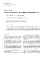
Bạn đang xem bản rút gọn của tài liệu. Xem và tải ngay bản đầy đủ của tài liệu tại đây (707.07 KB, 10 trang )
Hindawi Publishing Corporation
EURASIP Journal on Information Security
Volume 2008, Article ID 195238, 10 pages
doi:10.1155/2008/195238
Research Article
Markov Modelling of Fingerprinting Systems for
Collision Analysis
Neil J. Hurley, F
´
elix Balado, and Gu
´
enol
´
e C. M. Silvestre
School of Computer Science and Informatics, University College Dublin, Belfield, Dublin 4, Ireland
Correspondence should be addressed to Neil J. Hurley,
Received 8 May 2007; Revised 19 October 2007; Accepted 3 December 2007
Recommended by S. Voloshynovskiy
Multimedia fingerprinting, also known as robust or perceptual hashing, aims at representing multimedia signals through compact
and perceptually significant descriptors (hash values). In this paper, we examine the probability of collision of a certain general class
of robust hashing systems that, in its binary alphabet version, encompasses a number of existing robust audio hashing algorithms.
Our analysis relies on modelling the fingerprint (hash) symbols by means of Markov chains, which is generally realistic due to the
hash synchronization properties usually required in multimedia identification. We provide theoretical expressions of performance,
and show that the use of M-ary alphabets is advantageous with respect to binary alphabets. We show how these general expressions
explain the performance of Philips fingerprinting, whose probability of collision had only been previously estimated through
heuristics.
Copyright © 2008 Neil J. Hurley et al. This is an open access article distributed under the Creative Commons Attribution License,
which permits unrestricted use, distribution, and reproduction in any medium, provided the original work is properly cited.
1. INTRODUCTION
Multimedia fingerprinting, also known as robust or per-
ceptual hashing, aims at representing multimedia signals
through compact and perceptually significant descriptors
(hash values). Such descriptors are obtained through a hash-
ing function that maps signals surjectively onto a sufficiently
lower-dimensional space. This function is akin to a cryp-
tographic hashing function in the sense that, in order to
perform nearly unique identification from the hash values,
perceptually different signals—according to some relevant
distance—must lead with high probability to clearly differ-
ent descriptors. Equivalently, the probability of collision (P
c
)
between the descriptors corresponding to perceptually dif-
ferentsignalsmustbekeptlow.Differently than in cryp-
tographic hashing, signals that are perceptually close must
lead to similar robust hashes. Despite this difference with re-
spect to cryptographic hashing, the probability of collision
remains the parameter that determines the “resolution” of a
method for identification purposes.
A large number of robust hashing algorithms have been
proposed recently. This flurry of activity calls for a more sys-
tematic examination of robust hashing strategies and their
performance properties. In this paper, we take a step in that
direction by examining the probability of collision of a cer-
tain general class of robust hashing systems, rather than an-
alyzing a particular method. In its binary alphabet version,
the class considered broadly encompasses several existing al-
gorithms, in particular, a number of robust audio hashing
algorithms [1–4]. We will show that the M-ary alphabet ver-
sion of the class provides an advantage over the binary ver-
sion for fixed storage size. In order to keep our exposition
simple, other issues such as robustness to distortions or to
desynchronization are not considered in this analysis. The
study of the tradeoffs brought about by the simultaneous
consideration of these issues is left as further work. We must
also note that we will be dealing with unintentional collisions
due to the inherent properties of the signals to be hashed.
A related problem not tackled in this paper is the analysis
of intentional forgeries of signals—perhaps under distortion
constraints—in order to maximize the probability of colli-
sion.
The class of fingerprinting systems that we will study
in this paper can be considered as consisting of two in-
dependent blocks. Denoting the multimedia signal to be
hashed by a continuous-valued N-dimensional vector x
=
(x[1], ,x[N]), in the first feature extraction block,afunc-
tion, f (
·), is applied to extract a set of L feature vectors,
2 EURASIP Journal on Information Security
which we assume to be real-valued with dimension K.The
feature extraction function is
f (
·):R
N
−→ R
K
×···×
L−1
R
K
,(1)
so that f (x)
= (D
1
, , D
L
)withD
m
= (D
m
[1], , D
m
[K])
for m
= 1, , L.
The second block can be termed as the hashing block,in
which the continuous feature vector values are mapped to a
finite alphabet of hash symbols, that is, quantized. In many
methods, this hashing block is implemented through the ap-
plication of a scalar hashing function to each scalar feature
vectorvalue,whichwedenoteas
h(
·):R −→ H ,(2)
where H is the alphabet of hash symbols whose size is given
by M
|H |.
In any hashing system, a distance measure must be estab-
lished in order to determine the closeness between hash val-
ues. The commonly used distance for comparing sequences
formed by discrete-alphabet symbols is the Hamming dis-
tance. This distance is defined as the number of times that
symbols with the same index differ in the two sequences.
Therefore, when comparing any two M-ary symbols their
Hamming distance can only take the values 0 or 1.
As already stated, our aim is to investigate the proba-
bility of collision—also termed in some works false positive
probability—of the general type of system described above,
under certain assumptions that we will give next. Given a dis-
tance measurement, the probability of collision is simply the
probability that the fingerprints (hashes) of two independent
signals are closer than some preestablished threshold accord-
ing to the distance measurement established. Our analysis
will rely on the fact that the feature vector values are gen-
erally highly correlated, due to the synchronization require-
ments of a fingerprinting system. This high degree of cor-
relation frees the observer of a segment of x (or a distorted
version of it) from the need to know its exact alignment with
the complete original signal used to store the fingerprint dur-
ing the acquisition process (in which the reference hash is
obtained for subsequent comparisons). For example, in the
Philips method [5] the features are extracted by processing x
frame-by-frame on a set of heavily overlapped frames, which
creates the conditions for our analysis. In the following, we
will consider the case in which dependencies within a feature
vector can be modelled as a continous-valued, discrete-time
Markov chain. In particular, we assume that
Pr
D
m
[i] | D
m
[1], , D
m
[i −1]
= Pr
D
m
[i] | D
m
[i −1]
(3)
for all m
= 1, , L. Furthermore, we assume that the pro-
cess is stationary, that is, with statistics independent of i.We
will also focus without loss of generality on one particular
element m of the feature vector. Hence, we will write the rel-
evant random variables of the feature vector as D and D
to
represent the distributions of the feature value at i and i
−1,
respectively, for any i, dropping the implicit index m.
We characterize next the Markov chain of the hash sym-
bols. Define F h(D)tobethediscretehashsymbolgener-
ated by application of the hashing function to a particular
element of the feature vector. We will assume that the se-
quence F[i] forms a discrete-valued, discrete-time Markov
chain, with transition probabilities defined by
π
s,r
Pr
F = k
s
| F
= k
r
(4)
for all the M
2
pairs (k
s
, k
r
) ∈ H
2
.
Finally note that, although methods which deal with real-
valued fingerprints could be deemed in principle to belong to
this class (using very large values of M), they rely on the use
of mean square error distances instead of the Hamming dis-
tance. Thus, their study is not covered by the class of methods
studied here.
Notation
Lowercaseboldfaceletterssuchasx represent column vec-
tors, while matrices are represented by upper case Roman let-
ters such as X. diag(x) is a matrix with the elements of x in
the diagonal and zero elsewhere. The symbols I and O denote
the identity and the all-zero matrices, respectively, whereas 1
denotes an all-ones vector, all of suitable size depending on
the context. tr(X) denotes the trace of X. The vec(
·)opera-
tor stacks sequentially the columns of an n
× m matrix into
an nm
× 1columnvector.Thesymbol⊗ denotes the Kro-
necker (or direct) product of two matrices, and
denotes
their Hadamard (component-wise) product. Finally, δ
ij
de-
notes the Kronecker delta function.
2. PROBABILITY OF COLLISION
We firstly define s as the amount of bits required to store a
single M-ary hash symbol, that is,
s log
2
M. (5)
To fix a point of operation, we consider hash sequences of n/s
symbols (assumed integer) which have fixed bit size n (stor-
age size). We investigate the probability of collision between
two such independent sequences of symbols generated from
the Markov chain with M
×M transition matrix Π
π
s,r
,
whoseelementsaredefinedin(4). Note that Π is a column-
stochastic matrix, so that 1
T
Π = 1
T
.
The probability of collision is simply the probability that
two such hash sequences are closer than a given threshold
under the distance measure established. Write d
n
to repre-
sent the Hamming distance between the sequences. Let γn/s
be the Hamming distance below which we consider two se-
quences of storage size n bits to be identical, with 0
≤ γ<1
and assuming γn/s integer for simplicity. Using this thresh-
old, the probability of collision between two sequences of
storage size n is
P
c
= Pr
d
n
≤ γn/s
. (6)
Neil J. Hurley et al. 3
In order to approximate this probability, observe that for any
two n/s-length sequences of symbols their overall Hamming
distance is
d
n
=
n/s
i=1
d[i](7)
with d[i] the Hamming distance between the ith elements
of the two sequences. If the random variables d[i] were in-
dependent, we could apply the central limit theorem (CLT)
to d
n
for large n, in order to compute the probability (6).
Although there are short-term dependencies created by the
Markov chain, these vanish in the long term. Then we may
invoke a broader version of the CLT for locally correlated sig-
nals [6]. In summary, the result in [6] states that, provided
the second and third moments of
|d[i]| are bounded, then
d[i] tends to the normal distribution. Finally, notice that
d
n
is discrete, and then applying the CLT entails approximat-
ing a distribution with support in the positive integers using
a distribution with support in the whole real line.
Assuming that the distribution of d
n
may be approxi-
mated by a Gaussian for large n, we only need its mean E
{d
n
}
and variance V{d
n
} to characterize it. The probability of col-
lision can then be approximated as
P
c
≈ Q
E{d
n
}−γn/s
V{d
n
}
(8)
with Q(x) (1/
√
2π)
∞
x
exp (−ξ
2
/2)dξ. We tackle the com-
putation of the statistics required for this approximation in
Section 3, and particular cases in Section 5.
Alternatively, the exact computation of (6)involvesenu-
merating all cases generating a Hamming distance lower than
or equal to γn/s, that is,
P
c
=
γn/s
k=0
Pr {d
n
= k}. (9)
We investigate this direct approach in Section 4. Finally, in
Section 6 we propose a Chernoff bound to P
c
, which is useful
when the CLT assumption is not accurate or when the exact
computation presents computational difficulties.
3. MEAN AND VARIANCE OF HAMMING DISTANCE
In this section, we derive the mean and variance of the Ham-
ming distance using the Markov chain of symbol transitions
Π,definedby(4). To proceed, we assume that Π represents
an irreducible, aperiodic Markov chain.
We denote as v
i
∈ H
2
the pair of simultaneous values
of two independent hash sequences at time i. The Hamming
distance between the elements of v
i
is denoted by d(v
i
)such
that d(
·):H
2
→{0, 1}. Also, for convenience we denote the
nonnegative integer associated with the concatenation of the
bit representation of the two components of v
i
by c(v
i
). For
instance, with M
= 4, a possible value of v
i
is (1,3); in this
particular case, d(v
i
) = 1andc(v
i
) = 7, as the bit representa-
tion of the components is 01 and 11, respectively. We define
next the M
2
× 1vectorμ
i
with components Pr {v
i
= h},for
all possible M
2
values of h ∈ H
2
sorted in natural order,
that is, according to c(h). The pairs thus defined constitute a
new Markov chain with column-stochastic transition matrix
B Π
⊗Π,with⊗ the Kronecker product. Therefore,
μ
i
= Bμ
i−1
= B
i−1
μ
1
, (10)
for all indices i>1. Denote the equilibrium distribution of
this Markov chain as μ; then
Bμ
= μ,B
i
−→ μ1
T
as i −→ ∞. (11)
If B is symmetric, then the symbols are equally likely in equi-
librium and μ
= 1/M
2
1.
Some more definitions will be required in order to for-
malize the derivation of the probabilities associated with a
given Hamming distance sequence. Firstly, we define two in-
dicator vectors i
0
and i
1
,bothofsizeM
2
× 1. The elements
of the vector i
k
are defined to be all zeros except for those
elements at positions in μ such that Pr
{v = (v
1
, v
2
)} corre-
sponds to a pair with Hamming distance d(v
1
, v
2
) = k,which
are set to 1. It is easy to see that i
0
= vec(I) and i
1
= vec(11
T
−
I). Now, defining β
i
(Pr {d[i] = 0},Pr{d[i] = 1})
T
,we
can write the distribution of elemental Hamming distances
at the index i as
β
T
i
=
i
T
0
μ
i
, i
T
1
μ
i
. (12)
Observe next that the element at the position (n, m)of
the matrix B
j−i
diag(μ
i
), with j>i, gives the joint probability
Pr
{v
j
= c
−1
(n −1),v
i
= c
−1
(m −1)} with c
−1
(·) the unique
inverse of c(
·). Using this matrix, we can write the joint prob-
ability of a pair of elemental distances as
Pr
d[j] = k, d[i] = l
= i
T
k
B
j−i
diag(μ
i
)i
l
(13)
with j>i.
Using the probabilities (12)and(13), we can derive the
mean and variance of the Hamming distance between two
independent hash sequences of n/s symbols, assuming that
the process starts in the equilibrium distribution (11). This is
tantamount to assuming μ
1
= μ, in which case μ
i
= μ and
β
i
= β [i
0
, i
1
]
T
μ, that is, we can drop the index i and write
Pr
{d[i] = k}=Pr {d = k}. When the initial symbol is cho-
sen with uniform probability from H this condition holds if
the transition matrix is symmetric. Even if all values for the
initial symbol are not equiprobable in reality, the assumption
is not too demanding whenever convergence to equilibrium
is fast. We investigate a more general case for binary hashes
in Section 5.
Noting that (7) is a sum of dependent variables, we have
E
d
n
=
n/s
i=1
E
d[i]
,
(14)
V
d
n
=
n/s
i=1
E
d
2
[i]
+2
j>i
E
d[i]d[j]
−E
2
d
n
.
(15)
4 EURASIP Journal on Information Security
Notice that, as d
2
[i] = d[i] because the Hamming distance
only takes values in
{0, 1}, the first summand in (15)isjust
(14). We compute next the different summands required to
obtain E
{d
n
} and V{d
n
}. Denote the equilibrium mean and
variance of d[i]asE
{d} and V{d},respectively.Theafore-
mentioned mean and second moment are given by
E
{d}=Pr {d = 1}=i
T
1
μ,
(16)
wherewehaveused(12) and the equilibrium assumption.
Hence (14)isgivenby
E
{d
n
}=
n
s
E
{d}.
(17)
Next, consider the sum of the elemental distance covari-
ances. If the elemental distances were independent, we would
have
E
j>i
d[i]d[j]
=
j>i
E
d[i]
E
d[j]
=
n(n −s)
2s
2
E
2
{d}.
(18)
Taking into account the dependencies, we have instead,
E
j>i
d[i]d[j]
=
j>i
Pr
d[i] = 1, d[j] = 1
.
(19)
Using next (12), (13), and the equilibrium assumption we
can compute (19)as
E
j>i
d[i]d[j]
=
i
T
1
j>i
B
j−i
diag(μ)i
1
.
(20)
In Appendix A, we develop this expression to show that the
variance (10) of the Hamming distance between two n/s-
length hash sequences is
V
{d
n
}=
n
s
V
{d}+2i
T
1
G diag(μ)i
1
(21)
with G given by (A.9).
4. THE STOCHASTIC PROCESS OF
ELEMENTAL DISTANCES
In this section, we will investigate the stochastic process of
elemental distances, that is, the process that generates the
sequence
{d[1],d[2], , d[n]}. Through an analysis of this
process, we arrive at a full expression for the probability of
collision, which is exact in the case of binary hashing se-
quences with symmetric transition matrices. This is possible
because, as we will show, the elemental distance process is it-
self a Markov chain when s
= 1 and the transition matrix is
symmetric. Even for the case s>1, we note that the elemen-
tal distance process is well approximated by a Markov chain,
and then the expression obtained for the probability of colli-
sion can be interpreted as a good approximation to the true
collision probability.
To understand the process of elemental distances,
{d[1],d[2], , d[n]}, we consider the conditional probabil-
ity of d[i +1]givend[i]. Define the matrix A with compo-
nents a
kl
Pr {d[i +1]= k − 1 | d[i] = l − 1}.From(12)
and (13) we have that
a
kl
=
i
T
k
−1
B diag(μ
i
)i
l−1
Pr
d[i] = l −1
=
i
T
k
−1
(Π ⊗Π)diag(μ
i
)i
l−1
i
T
l
−1
μ
i
.
(22)
Define Ψ
i
as the matrix such that μ
i
= vec Ψ
i
. Using i
o
=
vec(I), note that diag(μ
i
)i
0
= vec(Ψ
i
I), where is the
Hadamard product. Now using the identity (vec P)
T
(Π ⊗
Π)(vec Q) = tr QΠ
T
P
T
Π for any matrices P and Q of ap-
propriate size [7], we have that
a
11
=
tr[(Ψ
i
I)Π
T
Π]
tr[Ψ
i
I]
.
(23)
Equation (23) represents a weighted sum of the diagonal el-
ements of Π
T
Π, with the weights depending on μ
i
and sum-
ming to 1. Similarly, using i
1
= vec(11
T
−I) and diag (μ
i
)i
1
=
vec(Ψ
i
−Ψ
i
I), we have
a
12
=
tr[(Ψ
i
−Ψ
i
I)Π
T
Π]
tr[Ψ
i
−Ψ
i
I]
.
(24)
Note that (24) is a weighted sum of the off-diagonal elements
of Π
T
Π with weights depending on μ
i
and summing to one.
The remaining two components of A are given by a
21
= 1 −
a
11
and a
22
= 1 −a
21
.
It follows that, whenever the diagonal elements of Π
T
Π
are all equal and the off-diagonals are all equal, the depen-
dence of A on μ
i
factors from (23)and(24), and A is inde-
pendent of the time-step i. In this case, the process of elemen-
tal distances is itself a stationary Markov chain. Let us assume
that Π has the structure Π
= aI+bSwithS 11
T
− Iand
a+(M
−1)b = 1. In this case, as S
2
= (M −2)S+(M −1)I, we
can see that Π
T
Π = Π
2
= a
I+b
Switha
a
2
+ b
2
(M −1)
and b
2ab + b
2
(M − 2). As we have discussed above, this
is the structure that allows to cancel the dependence on μ
i
in (23)and(24). For M = 2, observe that symmetry implies
that Π is always of the form above, and then the conditions
are always fullfilled in that case.
On the other hand, even when the elemental distances
do not follow a Markov chain, since μ
i
→ μ, the equilib-
rium probability, the elemental distance process is well ap-
proximated by the Markov chain with transition matrix A
obtained by replacing Ψ
i
in (23)and(24)withΨ, such that
vec Ψ
= μ. From now on, we will refer loosely to the elemen-
tal distance Markov chain, meaning, when appropriate, the
Markov chain derived from this approximation.
Neil J. Hurley et al. 5
4.1. Probability of collision
Using (23)and(24), define p a
11
, the probability of a tran-
sition from 0
→ 0, and q 1 −a
12
, the probability of a tran-
sition 1
→ 1, in the elemental distance Markov chain. Let
β
1
= (β
10
, β
11
)
T
be the initial distribution of the elemental
distance. Consider a sequence, d
= (d[1], , d[n])
T
,such
that d
n
=
n
i
=1
d[i] = k. Then there are k positions in d
at which d[i]
= 1. Presume for the moment that d[1] = 1.
Starting with a block of ones, d consists of blocks of ones,
interweaved with blocks of zeros. Let n
0
be the number of
blocks of zeros and n
1
be the number of blocks of ones. Con-
sider the case n
1
= r ≥ 1. Then either n
0
= r,inwhich
case, the sequence ends with a block of zeros, or n
0
= r − 1
in which case the sequence ends with a block of ones. Given
that there are in total k ones in the sequence, it is possible to
count the number of different types of transitions that occur
in the sequence and hence the probability that this sequence
can occur. Indeed, if D represents the random variable mod-
elling an n-bit Hamming distance sequence, then
Pr
D=d | d[1]=1
=
⎧
⎪
⎪
⎪
⎪
⎪
⎪
⎪
⎨
⎪
⎪
⎪
⎪
⎪
⎪
⎪
⎩
q
k−r
p
n−k−r
(1−q)
r
(1−p)
r−1
,
n
1
= n
0
= r,
q
k−r
p
n−k−r+1
(1−q)
r−1
(1−p)
r−1
,
n
1
= r, n
0
= r − 1.
(25)
For l
= 0andl = 1, define P
l
(r) Pr {d
n
= k, n
1
= r |
d[1] = l}.ToevaluateP
1
(r), we enumerate all the different
ways that a sequence d with d
n
= k and n
1
= r can occur.
This amounts to counting the number of ways that k ones
can be subdivided into r blocks and n
− k zeros can be sub-
divided into r or r
− 1 blocks. With the blocks constructed,
interweaving the blocks creates the sequence d.Indeed,from
the total of k
−1 possible positions at which the sequence of
ones can be split, it is necessary to choose r
− 1 positions.
Hence there are
k−1
r
−1
different ways to select r blocks of
ones, and similarly
n−k−1
r
−1
to select r blocks of zeros, and
n−k−1
r
−2
to select r −1 blocks of zeros. Thus,
P
1
(r) =
k −1
r
−1
n −k − 1
r
−1
×
q
k−r
p
n−k−r
(1 −q)
r
(1 − p)
r−1
+
k −1
r
−1
n −k − 1
r
−2
×
q
k−r
p
n−k−r+1
(1 −q)
r−1
(1 − p)
r−1
.
(26)
Now,
Pr
{d
n
= k}=
k
r=1
β
11
P
1
(r)+β
10
P
0
(r). (27)
Assuming k<n
−k; p, q>0, using an analogous argument to
derive P
0
(r) and gathering terms, we arrive at the expression
Pr {d
n
= k}=p
n−k−1
q
k
k
−1
r=0
k −1
r
φ
r+1
q
φ
r
p
×
n −k − 1
r +1
β
10
φ
p
+
n −k − 1
r
β
11
+ p
n−k
q
k−1
k
−1
r=0
n −k − 1
r
φ
r
q
φ
r+1
p
×
k −1
r
β
10
+
k −1
r +1
β
11
φ
q
,
(28)
where φ
p
(1 − p)/pand φ
q
(1 −q)/q.
Expression (28) gives the exact probability of collision
when the sequence of elemental distances is a Markov chain.
In other cases, it will lead to an approximation. Conse-
quently, the analysis is exact for s
= 1andΠ symmetric, in
which case p (
= q) can be determined easily from A = Π
2
.
5. BINARY HASHES WITH SYMMETRIC
TRANSITION MATRIX
In this section, we derive expressions for the particular case
s
= 1withΠ symmetric. In this case, some simplifications
on the general expressions derived above are possible. Define
firstly the 2
×2matrices
H
11
1
2
11
T
,H
12
I −H
11
. (29)
Note that the first matrix is idempotent, that is, H
2
11
= H
11
,
and then so is the second, H
2
12
= H
12
; a further consequence
of the definitions is H
11
H
12
= H
12
H
11
= O. Assuming sym-
metry, then for some
−1 ≤ θ<1, we can write the binary
transition matrix as
Π
= H
11
+ θH
12
. (30)
With θ so defined, it can be checked that as n
→∞,(17)
and (21)reduceto
E
d
n
=
n
2
,
V
d
n
=
n
4
1+θ
2
1 −θ
2
−
θ
2
2(1 −θ
2
)
2
.
(31)
While (31) holds under the assumption that the distribution
of β
1
is the equilibrium distribution, it is also possible to de-
rive the exact mean and variance of d
n
from an arbitrary ini-
tial distribution. This case is interesting, since, although the
symbol sequences are assumed to be generated from inde-
pendent sources, at the application level, the first bit of the
hash sequence corresponding to the input signal is some-
times aligned with that of the hash sequences in the database.
We can handle this scenario by assuming that the distance
between the initial pair of bits is zero.
6 EURASIP Journal on Information Security
Before proceeding, note that the transition matrix for the
elemental distance process is A
= Π
2
and, from (30), we can
write
A
= H
11
+ θ
2
H
12
.
(32)
5.1. Exact mean and variance
With β
1
= (β
10
, β
11
)
T
, as before, the initial distribution of
the elemental distances, it is convenient to define the vectors
h
1
(1/2)(1, 1)
T
and h
2
(1/2)(1, −1)
T
and write β
1
=
h
1
+ ψh
2
with
ψ β
10
−β
11
. (33)
Note that H
1i
h
j
= δ
ij
h
j
and h
T
i
h
i
= 1/2. Following the same
argument as previously, and defining e
1
h
1
− h
2
,weob-
tain analogous expressions to (16)and(20) for this case as
follows:
E
d
n
=
n
i=1
e
T
1
P
2i−2
β
1
,
(34)
j>i
E
d[i],d[ j]
=
j>i
e
T
1
Π
2(j−i)
diag
Π
2i−2
β
1
e
1
.
(35)
The summands in (34) are sums of terms of the form
h
T
u
H
1v
h
w
, which are nonzero only when u = v = w.Fur-
thermore, since the coefficient of H
12
in Π is θ, it follows that
the coefficient of H
12
in Π
2i−2
is θ
2i−2
. Hence, summing the
geometric series,
E
{d
n
}=
n
i=1
h
T
1
H
11
h
1
−ψθ
2i−2
h
T
2
H
12
h
2
=
n
2
−
α
2
ψ,
(36)
where
α
1
−θ
2n
1 −θ
2
. (37)
On the other hand, the summands in (35)aresumsofterms
of the form h
T
p
H
1q
diag(H
1u
h
v
)h
w
, which are nonzero only
when u
= v and p = q, in which case they take the value
h
T
p
diag (h
u
)h
w
.Now,observethatdiag(h
1
)h
w
= h
w
/2and
diag (h
2
)h
w
= h
3−w
/2. Hence, (35)reducestoasumover
four terms, T
1
, T
2
, T
3
,andT
4
,where
T
1
= h
T
1
H
11
diag
H
11
h
1
h
1
=
1
4
,
T
2
=−h
T
1
H
11
diag
θ
2(i−1)
ψH
12
h
2
h
2
=−
1
4
θ
2(i−1)
ψ,
T
3
= h
T
2
θ
2(j−i)
H
12
diag
H
11
h
1
h
2
=
1
4
θ
2(j−i)
,
T
4
=−h
T
2
θ
2(j−i)
H
12
diag
θ
2(i−1)
ψH
12
h
2
h
1
=−
1
4
θ
2(j−1)
ψ.
(38)
In Appendix B, we use (38) to show that the variance of a
symmetric binary hash is
V
{d
n
}=
n
4
1+θ
2
1 −θ
2
−
αθ
2
2(1 −θ
2
)
−
α
2
ψ
2
4
. (39)
Noting that α
→ (1 −θ
2
)
−1
as n →∞, this expression coin-
cides with (31)asn
→∞when ψ = 0.
6. CHERNOFF BOUNDING
For large n and small probabilities the CLT can exhibit large
deviations from the true probabilities. This is due to the fact
that the CLT gives an approximation based only on the two
first moments of the real distribution. Also, the exact com-
putation (28) can run into numerical difficulties due to the
combinatorials involved. Then, it is interesting to see what
can be obtained by means of Chernoff bounding on (6).
Apart from the interest of a strict upper bound, this strat-
egy also provides the error exponent followed by the integral
of the tail of the distribution of d
n
.
The Chernoff bound on the probability of collision is
given by
P
c
≤ min
ξ>0
E
exp
−ξ
d
n
−γn
=
min
ξ>0
exp (ξγn)·E
exp
−ξd
n
.
(40)
The expectation in (40) cannot be expanded as a product
of elemental expectations due to the implicit dependencies.
However, using the transition matrix A of the elemental dis-
tance Markov chain and defining σ (1exp (
−ξ))
T
,wecan
efficiently compute it as
E
{exp (−ξd
n
)}=σ
T
(A diag(σ))
(n/s)−1
β
1
. (41)
It is not possible to optimize this expression analytically in
closed-form. Nonetheless, numerical optimization can be
easily undertaken, as (41)isjustaweightedsumofpowers
of exp (
−ξ).
7. EMPIRICAL RESULTS
Matlab source code and data assoicated with the empiri-
cal results given below can be downloaded from http://www
.ihl.ucd.ie.
7.1. Synthetic Markov chains
To test the validity of the expressions presented and the ac-
curacy of the CLT approximation, random binary and 4-ary
hash sequences were drawn from the Markov chain model.
For the binary case, the transition matrix Π in (30) is used
with θ
= 0.8. The generator matrix used for the 4-ary hashes
used Π
4
Π ⊗ Π (note: no relationship with B here). The
initial hash symbols were drawn from the equilibrium (uni-
form) distribution. This corresponds to 4-ary sequences gen-
erated by concatenation of binary pairs. The collision proba-
bility was measured empirically, using 1.9
× 10
6
trials in the
binary case and 4.9
×10
7
trials in the 4-ary case. In Figure 1,
these empirical probabilities are plotted against the CLT ap-
proximation, using the mean and variance given by (17)and
(21), respectively. Also shown is the theoretical expression,
calculated as
γn/s
k=0
Pr {d
n
= k} using (28) and the elemen-
tal distance Markov chain. This demonstrates the accuracy
Neil J. Hurley et al. 7
350300250200150100500
n
CLT approximation
Theoretical
Empirical
Chernoff bound
10
−12
10
−10
10
−8
10
−6
10
−4
10
−2
10
0
P
c
2-ary
4-ary
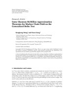
Figure 1: Probability of collision for independent hash sequences
generated from the Markov chain with transition matrices Π given
by (30) with θ
= 0.8 (binary case) and Π ⊗Π (4-ary case), plotted
against the storage size n. Collisions are determined by the threshold
γn/s in expression (6) with γ
= 0.3.
of the elemental distance Markov chain approximation for
4-ary hashes.
The CLT approximation has good agreement in the bi-
nary case for n>20, but is significantly less accurate for 4-
ary hashes. This is due to the fact that in the second case, the
pdf of d
n
is significantly skewed as zero distances are more
likely to happen. Due to this, the CLT approximation un-
derstimates the tail of the true distribution. The Chernoff
bound, also shown in Figure 1, follows the same shape as the
exact distribution and is tighter for high values of n than the
CLT approximation.
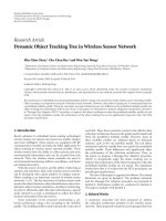
7.2. The Philips method
We show in this subsection how the Markov modelling that
we have described is applicable to the hashing method pro-
posed by Haitsma et al. [1], commonly known as the Philips
method. Moreover we show how previous work on mod-
elling this particular method allows to obtain analytically the
parameters of the Markov chain.
In previous work [8], we developed a model that allows
the analysis of the performance of the Philips method un-
der additive noise and desynchronisation. Using this model,
the transition matrix of the Markov chain associated to the
bitstream of the Philips hash can be determined analytically
as follows. In [8] we analysed the bit error that results from
desynchronization, the lack of alignment between the orig-
inal framing used in the acquisition stage and the framing
that takes place in the identification stage.
In particular, we showed that for a given band (i.e., a par-
ticular feature value D
m
in this paper) the probability of error
350300250200150100500
n
Empirical
Theoretical
10
−3
10
−2
10
−1
10
0
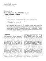
P
c
Figure 2: The empirical probability of collision of the Philips
method is plotted against storage size n and compared with the the-
oretical expression (28). The theoretical plot uses a binary transi-
tion matrix with p
Δ
(m) calculated using (42) and the correlation
coefficient ρ
Δ
(m) determined empirically from hash sequence data.
Hashes are generated from normally distributed i.i.d input signals.
Each frame corresponds to 0.37 seconds of a 44.1 kHz signal.
for a desynchronization of k indices in x is well approximated
by
p
k
(m)
1
π
arccos
ρ
k
(m)
, (42)
where ρ
k
is the correlation coefficient corresponding to that
band and that level of desynchronization. This model was
shown therein to give very good agreement with empirical
results, even with real audio (and hence nonstationary) in-
put signals.
This same formula can be applied to determine the tran-
sition probabilities 0
→ 1or1→ 0 of the hash bits within
a given signal. To this end we only need to observe that two
overlapped frames which generate consecutive hash bits are
in fact desynchronized by the number of indices where there
is no overlap. Denoting this value by Δ and using k
= Δ
in (42), it follows that the binary Markov chain model of
Section 5 with θ
= 2p
Δ
− 1 can be used to determine the
probability of collision for this method. Figure 2 shows the
accuracy of this model against empirical results, for a range
of hash sequence lengths from n
= 20 to n = 320, with
the Philips method applied to the hashing of normally dis-
tributed i.i.d input signals.
It is relevant to compare our Markov chain analysis with
the collision probability for the Philips method previously
examined in [5],inwhichitisreferredtoasthe“probability
of false alarm.” Therein, it was assumed that d[i]weremutu-
ally independent, leading straightforwardly to E
{d
n
}=n/2
and V
{d
n
}=n/4. With the CLT approximation, from (8),
8 EURASIP Journal on Information Security
this yields the following expression for the collision proba-
bility,
P
c
≈ Q
(1 −2γ)
√
n
, (43)
which is independent of the transition probability. To obtain
agreement with empirical data, in [5] this expression is mod-
ified to account for dependencies using a heuristic correction
factor 1/3, that is,
P
c
≈ Q
1
3
(1
−2γ)
√
n
. (44)
Considering our own CLT approximation (8), we observe
that, letting n
→∞in (36)and(39), the correction factor
with respect to the independent case actually tends to
1+θ
2
1 −θ
2
. (45)
In the results presented in Figure 2, θ
=−0.83 and hence
the correction factor for this value of θ is 1/2.33
≈ 0.43. In
summary, our analysis is able to tackle dependencies without
resorting to any heuristics.
7.2.1. Real audio signals
We examine the validity of our analysis for real audio sig-
nals, by carrying out a collision analysis on hashes gener-
ated using the Philips method on three real audio signals al-
ready used in [1, 8]: “O Fortuna” by Carl Orff,“Saywhatyou
want” by Texas, and “Whole lotta Rosie” by AC/DC (16 bits,
44.1 kHz). Using the parameters of the original algorithm
describedin[1], a 32-bit block, corresponding to N
b
= 32
frequency bands, is extracted from each frame. Each frame
corresponds to 0.37 seconds of audio and the degree of over-
lap between frames is 1/32. Hence, from each audio file, a
hash block of N
f
×32 bits is extracted, where the number of
frames N
f
is between 20000 and 30000. Our collision analysis
is applied by estimating a single empirical correlation coeffi-
cient
ρ from the entire hash block. We then use our model to
predict the probability of collision between hash sequences
drawn from the first 200 000 elements of the entire sequence
of N
f
×32 bits. The results are shown in Figure 3.
Although our model assumes stationarity, which is
clearly not the case for real audio signals, good agreement
is found between the model predictions and empirical data.
The greatest discrepancy appears in the AC/DC audio and
may be due to greater dynamics in this song. To improve the
results, we could apply the approach used in [8], where real
audio signals are approximated by stationary stretches and
apply our model separately to each stretch. While this ap-
proach can provide the probability of collision within each
stationary stretch, combining these into an overall probabil-
ity of collision could prove problematic.
8. CONCLUSION
We have examined the probability of collision of a certain
general class of robust hashing systems that can be described
350300250200150100500
n
Te x a s
Orff
AC/DC
10
−3
10
−2
10
−1
10
0
P
c
Figure 3: The empirical probability of collision of the Philips
method for three real audio signals is plotted against storage size n
and compared with the theoretical expression (28). Dots stand for
empirical values whereas lines stand for theoretical results.
by means of Markov chains. We have given theoretical ex-
pressions for the performance of general chains of M-ary
hashes, by deriving the mean and variance of the distance
between independent hashes and applying a CLT approxi-
mation for the probability distribution. We have been able to
derive an expression for the distribution, which is exact for
binary symmetric hashes and gives a very good approxima-
tion otherwise. We have confirmed the accuracy of the Gaus-
sian distribution on binary hashes once the hash sequence is
sufficiently large. Moreover, we derived the binary transition
matrix for the Philips method and showed that the Markov
chain model has very good agreement with empirical results
for this method. While we have shown that for M>2, M-ary
chains have an advantage over binary chains from the point
of view of collision, higher order alphabets will inevitably
lead to a degradation of performance under additive noise
and desynchronisation error. The performance tradeoffs that
result will be examined in future work.
APPENDICES
A. VARIANCE OF AN M-ARY HASH SEQUENCE
In this appendix, we detail the computation of (20)inorder
to obtain V
{d
n
}. Firstly, see that the following identity that
holds:
j>i
B
j−i
=
n/s−1
i=1
n
s
−i
B
i
=
n
s
n/s−1
i=1
B
i
−
n/s−1
i=1
iB
i
. (A.1)
Neil J. Hurley et al. 9
Define T
n/s−1
i
=1
iB
i
and S
n/s−1
i
=1
B
i
. Then
T(I
−B)
2
= B
n/s
n
s
(B
−I) −B
+B. (A.2)
Since 1 is an eigenvector of B, (I
−B) is not invertible. Instead,
notice that
Tμ
=
n/s−1
i=1
iμ =
n(n −s)
2s
2
μ (A.3)
which implies
TW
=
n(n −s)
2s
2
W(A.4)
with W μ1
T
. Similarly,
S(I
−B) = B −B
n/s
,SW=
n −s
s
W(A.5)
and therefore,
S(I
−B)
2
= B −B
2
+B
n/s+1
−B
n/s
. (A.6)
Using (A.2), (A.4), (A.5), and (A.6), we get
n
s
S
−T
(I −B)
2
+W
=
n −s
s
B −
n
s
B
2
+B
n/s+1
+
n(n
−s)
2s
2
W.
(A.7)
Observe that, since WB
= μ(1
T
W) = μ1
T
= W,
W
I −B)
2
+W
=
W, (A.8)
which implies that ((I
−B)
2
+W)
−1
is a right identity of W.
Hence, using the definition
G B
n −s
s
I
−
n
s
B+B
n/s
(I −B)
2
+W
−1
(A.9)
(A.7)canberewrittenas
n
s
S
−T
=
n(n −s)
2s
2
W+G. (A.10)
Note also that
i
T
1
·W diag(μ)·i
1
= (i
T
1
μ)
2
= E
2
{d}.
(A.11)
Using (A.10)and(A.11), the sum of the covariances (20)is
found to be
j>i
E
d[i]d[j]
=
n(n −s)
2s
2
E
2
{d}+ i
T
1
G diag(μ)i
1
.
(A.12)
As n
→∞,
G
−→ B
n −s
s
I
−
n
s
B
(I −B)
2
+W
−1
+W. (A.13)
Using (17)and(A.12)in(15)wefinallyobtain(21).
B. VARIANCE OF BINARY SYMMETRIC
HASH SEQUENCE
In this appendix, we compute the sum of covariances (35),
necessary to obtain the variance of a symmetric binary hash
using (15). We will use (38) for this computation. We note
firstly the following identities:
j>i
θ
2(j−i)
=
n−1
i=1
(n −i)θ
2i
,
j>i
θ
2(j−1)
=
n−1
i=1
iθ
2i
,
j>i
θ
2(i−1)
=
n−1
1=1
(n −i)θ
2i−2
,
n−1
i=1
iθ
2i
=
θ
2
−θ
2n
θ
2
+ n(1 −θ
2
)
(1 −θ
2
)
2
.
(B.1)
Using the definition in (37), we can write
n−1
i=1
iθ
2i
=
θ
2
(1 −θ
2
)
α
−
nθ
2n
(1 −θ
2
)
=
θ
2
(1 −θ
2
)
α + nα
−
n
(1 −θ
2
)
.
(B.2)
Therefore,
j>i
E
d[i]d[j]
=
j>i
1
4
1+θ
2(j−i)
−
ψ
4
θ
2(i−1)
+ θ
2(j−1)
=
n(n −1)
8
+
n
4
n−1
i=1
θ
2i
−
1
4
n−1
i=1
iθ
2i
−
ψ
4
n
θ
2
n
−1
i=1
θ
2i
−
1
θ
2
n
−1
i=1
iθ
2i
+
n−1
i=1
iθ
2i
.
(B.3)
Using (37), (B.1), and (37), (B.3)becomes
j>i
E
d[i]d[j]
=
n(n −1)
8
+
n
4
(α
−1) −
1
4
n−1
i=1
iθ
2i
−
ψ
4
n
θ
2
(α −1) −
1 −θ
2
θ
2
n
−1
i=1
iθ
2i
.
(B.4)
Inserting (B.2) into the expression above, we get
j>i
E
d[i]d[j]
=
n(n −1)
8
−
n
4
−
θ
2
α
4(1 −θ
2
)
+
n
4(1 −θ
2
)
−
ψ
4
n
θ
2
α −
n
θ
2
−nα
1
−θ
2
θ
2
−α +
n
θ
2
=
n(n −1)
8
+
θ
2
(n −α)
4(1 −θ
2
)
−
ψ
4
(n
−1)α.
(B.5)
Finally, inserting (36)and(B.5) into (15), we arrive at
(39).
10 EURASIP Journal on Information Security
REFERENCES
[1] J. Haitsma, T. Kalker, and J. Oostveen, “Robust audio hashing
for content identification,” in Proceedings of the International
Workshop on Content-Based Multimedia Indexing (CBMI ’01),
pp. 117–125, Brescia, Italy, September 2001.
[2] M. K. Mihc¸ak and R. Venkatesan, “A perceptual audio hashing
algorithm: a tool for robust audio identification and informa-
tion hiding,” in Proceedings of the 4th International Workshop
on Information Hiding (IHW ’01), vol. 2137 of Lecture Notes
In Computer Science, pp. 51–65, Springer, Pittsburgh, Pa, USA,
April 2001.
[3] S. Baluja and M. Covell, “Content fingerprinting using
wavelets,” in Proceedings of the 3rd European Conference on Vi-
sual Media Production (CVMP ’06), pp. 209–212, London, UK,
November 2006.
[4] S. Kim and C. D. Yoo, “Boosted binary audio fingerprint based
on spectral subband moments,” in Proceedings of the 32nd IEEE
International Conference on Acoustics, Speech, and Signal Pro-
cessing (ICASSP ’07), vol. 1, pp. 241–244, Honolulu, Hawaii,
USA, April 2007.
[5] J. Haitsma and T. Kalker, “A highly robust audio fingerprint-
ing system,” in Proceedings of the 3rd International Conference
on Music Information Retrieval (ISMIR ’02), pp. 107–115, Paris,
France, October 2002.
[6] M. Blum, “On the central limit theorem for correlated random
variables,” Proceedings of the IEEE, vol. 52, no. 3, pp. 308–309,
1964.
[7]J.R.MagnusandH.Neudecker,Matrix Differential Calculus
with Applications in Statistics and Econometrics, John Wiley &
Sons, New York, NY, USA, 2nd edition, 1999.
[8] F. Balado, N. J. Hurley, E. P. McCarthy, and G. C. M. Silvestre,
“Performance analysis of robust audio hashing,” IEEE Trans-
actions on Information Forensics and Security,vol.2,no.2,pp.
254–266, 2007.