Báo cáo hóa học: " Research Article Modified Spatial Channel Model for MIMO Wireless Systems" ppt

Hindawi Publishing Corporation
EURASIP Journal on Wireless Communications and Networking
Volume 2007, Article ID 68512, 7 pages
doi:10.1155/2007/68512
Research Article
Modified Spatial Channel Model for MIMO Wireless Systems
Lorenzo Mucchi,
1
Claudia Staderini,
1
Juha Ylitalo,
2
and Pekka Ky
¨
osti
3
1
CNIT, University of Florence, via santa marta 3, 50139 Florence, Italy
2
Centre for Wireless Communications, University of Oulu, 90014 Oulu, Finland
3
Elektrobit, 90570 Oulu, Finland
Received 13 June 2007; Revised 19 September 2007; Accepted 11 November 2007
Recommended by G. K. Karagiannidis
The third generation partnership Project’s (3GPP) spatial channel model (SCM) is a stochastic channel model for MIMO systems.
Due to fixed subpath power levels and angular directions, the SCM model does not show the degree of variation which is encoun-
tered in real channels. In this paper, we propose a modified SCM model which has random subpath powers and directions and
still produces Laplace shape angular power spectrum. Simulation results on outage MIMO capacity with basic and modified SCM
models show that the modified SCM model gives constantly smaller capacity values. Accordingly, it seems that the basic SCM gives
too small correlation between MIMO antennas. Moreover, the variance in capacity values is larger using the proposed SCM model.
Simulation results were supported by the outage capacity results from a measurement campaign conducted in the city centre of

Oulu, Finland.
Copyright © 2007 Lorenzo Mucchi et al. This is an open access article distributed under the Creative Commons Attribution
License, which permits unrestricted use, distribution, and reproduction in any medium, provided the original work is properly
cited.
1. INTRODUCTION
Future wireless communication aims at higher data rates.
Since the radio spectrum is limited, the requirement of high
spectrum efficiency can be fulfilled by exploiting the spatial
dimension of the radio channel [1]. In sufficiently rich multi-
path environments, the channel capacity can be significantly
increased by using multiple antennas at both the transmitter
and the receiver sides of the link. Multiple-input multiple-
output (MIMO) technique brings a relevant increase not
only in capacity but also in coverage, reliability, and spec-
tral efficiency. In MIMO case, the overall transmit channel
is described as a matrix instead of a vector, and the spatial
correlation properties of the channel matrix define the num-
ber of available parallel channels for data transmission [2, 3].
Depending on the channel gains of the parallel channels,
the MIMO channel can have much higher channel capacity
compared to a single-input single-output (SISO) channel in
the same frequency range and with the same total transmit
power.
The performance of such a system is largely determined
by the MIMO channel characteristics, so it is critical to create
channel models that accurately reflect realistic behavior.
In this paper, the spatial channel model proposed by the
Third Generation Partnership Project (3GPP) [4, 5]isinves-
tigated and compared to a modified SCM model, which was
derived in this study. Comparison is based on simulated and

measured outage capacity. This study was motivated by the
fact that the basic SCM model has fixed signal path directions
and powers within a resolvable delay tap which is expected to
over-simplify the MIMO channel model and thus affect the
simulation results. Since it is important that a MIMO chan-
nel model is a realistic representation of real radio channels
we compared the simulated results also to results obtained
from measured MIMO radio channels. Measurements cam-
paign was carried out in an urban environment.
The rest of the paper is organized as follow: the system
model is described in Section 2, spatial channel modeling is
presented in Section 3, simulation and measurement results
are given in Sections 4 and 5, respectively, and finally, con-
clusions are summarized in Section 6.
2. SYSTEM MODEL
Consider a spatial multiplexing MIMO system with N
T
transmit antennas and N
R
receive antennas. At each time in-
stant n, the system model can be expressed as
y(n)
= H(n)x(n)+η(n),
(1)
2 EURASIP Journal on Wireless Communications and Networking
Table 1: Table of measurements settings.
Propsound property Setting
Center frequency 253 GHz
Transmit power +23 dBm
Chip rate 100 Mchips/s

Code length 511 chips
Number of TX antenna elements 11
Number of RX antenna elements 32
Number of channels 352
Mobile speed 20 km/h
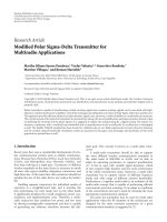
Tx
Path
Sub-path 20
AS
Sub-path 2
Sub-path 1
Sub-path 19
α
.
.
.
.
.
.
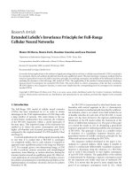
Figure 1: Angular spread model for a nominal path.
where H(n) is the N
R
× N
T
Rayleigh flat fading channel ma-
trix given by
H
=
⎡
⎢

⎢
⎢
⎢
⎣
h
1,1
h
1,2
h
1,N
T
h
2,1
h
2,2
h
2,N
T
.
.
.
.
.
.
.
.
.
.
.
.

h
N
R
,1
h
N
R
,2
h
N
R
,N
T
⎤
⎥
⎥
⎥
⎥
⎦
,(2)
where h
i,j
defines the channel gain from transmit antenna i
and receive antenna j;symbols
x(n)
=

x
1
(n), , x

N
T
(n)

T
(3)
([
∗
]
T
stands for transpose), taken from a modulation con-
stellation A
= [a
1
, , a
N
], are transmitted from each an-
tenna; η(n)isN
R
×1zeromeancomplexcircularlysymmetric
Gaussian noise.
Defining with N
T
the number of the elements at the
transmit array and with N
R
the number of the elements at
the receive array, the instantaneous capacity (in bps/Hz) un-
der a transmit power constraint and assumption that there is
perfect channel state information (CSI) at RX, while there is

no channel state information at the TX, is given by
C
= log

det

I
N
R
+
γ
N
T

HH
H


,
(4)
where I
N
R
is the identity N
R
× N
R
matrix, γ is the signal to
noise ratio at the receiver, H is the channel matrix, and H
H

is
the Hermitian (conjugate transpose) of H.
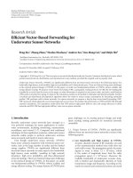
Laplacian PAS
Even number of sub-paths
−θ
4
−θ
3
−θ
2
−θ
1
θ
1
θ
2
θ
3
θ
4
Figure 2: Subpaths distribution with equal power.
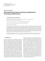
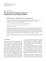
Figure 3: Transmitting antenna array.
In practice, the cumulative distribution function (CDF)
of outage capacity is often used [6]; it is defined as the thresh-
old below which the system capacity will be with a given out-
age probability P
out
:
P
out


C
th

= Pr

C ≤ C
th

,
(5)
where C
th
is the threshold capacity and C is the capacity.
It is evident that the smaller is the spatial correlation be-
tween antennas the larger is the MIMO capacity. The spatial
correlation is dictated by the angular spread of the propa-
gation paths at the transmitter and the receiver. Root mean
square (RMS) angular spread (AS) is given by
φ
RMS
=





K
k=1


φ
k

2
P
A

φ
k


K
k=1
P
A

φ
k

−

φ
M

2
,
(6)
where φ
k
is the kth azimuth AoA and P

A
(φ) is the power az-
imuth spectrum (PAS) and φ
M
is the mean azimuth given by
[7]
φ
M
=

K
k
=1

φ
k

P
A

φ
k


K
k=1
P
A

φ

k

. (7)
The power azimuth spectra at TX and RX are related to the
spatial correlation matrices of the MIMO radio channel at
the TX and RX, respectively. Accordingly, the PAS can be cal-
culated using the Fourier beamforming [8]:
P
A
(φ) = a(φ)
H
Ra(φ),
(8)
where R denotes the corresponding spatial correlation ma-
trices, φ scans the angular aperture, and a(φ) represents the
Lorenzo Mucchi et al. 3
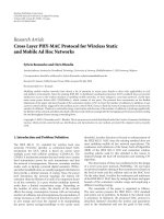
Figure 4: Receiving antenna array.
normalized steering vector of either the TX array or the RX
array and is expressed as
a(φ)
=

1, e
−j2πdsin(φ)/λ
, e
−j4πdsin(φ)/λ
, , e
−jπ(L−1)dsin(φ)/λ

T

,
(9)
where λ is the wavelength, d
= λ/2andT denotes the trans-
pose. Equation (9) is valid only for uniform linear array. The
spatial correlation matrix at the RX side is given by
R
RX
=
⎡
⎢
⎢
⎢
⎢
⎣
ρ
1,1
ρ
1,2
ρ
1,N
R
ρ
2,1
ρ
2,2
ρ
2,N
R
.

.
.
.
.
.
.
.
.
.
.
.
ρ
N
R
,1
ρ
N
R
,2
ρ
N
R
,N
R
⎤
⎥
⎥
⎥
⎥
⎦

, (10)
where ρ
RX
i
1
,i
2
is the complex correlation coefficient at the RX
between antennas i
1
and i
2
given by
ρ
i
1
,i
2
=
E

h
i
1
,j
h
i
∗
2
,j



E



h
i
1
,j


2


h
i
2
,j


2

.
(11)
It is worth to note that the PAS can be calculated by us-
ing (8) which involves a relation between PAS and the spatial
correlation matrix R, while in the 3GPP SCM model the PAS
is given and not calculated. Moreover, the procedure of esti-
mating RMS AS, PAS, and R, shown above for RX side (AoA),

is analogous for TX side (and AoD).
3. SPATIAL CHANNEL MODELLING
The 3GPP SCM model is serving as the basis for evalua-
tion of MIMO performance of candidate MIMO concepts for
UMTS [4]. In the following we first introduce the 3GPP SCM
model and then propose a modification of it.
3.1. 3GPP SCM
The 3GPP spatial channel model has been defined for CDMA
systems with 5 MHz bandwidth and 2 GHz center frequency.
The procedure for obtaining the channel coefficients matrix
isdescribedin[4]. Each of the N received paths has M sub-
paths (cluster). In 3GPP SCM model, each resolvable path
0
0.02
0.04
0.06
0.08
0.1
0.12
0.14
0.16
0.18
Power (linear)
−15 −10 −50 5 1015
AoD azimuth angle (deg)
Modified SCM
SCM
Figure 5: Laplacian PAS with 5 degrees RMS AS with basic and
modified SCM.
0

0.1
0.2
0.3
0.4
0.5
0.6
0.7
0.8
0.9
1
Probability (C<abscissa)
0 5 10 15 20 25 30 35
Channel capacity (bits/s/Hz)
SCM basic 10 dB
SCM basic 20 dB
SCM basic 30 dB
SCM modified 10 dB
SCM modified 20 dB
SCM modified 30 dB
Figure 6: Simulated outage capacity; RMS = 8degrees
is characterized by its own spatial channel parameters: an-
gular spread (AS), angle of departure (AoD), angle of ar-
rival (AoA), and power azimuth spectrum (PAS). The ar-
ray topology at the BS is, for example, a typical 3-sector an-
tenna patterns. The half-power beam width is 70 degrees and
the antenna gain is 14 dB. The receiving antenna element
radiation pattern is, for example, omnidirectional with an-
tenna gain equal to
−1 dB. The resolvable paths amplitudes
are modeled as Rayleigh distributed variables. This implies

a correlation between consecutive elements of the array that
can be modeled with the well-known Jakes model [9]. Sev-
eral measurements show that in an urban environment, the
AS could be relatively narrow, thus implying a higher cor-
relation between the array elements. In order to take into
4 EURASIP Journal on Wireless Communications and Networking
0
0.1
0.2
0.3
0.4
0.5
0.6
0.7
0.8
0.9
1
Probability (C<abscissa)
0 5 10 15 20 25 30 35
Channel capacity (bits/s/Hz)
SCM modified 10 dB
SCM modified 20 dB
SCM modified 30 dB
SCM basic 10 dB
SCM basic 20 dB
SCM basic 30 dB
Figure 7: Simulated outage capacity; RMS = 15 degrees
account this effect, the 3GPP associates 20 subpaths to each
path (Figure 1) to model the AS through their AoA and AoD
at the mobile station and the base station, respectively. The

subpaths are symmetrically placed about the nominal path
direction. It is important to emphasize that the 20 angular
values of the subpaths offsets are fixed (see [4]) and that all
the subpaths have identical powers equal to P/20, where P is
the power associated to the main path. The resulting power
azimuth spectrum (PAS) follows the shape of Laplacian dis-
tribution (Figure 2) with a certain variance, which varies ac-
cording to the chosen environment: urban macrocell, urban
microcell, suburban macrocell. It is expected that due to fixed
subpath directions and powers, the model does not bring all
the variability which is present in real radio channels. More-
over, equally strong subpaths may require large angular sep-
aration in order to obtain eligible AS. This reduces the corre-
lation between MIMO antennas and thus over-estimates the
MIMO capacity.
3.2. Modified SCM model
As discussed above, the 3GPP SCM may not reproduce the
dynamic nature of a real MIMO channel due to its static
modeling of the subpaths. In order to achieve a better match
with the measured channels from the capacity point of view,
a slightly different modeling of the spatial properties is pro-
posed in this paper. We propose to choose the 20 azimuth
angle values of the subpaths at the BS randomly from a uni-
form angular distribution in the interval (
−15, +15) degrees
around the received path delay position and to assign the rel-
ative power values from a Laplace function:
P(φ)
=
1

√
2σ
exp

−
√
2|φ|
σ

,
(12)
where σ is the standard deviation of the Laplacian distri-
bution and φ are the azimuth values chosen according to
0
0.1
0.2
0.3
0.4
0.5
0.6
0.7
0.8
0.9
1
Probability (C<abscissa)
0 5 10 15 20 25 30 35 40 45
Channel capacity (bits/s/Hz)
SCM modified 10 dB
SCM modified 20 dB
SCM modified 30 dB

SCM basic 10 dB
SCM basic 20 dB
SCM basic 30 dB
Figure 8: Simulated outage capacity; RMS = 24 degrees
0
0.1
0.2
0.3
0.4
0.5
0.6
0.7
0.8
0.9
1
Probability (C<abscissa)
0 5 10 15 20 25 30 35 40 45
Channel capacity (bits/s/Hz)
SCM modified 10 dB
SCM modified 20 dB
SCM modified 30 dB
SCM basic 10 dB
SCM basic 20 dB
SCM basic 30 dB
Figure 9: Simulated outage capacity; RMS = 40 degrees.
the uniform distribution. The resultant PAS distribution is
Laplacian. At the MS, the 20 azimuth values of the subpaths
were randomly chosen from uniform distribution, and the
relative power values were assigned according to a uniform
distribution. As a result, the PAS distribution is uniform.

Figure 5 compares the generation of Laplacian PAS, both
in 3GPP SCM method with fixed subpath angles and in the
modified SCM method with random subpath angles. In the
modified SCM case, one possible realization of angles and
powers is depicted. In the basic SCM, angles and powers al-
ways remain unchanged and the specific angular positions of
the subpaths define Laplacian PAS.
Lorenzo Mucchi et al. 5
Configuration A
(a)
Configuration B
(b)
Configuration C
(c)
Configuration D
(d)
Figure 10: Chosen combinations of RX antenna elements. Four antenna elements can be chosen out of 16 dual-polarized (±45 degrees)
antenna elements.
4. SIMULATION RESULTS
Simulations of outage capacity were run using both the 3GPP
SCM model and the modified SCM for a 4
×4 MIMO case. In
each case of comparison, the RMS angular spreads of the ba-
sic and modified SCM models were set to be equal. Thus, at
least two channel parameters are the same, namely, the angu-
lar spread and the delay spread properties (flat fading case).
At the BS, four different RMS AS values were considered: 8,
15, 24, and 40, while at the MS, the RMS AS was set to 35.
An urban macrocell environment was supposed with the mo-
bile station having a speed equal to 20 km/h and the antenna

spacing equal to 0.5 λ for both the BS and the MS.
One simulation run includes 10 000 links, which cor-
responds to 10 000 independent MIMO channel samples
(drops in 3GPP terminology). The results for SNR values of
10 dB, 20 dB, and 30 dB, and for RMS AS value varied be-
tween8and40degreesaredrawninFigures6–9.Thecom-
parison between the 3GPP SCM and the modified SCM case
shows that the modified SCM gives systematically smaller
outage capacity values. The difference is becoming more sig-
nificant as the angular spread is increasing. This obviously
demonstrates the fact that the 3GPP SCM model has a static
nature to bring relatively small spatial correlation values be-
tween MIMO antennas. Furthermore, it does not cover the
extreme channel states in which the propagation paths (sub-
paths) are heavily concentrated in the nominal path direc-
tion.
5. MEASUREMENTS RESULTS
The measurement campaign was held in the city of Oulu,
Finland, in July 2005. Propsound radio channel sounder (the
block diagram and all the details can be found in [10])
has been used in the field measurements. The sounder has
been designed so that it suits very well to realistic radio
channel measurements both in time and spatial domains.
This sounder is based on time division multiplexed (TDM)
switching of transmit and receive antennas. Thus, sequential
radio channel measurements between all possible transmit
(TX) and receive (RX) antenna pairs is achieved.
The setup consists of a BS RX antenna equipped with a
16-element dual polarized planar array (Figure 3)andanMS
TX antenna with an L-shaped 11-element array composed

of two uniform linear arrays (ULA) of vertically polarized
monopoles (Figure 4).
The results shown in this paper are related to the urban
macrocell case: the base station RX antenna height was 32 m
and it was few meters above the average rooftop level. The
mobile station was car-mounted and moved at street level
with a speed of 20 km/h, and the mobile TX antenna height
was 2 m.
The sounding signal consists of chip sequences of typ-
ical spread spectrum signals, maximum length sequences
(M-sequences); measurements were carried out with a code
length of 511, a chip rate of 100 Mchip/s, and a carrier
frequency of 2.53 GHz (Tab le 1 ). The transmit power was
26 dBm.
Since the measured MIMO channel matrices include the
path loss, a proper normalization is required; the normaliza-
tion factor is given by
F
=

1
N
T
N
R
N
T

i=1
N

R

j=1


h
i,j


2

−1
,
(13)
6 EURASIP Journal on Wireless Communications and Networking
0
0.1
0.2
0.3
0.4
0.5
0.6
0.7
0.8
0.9
1
CDF (probability C<abscissa)
10 15 20 25 30 35 40 45
Capacity
Configuration A

Configuration B
Configuration C
Configuration D
Empirical CDF
Figure 11: CDF curves of MIMO capacity (measured data) with
different antenna configurations as in Figure 10.
where N
T
is the number of transmitting antennas, N
R
is the
number of receiving antennas, and h
i,j
is the element of the
channel matrix H defining the channel impulse response be-
tween antennas i and j.
5.1. Data postprocessing
The reasonable threshold for the multipath noise floor must
be defined to avoid the effects of noise on the results. If the
threshold was set too low, it would result in too large outage
capacity values. The noise threshold is calculated as
T
= m +2
1
P


P
p
=1




h
p


−
m

2
,
(14)
where P extends typically from the 1st delay position to the
50th delay position of the signal impulse response and m is
the mean value of
|h
P
|. Evaluating the measured impulse re-
sponse, we saw that the first 50 delay positions of the impulse
response do not usually have the signal, and therefore it rep-
resents well the spurious noise interval after the correlation.
The number of the effective delay positions is then the num-
ber of the delay positions above the noise threshold.
In order to obtain a 5 MHz bandwidth to study the nar-
row band case, 20 delay positions were combined to 1 be-
cause the aimed bandwidth was equivalent to 1/20 of the
original one.
Thesizeofthemeasuredchannelmatricesis32
× 11 ×

n
t
× n
c
,wheren
t
is the number of delay positions and n
c
is
the number of channel samples (cycles). In order to calculate
the capacity for a 4
× 4 system, several combinations of 4 el-
ements at the receiver array (Figure 10) were chosen to have
more statistic, while at the transmitter, a combination of 4
elements was fixed (antenna shape can be seen in Figure 3;
the chosen active elements are then 1, 4, 8, and 11, from the
0
0.1
0.2
0.3
0.4
0.5
0.6
0.7
0.8
0.9
1
CDF (probability C<x)
0 5 10 15 20 25 30 35 40 45
Capacity (bit/s/Hz)

Configuration A
Configuration B
Configuration C
Configuration D
Modified SCM
3GPP SCM
Empirical CDF versus CDF simulation of 3GPP SCM
and modified SCM
Figure 12: CDF curves of MIMO capacity: measured data (full
lines) versus 3GPP SCM (dash-dotted line) and modified SCM
(dashed line).
left). It was noted that the RMS angular spread in the mea-
surement data was approximately 24 degrees.
The CDF curves of the capacity calculated for each com-
bination are shown in Figure 11. They were calculated for
signal to noise ratio (SNR) of 30 dB.
A critical point to focus on is the capacity value guar-
anteed for 90% of the channel realization. Its level of confi-
dence is reasonable since it reflects the MIMO channel ma-
trix conditions in which the degree of antenna correlation is
relatively large. Thus, it corresponds to cases in which the AS
happens to be fairly small and in which the MIMO channel
does not offer best capacity. As we can notice from Figure 11,
such a value (0.1 on the vertical axis) yields a channel capac-
ity strictly minor of 20 bps/Hz for each of the calculated cases
(configurations A–D of the antennas).
Corresponding outage capacity simulations were run us-
ing both the 3GPP SCM and the modified SCM with angular
spread of 24 degrees (Figure 8). Again, 4
× 4MIMOoutage

capacities were calculated over 10 000 independent MIMO
channel samples. The SNR levels were set to 10 dB, 20 dB, and
30 dB. In Figure 12, the comparison between the empirical
CDF (by real measurements) and the CDF by simulation of
the 3GPP SCM and the modified SCM proposed in this pa-
per is presented. It is evident that the 3GPP SCM model gives
(at 30 dB SNR level) capacities larger than 20 bps/Hz for 90th
percentile of the channel realizations, while it was in the mea-
sured cases constantly less than 20 bps/Hz. On the contrary,
Lorenzo Mucchi et al. 7
the modified SCM model gives also less than 20 bps/Hz. The
outage capacity results from the channel models and the
measured data were comparable also due to the fact that the
averagepoweroftheMIMOchannelmatricesisnormalized
to be the same in both cases. Since the noise is fixed, the aver-
age SNR could be set to be equal for both the simulated and
the measured cases.
6. CONCLUSION
In this paper, the spatial channel model proposed by the
Third Generation Partnership Project (3GPP) has been stud-
ied by numerical simulations. It was found out that the 3GPP
SCM model tends to over-estimate the MIMO outage chan-
nel capacity. This is due to the static nature of the 3GPP SCM
in which each signal path is modeled by 20 subpaths hav-
ing fixed azimuth directions and fixed power levels. Thus,
the model is characterized by relatively small spatial corre-
lation between MIMO antennas, which does not have strong
variability. A modified SCM model is proposed which brings
more variability to the MIMO channel states, which is also
the usual case in real radio channels. The modified model

produces also systematically smaller capacity values than the
3GPP SCM model. The difference between the two models
increases as the angular spread of the radio channel is in-
creasing. The simulated results were also compared to out-
age capacity results from a measurement campaign. It was
found out that the simulated capacity results using the mod-
ified SCM model had a surprising good match with the ca-
pacity calculated from the empirical data.
ACKNOWLEDGMENT
This work was conducted within the European Network of
Excellence for Wireless Communications (NEWCOM).
REFERENCES
[1] G. J. Foschini and M. J. Gans, “On limits of wireless commu-
nications in a fading environment when using multiple an-
tennas,” Wireless Personal Communications,vol.6,no.3,pp.
311–335, 1998.
[2] B. Vucetic and J. Yuan, Space-Time Coding,JohnWiley&Sons,
Chichester, UK, 2003.
[3] M. Steinbauer, D. Hampicke, G. Sommerkorn, et al., “Array
measurement of the double-directional mobile radio chan-
nel,” in Proceedings of the IEEE Vehicular Technology Conference
(VTC ’00), vol. 3, pp. 1656–1662, Tokyo, Japan, May 2000.
[4] 3GPP, “SpatialChannel Model for Multiple Input Multiple
Output MIMO simulations,” Technical Specification Group
Radio Access Network TR 25.996 v6.1.0, 3GPP, September
2003.
[5] J. Salo, G. Del Galdo, J. Salmi, et al., “MATLAB implemen-
tation of the 3GPP spatial channel model,” Tech. Rep. TR
25.996, 3GPP, January 2005, />.php?209.
[6]F.M.Reza,An Introduction to Information Theory,Courier

Dover Publications, Mc-Graw Hill, New York, NY, USA, 1994.
[7] J. Ylitalo and M. Juntti, “MIMO communications with appli-
cations to (B)3G and 4G systems-tutorial,” University of Oulu,
Dept. Electrical and Inform. Engeneering, CWC, 2004.
[8] J. Ylitalo, “On spectral efficiency in spatially clustered MIMO
radio channels,” in Proceedings of the IEEE Vehicular Technol-
og y Conference (VTC ’06), vol. 6, pp. 2906–2910, Melbourne,
Australia, May 2006.
[9]D.Gesbert,T.Ekman,andN.Christophersen,“Capac-
ity limits of dense palm-sized MIMO arrays,” in Pro-
ceedings of the IEEE Global Telecommunications Conference
(GLOBECOM ’02), vol. 2, pp. 1187–1191, Taipei, Taiwan,
November 2002.
[10] “Propsound, radio channel sounder,” psim
.com/index.php?1983.