Báo cáo hóa học: " Research Article An Algorithm for Detection of DVB-T Signals Based on Their Second-Order Statistics" doc
Bạn đang xem bản rút gọn của tài liệu. Xem và tải ngay bản đầy đủ của tài liệu tại đây (662.84 KB, 9 trang )
Hindawi Publishing Corporation
EURASIP Journal on Wireless Communications and Networking
Volume 2008, Article ID 538236, 9 pages
doi:10.1155/2008/538236
Research Article
An Algorithm for Detec tion of DVB-T Signals
Based on Their Second-Order Statistics
Pierre Jallon
CEA-LETI, MINATEC, 17 Rue des Martyrs, 38054 Grenoble Cedex 09, France
Correspondence should be addressed to Pierre Jallon,
Received 1 June 2007; Revised 5 October 2007; Accepted 26 November 2007
Recommended by F. K. Jondral
We propose in this paper a detection algorithm based on a cost function that jointly tests the correlation induced by the cyclic
prefix and the fact that this correlation is time-periodic. In the first part of the paper, the cost function is introduced and some
analytical results are given. In particular, the noise and multipath channel impacts on its values are theoretically analysed. In a
second part of the paper, some asymptotic results are derived. A first exploitation of these results is used to build a detection test
based on the false alarm probability. These results are also used to evaluate the impact of the number of cycle frequencies taken into
account in the cost function on the detection performances. Thanks to numerical estimations, we have been able to estimate that
the proposed algorithm detects DVB-T signals with an SNR of
−12 dB. As a comparison, and in the same context, the detection
algorithm proposed by the 802.22 WG in 2006 is able to detect these signals with an SNR of
−8dB.
Copyright © 2008 Pierre Jallon. This is an open access article distributed under the Creative Commons Attribution License, which
permits unrestricted use, distribution, and reproduction in any medium, provided the original work is properly cited.
1. INTRODUCTION
The cognitive radio concept, introduced by Mitola [1], de-
fines a class of terminals able to modify their transmission
parameters according to their surroundings. Among the set
of possible applications, the one dealing with a better us-
age of spectrum resources has given rise to many contribu-
tions. These contributions can be sorted in two classes: the
one addressing the issue of identifying unused spectral re-
sources (the term of opportunist radio is also used for these
applications), and the one addressing the issue of a better ex-
ploitation of the free bands (see [2] and the reference therein
for more details). In this paper, we focus on the first class
of problems and more precisely on the opportunist access to
DVB-T bands.
The DVB-T signals are transmitted in some UHF bands.
Several studies have shown the under-exploitation of these
spectral resources [3, 4], and the American regulatory body
(FCC) [5] has proposed to open these UHF bands for an un-
licensed use. The IEEE 802.22 WG has thus been created to
develop an air interface based on an opportunist access in the
TV bands. According to their results (see [6, 7]formorede-
tails), an opportunist terminal can set a communication in
a DVB-T band only if no DVB-T signal is present with an
SNR higher than
−10 dB. This threshold gives us an estimate
of the required performances of the DVB-T signals detection
algorithms for an opportunist usage of their bands.
We address in this paper the detection of OFDM signals
and more particularly the detection of DVB-T signals. As we
expect to detect OFDM signals with an SNR close to
−10 dB,
the energy detector algorithms [8]arenotefficient in these
contexts and we had rather focused on cyclostationary-based
detectors. General studies on the detection of cyclostation-
ary signals can be found in [9–12]. In [13], the authors par-
ticularize these studies for detection of linear modulations of
symbols and OFDM signals. To detect OFDM signals, the au-
thors propose to perform a detection test of the cyclostation-
arity induced by the cyclic prefix. Another approach has been
proposed in [14], inspired from blind detection techniques
[15, 16], which consists in detecting the (time-averaged) cor-
relation induced by the cyclic prefix.
In this contribution, we propose an algorithm that jointly
exploits the correlation induced by the cyclic prefix and the
fact that this correlation is time-periodic, that is, the fact
that the OFDM signal is a so-called cyclostationary signal.
We therefore introduce a cost function to test this prop-
erty and give some theoretical results on its behavior in
general contexts in Section 2.InSection 3, we explain how
to use this function to perform the detection test based
on asymptotic results. These asymptotic results are also
2 EURASIP Journal on Wireless Communications and Networking
exploited in Section 4 to give some indications on the im-
pact of the number of cycle frequencies taken into account in
the cost function on the detection algorithm performances.
We conclude this paper with some numerical simulations in
Section 5.
2. A COST FUNCTION FOR DETECTION
OF OFDM SIGNALS
The time continuous version of an OFDM signal writes
s
a
(t)
=
k∈Z
1
√
N
N−1
n=0
a
kN+n
e
(2iπ(n/NT
c
)(t−DT
c
−k(N+D)T
c
))
g
a
t−k(N+D)T
c
,
(1)
where 1/T
c
is the sample rate, N is the number of carriers, D
is the length of the cyclic prefix,
{a
u
}
u∈Z
are the transmitted
symbols assumed to be i.i.d. (independant and identically dis-
tributed) with variance 1, and g
a
(t) is the function equal to 1
if 0
≤ t<(N + D)T
c
and 0 otherwise.
For each OFDM symbol, defined by one term of the ar-
gument of the sum over k in (1),apartofitsendiscopied
at its beginning. This part is the so-called cyclic prefix and is
used to facilitate the equalization of the received OFDM sig-
nal at the receiver. It also induces a correlation between the
OFDM signal and its time-shifted version since
s
a
k(N + D)T
c
+ t + NT
c
= s
a
k(N + D)T
c
+ t
,
∀k ∈ Z, ∀t ∈
0, DT
c
.
(2)
2.1. Noiseless gaussian channel case
We first assume that the channel between the transmitter and
the receiver is a noiseless Gaussian channel. This assumption
is of course unrealistic; in the next section, we will use these
first results to provide a study on the impact of noisy multi-
path fading channels on the proposed cost function.
Sampled at a rate T
c
, the received signal y(u) =
E
s
s
a
(uT
c
)writes
y(u)
=
E
s
N
k∈Z
N−1
n=0
a
kN+n
e
(2iπ(n/N)(u−D−k(N+D)))
g
u −k(N + D)
,
(3)
where g(u)
= g
a
(uT
c
)andE
s
is the transmitted signal power.
Its autocorrelation function R
y
(u, m) = E{y(u + m)y
∗
(u)}
equals
R
y
(u, m) =
E
s
N
k∈Z
N−1
n=0
E
a
kN+n
2
e
(2iπ(nm/N))
×g
u + m − k(N + D)
g
∗
u −k(N + D)
.
(4)
If all carriers are used to transmit data, that is,
E|a
kN+n
|
2
=
1, for all (k, n), R
y
(u, m) is simplified to
R
y
(u, m)
=R
y
(u,0)δ(m)+R
y
(u, N)δ(m − N)+R
y
(u, −N)δ(m + N).
(5)
The terms R
y
(u, N)andR
y
(u, −N) correspond to the cor-
relation induced by the cyclic prefix (see (2)). Note that if
some carriers are unused, some additional terms appear in
(5). Nevertheless, as these terms have a very limited impact
on the results of this paper, we do not mention them in what
follows.
The first r.h.s. term of (5) is the power of the received
signal. With the power detector algorithm being unable to
detect signal with very low SNR, we focus only on the last two
terms of (5) to build a cost function. The first one, R
y
(u, N),
is simplified to E
s
k∈Z
g(u+N −k(N +D))g
∗
(u−k(N +D)), a
periodic function of u of period α
−1
0
= N+D. As this function
depends on u in a periodic way, the signal y is not a stationary
signal but a cyclostationary one. Its autocorrelation function
can be written as a Fourier series:
R
y
(u, N) = R
(0)
y
(N)+
(N+D)/2−1
k=−(N+D)/2,k
/
=0
R
(kα
0
)
y
(N)e
2iπkα
0
u
. (6)
R
(kα
0
)
y
(N) is the so-called cycle correlation at cycle frequency
kα
0
and at time lag N:
R
(kα
0
)
y
(N) = lim
U→∞
1
U
U−1
u=0
E
y(u + N)y
∗
(u)
e
−2iπkα
0
u
,(7)
and it can be estimated as
R
(kα
0
)
y
(N) =
1
U
U−1
u=0
y(u + N)y
∗
(u)e
−2iπkα
0
u
,(8)
where U is the observation time.
Exploiting this decomposition has already been proposed
in several contributions [14]; proposes to only exploit the
term R
(0)
y
(N) to perform the detection. In [13], the pro-
posed cost function is based on one term of the sum in (6),
R
(kα
0
)
y
(N), k
/
= 0.
The cost function proposed in this paper jointly exploits
both terms of (6):
J
y
(N
b
) =
1
2N
b
+1
N
b
k=−N
b
R
(kα
0
)
y
(N)
2
. (9)
The parameter N
b
stands for the number of positive cycle
frequencies taken into account to compute the cost function
J
y
(N
b
). Its choice is discussed in Section 4.
Remark 1. The third term R
y
(u, −N)in(5) is not taken into
account in J
y
(N
b
) since for any signal x(n), the following
equalities hold:
(i) R
(kα
0
)
x
(N) = (R
(−kα
0
)
x
(−N))
∗
,forallk,
(ii)
R
(kα
0
)
x
(N) = (
R
(−kα
0
)
x
(−N))
∗
,forallk.
Pierre Jallon 3
For any signal y (noise or OFDM signal + noise), the func-
tion (1/(2N
b
+1))
N
b
k=−N
b
|R
(kα
0
)
y
(N)|
2
+|R
(kα
0
)
y
(−N)|
2
is hence
equal to 2J
y
(N
b
). (This equality also holds for the estimated
versions.)
2.2. Noisy multipath fading channel case
In what follows, we drop the assumption that the channel is a
Gaussian channel, and we consider a noisy multipath fading
channel. We denote in this context z(n) as the received signal
after the sampling operation (at a rate T
c
):
z(u)
=
L−1
l=0
h(l)y(u −l)
e
(2iπδ f u)
+ σw(u), (10)
where δf is the frequency carrier offset, h(l) is the impulse
response of the channel, and L is its delay spread.
Theorem 1. The criterion J
z
(N
b
) does not depend on the fre-
quency offset δf or on the noise signal σw(u).
The proof is straightforward. In what follows, we assume
that δf
= 0.
We evaluate the impact of the impulse response of the
propagation channel on the criterion J
z
through its impact
on the cycle coefficients.
Theorem 2. As long as all the carriers are used to transmit
data, the cycle coefficients of the signal z(n) are given by
R
(kα
0
)
z
(N) = R
(kα
0
)
y
(N)
L−1
l=0
h(l)
2
e
−2iπlkα
0
,
∀k ∈
−
N + D
2
, ,
N + D
2
−1
.
(11)
The proof is given in the appendix.
Remark 2. Note that if the condition, that all the carriers are
used to transmit data, is not satisfied, some additional terms
appear in (5) and the demonstration is no more valid. Nev-
ertheless, with these terms being numerically small in regard
to R
y
(u, N), their impacts on the result of Theorem 2 can be
neglected.
The criterion J
z
is a random variable of the channel
whose expectation is given by
E
h
J
z
N
b
=
1
2N
b
+1
N
b
k=−N
b
R
(kα
0
)
y
(N)
2
E
h
L−1
l=0
h(l)
2
e
−2iπlkα
0
2
.
(12)
To go further into the evaluation of the impact of the
channel impulse response on
E
h
{J
z
}, it is necessary to use
a channel model. We hence particularize our results to the
detection of DVB-T signals and we consider the DVB-T dis-
crete time channel described in [17] to evaluate its impact on
J
z
.
Theorem 3. For DVB-T channels, as long as N
b
<N/D,forall
k
≤ N
b
, E
h
|
L−1
l=0
|h(l)|
2
e
−2iπlkα
0
|
2
tends to a constant Λ
h
when
N and L grow to infinity and D/N
= η.ForDVB-Tsignalsand
channels where N
= 8192 and L →∞, E
h
{J(N
b
)} can thus be
written as
E
h
J
z
N
b
=
Λ
h
J
y
N
b
+ o(1). (13)
The proof is given in the appendix. Note that the condi-
tion N
b
<N/Dwill be discussed in what follows, but it is not
a restrictive condition. As the expectation of J
z
(N
b
) tends to
be proportional to J
y
(N
b
), we will focus in what follows on
J
y
(N
b
).
3. DETECTION ALGORITHM
The detection problem objective is to determine which of the
following assumptions is the most likely:
(H
0
) y(u) = σw(u),
(H
1
) y(u) =
E
s
s
a
(uT
c
)+σw(u).
If H
0
holds, J
y
(N
b
) = 0, and if H
1
holds, J
y
(N
b
) > 0. This
result gives the test to be performed on the value reached by
J
y
to determine whether an OFDM signal is present or not. In
practice, J
y
cannot be computed and the algorithm is based
on its estimate
J
y
given by
J
y
N
b
=
1
2N
b
+1
N
b
k=−N
b
R
(kα
0
)
y
(N)
2
, (14)
where
R
(kα
0
)
y
(N)isanestimateofR
(kα
0
)
y
(N)givenby(8).
In general, when H
0
holds,
J
y
(N
b
) does not vanish and
in order to determine if H
0
is less likely than H
1
,
J
y
has to
be compared to a positive threshold which depends on its
statistical behavior. In this section, we give some asymptotic
results on the statistical behavior of
J
y
under both assump-
tions and we propose a detection test based on the false alarm
probability. This kind of test has already been proposed in
[12, 13] with whitened cost functions.
3.1. Asymptotic probability density function of
J
y
(N
b
) when H
0
holds
We first assume that the assumption H
0
holds; that is, the
received signal y(u)equalsσw(u). The asymptotic behavior
of J
y
(N
b
) is based on this preliminary result.
Theorem 4. If the assumption H
0
holds, the cycle coefficients
of the received signal are asymptotically normal with mean 0
and variance σ
4
/U .Furthermore,thesecyclecoefficients are
asymptotically uncorrelated, and hence mutually independent.
The proof is given in the appendix. As the cycle coeffi-
cients are asymptotically uncorrelated, the probability den-
sity function of J
y
(N
b
) can be estimated without whitening
these coefficients. Note that to reach the asymptotic regime,
U has to be higher than the inverse of the smallest cycle fre-
quency.
Theorem 4 leads to the following corollary.
4 EURASIP Journal on Wireless Communications and Networking
Corollary 1. If the assumption H
0
holds, the distribution law
of J
y
(N
b
) converges in distribution to a χ
2
distribution given by
P
(∞)
J
y
(N
b
) | H
0
=
U
σ
4
2N
b
+1
2N
b
!2
2N
b
+1
2N
b
+1
J
y
N
b
U
σ
4
2N
b
e
−(2N
b
+1)
J
y
(N
b
)(U/2σ
4
)
.
(15)
The proof is given in the proof of Theorem 4.
3.2. Asymptotic probability density function of
J
y
(N
b
) when H
1
holds
If H
1
holds, the signal y(u)equals
E
s
s
a
(uT
c
)+σw(u). The
following result holds.
Theorem 5. If the assumption H
1
holds,
R
(α)
y
(N) is asymptot-
ically normal with mean R
(α)
y
(N) and a variance proportional
to 1/U.
The proof is included in the proof of Theorem 6 given in
the appendix.
Thanks to this result, we can deduce that
J
y
(N
b
) is asymp-
toticallynormalwithmeanJ
y
(N
b
) (see proof of Theorem 6
for details). This probability cannot be estimated in the con-
sidered context (since J
y
(N
b
) depends at least on the received
signal power) and cannot be used to perform the detection
test.
3.3. Application of these results to
build a detection test
As only the asymptotic probability density function of
J
y
(N
b
)
can be estimated when H
0
holds, we focus on the false alarm
probability. We therefore consider the constant λ defined as
P
(∞)
J
y
(N
b
) ≥ λ | H
0
= P
fa
, (16)
where P
fa
is the fixed false alarm probability. Thanks to the
result of Corollary 1, the function P
(∞)
(
J
y
(N
b
) ≥ λ | H
0
)is
simplified to γ(2N
b
+1,(2N
b
+1)λ), where
γ
2N
b
+1,x
=
1
2N
b
!
x
0
t
2N
b
e
−t
dt. (17)
As this function grows with λ, the following test can hence be
performed to decide between H
0
and H
1
:
(i) if 1
− γ(2N
b
+1,
J
y
(N
b
)(U/σ
4
)) ≥ P
fa
, then H
0
is de-
cided,
(ii) if 1
− γ(2N
b
+1,
J
y
(N
b
)(U/σ
4
)) ≤ P
fa
, then H
1
is de-
cided.
4. SOME INDICATIONS ON THE CHOICE OF N
b
The asymptotic results on the behavior of the function
J
y
(N
b
)
can also be used to give some indications on the choice of N
b
.
We hence evaluate in this section the impact of this param-
eter on the mean and on the variance of
J
y
(N
b
)underboth
assumptions.
Thanks to the result of Corollary 1, we can deduce the
following result.
Corollary 2. The asymptotical mean and variance of
J
y
, when
H
0
holds, write
lim
U→∞
UE
J
y
=
σ
4
,
lim
U→∞
U
2
E
J
y
−E
J
y
2
=
σ
8
2N
b
+1
.
(18)
The proof is given in the proof of Theorem 4.
When assumption H
1
holds, the following result is satis-
fied.
Theorem 6. The asymptotical mean of
J
y
, when H
1
holds,
writes
E
J
y
=
J
y
+
σ
4
U
+ o
1
U
. (19)
And for very low SNR, t hat is, E
s
σ
2
, the asymptotical vari-
ance writes
lim
U→∞
UE
J
y
−E
J
y
2
=
β
2N
b
+1
,
(20)
where β does not depend on U and N
b
.
The proof of this theorem is given in the appendix.
The difference between the asymptotical means of
J
y
un-
der both assumptions is equal to J
y
+ o(1/U). To estimate the
variation of J
y
in terms of N
b
, we first evaluate the variation
of the cycle coefficients with k.
Theorem 7. The cycle correlation coefficients are given by
R
(kα
0
)
y
(N)
2
=
1
N + D
sin
πk
D/(N + D)
sin
π
k/(N + D)
2
, ∀k.
(21)
The proof is given in the appendix.
Hence, J
y
(N
b
)equals
J
y
N
b
=
1
2N
b
+1
N
b
k=−N
b
1
N + D
sin
πk(D/(N + D))
sin
π(k/(N + D))
2
.
(22)
The values reached by the cycle correlation coefficients
are in the first lob of the function when k<N/D. When
k>N/D, the values taken by the cycle coefficients are small
compared to the values taken by the terms around k
= 0.
The number of cycle frequencies N
b
taken into account for
the criterion J
y
(N
b
) should hence be smaller than N/D.In
this interval, J
y
decreases with N
b
. This parameter has hence
to be chosen as such to ensure a good compromise between
the value of J
y
and the values of the asymptotic variances.
5. NUMERICAL EVALUATION OF THE PERFORMANCES
OF THE PROPOSED ALGORITHMS
We now give some numerical estimation of the performances
of the DVB-T signals detection algorithm. These perfor-
mances have been estimated in several contexts leading to the
Pierre Jallon 5
Good detection probability
SNR
0.4
0.5
0.6
0.7
0.8
0.9
1
−20 −18 −16 −14 −12 −10
N
b
= 0
N
b
= 1
N
b
= 2
N
b
= 3
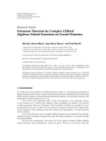
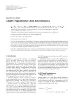
Figure 1: Estimation of the good detection probability for DVB-T
signals, mode 8k, with η
= 1/4 and an observation time equal to 50
milliseconds.
simulation of many realizations. Before describing these con-
texts, we describe one realization.
We have generated OFDM signals with the same mod-
ulation parameters as DVB-T signals [18]. We used the 8 k
mode, corresponding to N
= 8192 carriers where only the
first 6818 carriers are used to transmit data and pilots. Ac-
cording to [18], the sample rate is equal to T
c
= 1/8mi-
crosecond, and we have generated signals of 50 milliseconds.
Two cases have been considered for the cycle prefix length,
corresponding to η
= 1/4andη = 1/32.
For each realization, a simulated DVB-T discrete time
signal is passed through the DVB-T channel model described
in [17], and an i.i.d. centered Gaussian noise is added to the
output of this filter. The resulting signal is used as an input
to the detection algorithm.
Each context is defined by an SNR value and a value of
N
b
. We have evaluated the performances of the proposed al-
gorithm as the percentage of realizations where the criterion
excited by the simulated DVB-T signals satisfies the detection
test proposed in Section 3 with P
fa
= 2% over 1000 realiza-
tions.
The estimated good detection probabilities of the algo-
rithm are illustrated in Figure 1 for η
= 1/4 and in Figure 2
for η
= 1/32. Several choices of N
b
have been tested to illus-
trate the impact of this parameter on the performances of the
algorithm.
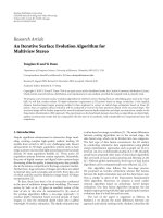
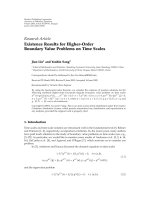
In both figures, the results show that whatever the value
of η is, the detection algorithm performances are improved
as long as N
b
is chosen to be lower than 1/η. Despite the loss
on the asymptotic mean value of the criterion, taking into
account the cycle frequencies leads to a significant improve-
ment on the detection performances.
Note that without taking into account the cycle frequen-
cies, the performances of the cyclic prefix detector proposed
Good detection probability
SNR
0
0.1
0.2
0.3
0.4
0.5
0.6
0.7
0.8
0.9
1
−15 −14 −13 −12 −11 −10 −9 −8 −7 −6 −5
N
b
= 0
N
b
= 1
N
b
= 2
N
b
= 3
N
b
= 4
N
b
= 5
N
b
= 6
N
b
= 7
Figure 2: Estimation of the good detection probability for DVB-T
signals, mode 8k, with η
= 1/32 and an observation time equal to
50 milliseconds.
by [14] do not fit with the requirement of the 802.22 WG
when η
= 1/32 since the good detection probability when
the SNR is close to
−10 dB is close to 70%. Thanks to our
algorithm, when taking into account 15 cycle frequencies
(N
b
= 7), the good detection probability remains close to
1uptoSNRof
−12 dB.
6. CONCLUSION
In this paper, we have proposed a detection algorithm based
on a cost function testing the cyclostationary property of the
OFDM signals. The noise and multipath channel impacts on
the proposed cost function have been theoretically analyzed.
Thanks to asymptotic results, a detection test has also been
proposed based on the false alarm probability, and some in-
dications on the choice of the N
b
have been given.
The evaluated performances of our detection algorithm
are illustrated in Figures 1 and 2. As shown, the proposed
detection algorithm has a good detection probability close to
1withanSNRof
−12 dB when η = D/N = 1/32. In the same
context, the detection algorithm proposed by [14]hasagood
detection probability close to 1 with an SNR of
−8dB.When
η
= 1/4, the proposed algorithm has a gain of 2 dB compared
to the algorithm of [14].
APPENDICES
A. PROOF OF THEOREM 2
As δf has no impact on the cost function, it can be neglected.
The signal z(u) then writes
z(u)
=
L−1
l=0
h(l)y(u −l)+σw(u). (A.1)
6 EURASIP Journal on Wireless Communications and Networking
Its cycle correlation coefficients are given by
R
(kα
0
)
z
(N) = lim
U→∞
1
U
U−1
u=0
E
z(u + N)z
∗
(u)
e
−2iπkα
0
u
. (A.2)
Using the mutual independence between the noise signal
w(u) and the signal of interest y(u), and the fact that the
noise signal is white, this coefficient is simplified to
R
(kα
0
)
z
(N)
=lim
U→∞
1
U
U−1
u=0
L
−1
l
1
=0
L
−1
l
2
=0
h
l
1
h
∗
l
2
E
y
u+N−l
1
y
∗
u−l
2
e
−2iπkα
0
=lim
U→∞
1
U
U−1
u=0
L
−1
l
1
=0
L
−1
l
2
=0
h
l
1
h
∗
l
2
R
y
u−l
2
, N +
l
2
−l
1
e
−2iπkα
0
.
(A.3)
The correlation function of y(n)isgivenby(5), and as-
suming that the channel impulse response satisfies 2L<N,
R
y
(u −l
2
, N +(l
2
−l
1
)) is simplified to R
y
(u −l
2
, N)δ(l
2
−l
1
).
Remark 3. The condition 2L<Nis not satisfied for the
DVB-T channel model given in [17]. Nevertheless, the co-
efficients vanish in an exponential way and can be neglected
when L>D
= N/32, the cyclic prefix size of DVB-T signals.
R
(kα
0
)
z
(N) then writes
R
(kα
0
)
z
(N) = lim
U→∞
1
U
U−1
u=0
L
−1
l=0
h(l)
2
R
y
(u −l, N)e
−2iπkα
0
.
(A.4)
Thanks to the Fourier decomposition of R
y
(u − l, N) (see
(6)), R
(kα
0
)
z
(N) also equals
R
(kα
0
)
z
(N)
= lim
U→∞
1
U
U−1
u=0
L
−1
l=0
h(l)
2
(N+D)/2
−1
k
2
=−(N+D)/2
R
(k
2
α
0
)
y
(N)e
2iπk
2
α
0
(u−l)
e
−2iπkα
0
=
L−1
l=0
h(l)
2
(N+D)/2
−1
k
2
=−(N+D)/2
R
(k
2
α
0
)
y
(N)e
−2iπk
2
α
0
l
lim
U→∞
1
U
U−1
u=0
e
2iπ(k
2
−k)α
0
u
.
(A.5)
As
|k
2
−k|α
0
< 1, we get the expected result:
R
(kα
0
)
z
(N) = R
(kα
0
)
y
(N)
L−1
l=0
h(l)
2
e
−2iπkα
0
l
. (A.6)
B. PROOF OF THEOREM 3
This proof is based on the model of the DVB-T channels
given by [17]. The channel coefficients are randomly cho-
sen and uncorrelated, that is,
E{h(l)h
∗
(k)}=0, for all l
/
= k.
Each channel coefficient h
l
is randomly chosen according to a
zero-mean complex Gaussian distribution with the variance
given by
E
h(0)
2
=
c
0
+ c
1
1 −e
−T
c
/τ
,
E
h(k)
2
=
c
1
1 −e
−T
c
/τ
e
−k(T
c
/τ)
, ∀k ≥ 1.
(B.1)
c
0
and c
1
are randomly chosen coefficients. c
0
+ c
1
defines
the channel attenuation or channel power, and the ratio c
0
/c
1
is referred to as the K factor. When K grows to infinity, the
channel impulse response corresponds to an LOS scenario
(flat fading channel). Otherwise, K is the ratio between the
direct path and the other one. For the NLOS scenarios, K in
dB takes values in the set (
−∞;8] dB. τ is the delay spread
and takes values in the set [0.1, 0.8] microsecond. We remind
that for DVB-T signals, T
c
equals 0.125 microsecond, making
the ratio T
c
/τ close to 1.
For each value of k, the term
E
h
|
L−1
l
=0
|h(l)|
2
e
−2iπlkα
0
|
2
writes
E
h
L−1
l=0
h(l)
2
e
−2iπlkα
0
2
=
l
1
,l
2
E
h
h
l
1
2
h
l
2
2
e
−2iπ(l
1
−l
2
)kα
0
.
(B.2)
In terms of cumulants, since h(l)iscircular,
E
h
{|h(l
1
)|
2
|h(l
2
)|
2
}
writes
E
h
h
l
1
2
h
l
2
2
=
cum
h
l
1
, h
∗
l
1
, h
l
2
, h
∗
l
2
+ E
h
h
l
1
2
E
h
h
l
2
2
+
E
h
h
l
1
h
∗
l
2
2
.
(B.3)
As h(l) is Gaussian, the fourth-order cumulant van-
ishes. With the channel coefficient being uncorrelated,
|E{h(l
1
)h
∗
(l
2
)}|
2
= δ(l
1
−l
2
)|E
h
|h(l
1
)|
2
|
2
.
E
h
|
L−1
l
=0
|h(l)|
2
e
−2iπlkα
0
|
2
then writes in terms of the
second-order moment as
E
h
L−1
l=0
h(l)
2
e
−2iπlkα
0
2
=
L−1
l=0
E
h
h(l)
2
e
−2iπlkα
0
2
+
L−1
l=0
E
h
h(l)
2
2
.
(B.4)
Thanks to (B.1), the first r.h.s. term writes
L−1
l=0
E
h
|h(l)|
2
e
−2iπlkα
0
2
=
c
0
+ c
1
1 −e
−T
c
/τ
1 −e
−2iπkα
0
−T
c
/τ
1 −e
−2iLπkα
0
−L(T
c
/τ)
2
.
(B.5)
When L is large enough, 1
−e
−2iLπkα
0
−L(T
c
/τ)
→ 1. Concerning
the term 1
− e
−2iπkα
0
−T
c
/τ
,asα
0
= 1/(N + D)andk ≤ N
b
=
N/D = 1/η, kα
0
< 1/2ηN. Hence, when N grows to infinity,
1
−e
−2iπkα
0
−T
c
/τ
→ 1−e
−T
c
/τ
. When N and L grow to infinity,
the first r.h.s. term of (B.4) tends to
|
L−1
l
=0
E
h
|h(l)|
2
|
2
.
Pierre Jallon 7
These results led to the expected result: when N and L
grow to infinity, (B.4) tends to
E
h
L−1
l=0
h(l)
2
e
−2iπlkα
0
2
−→ Λ
h
=
L−1
l=0
E
h
h(l)
2
2
+
L−1
l=0
E
h
h(l)
2
2
.
(B.6)
C. PROOF OF THEOREM 4
If H
0
holds, y(n) = σ
2
w(n) is a centered i.i.d. Gaussian noise.
The estimates of its cycle coefficients are given by
R
(kα
0
)
y
(N) =
1
U
U−1
u=0
y(u + N)y
∗
(u)e
−2iπkα
0
u
,(C.1)
where U is the observation time. Thanks to the law of large
number,
R
(kα
0
)
y
(N) is asymptotically normal. Its mean is given
by
E
R
(kα
0
)
y
(N)
=
1
U
U−1
u=0
E
y(u + N)y
∗
(u)
e
−2iπkα
0
u
= R
(kα
0
)
y
(N).
(C.2)
As y is a Gaussian i.i.d. signal,
E{
R
(kα
0
)
y
(N)}=0.
We now focus on the asymptotic covariance:
E
R
(k
1
α
0
)
y
(N)
R
(k
2
α
0
)
y
(N)
∗
=
1
U
2
U
−1
u
1
,u
2
=0
E
y
u
1
+N
y
∗
u
1
y
∗
u
2
+N
y
u
2
e
−2iπα
0
(k
1
u
1
−k
2
u
2
)
.
(C.3)
The fourth-order moment is written in terms of the cumu-
lant as
E
y
u
1
+ N
y
∗
u
1
y
∗
u
2
+ N
y
u
2
=
cum
y
u
1
+ N
, y
∗
u
1
, y
∗
u
2
+ N
y
u
2
+ E
y
u
1
+ N
y
∗
u
1
E{
y
∗
u
2
+ N)y
u
2
+ E
y
u
1
+ N
y
u
2
E{
y
∗
u
2
+ N
y
∗
u
1
+ E
y
u
1
+ N
y
∗
u
2
+ N
E{
y
∗
u
1
y
u
2
.
(C.4)
As the noise is Gaussian, the fourth-order cumulant vanishes.
The second term equals R
y
(u
1
, N)(R
y
(u
2
, N))
∗
which also
vanishes since the signal is i.i.d. The third term equals 0 since
the signal is circular at order 2. The asymptotic covariance
depends hence only on the third term and is simplified to
E
R
(k
1
α
0
)
y
(N)
R
(k
2
α
0
)
y
(N)
∗
=
1
U
2
U
−1
u
1
,u
2
=0
E
y
u
1
+ N
y
∗
u
2
+ N
×E
y
∗
u
1
y
u
2
e
−2iπα
0
(k
1
u
1
−k
2
u
2
)
.
(C.5)
Using the i.i.d. property of the noise signal, this expression
vanishes if u
1
/
= u
2
.Ifu
1
= u
2
, E{y(u
1
+ N)y
∗
(u
2
+ N)}=
E{
y
∗
(u
1
)y(u
2
)}=σ
2
.Weget
E
R
(k
1
α
0
)
y
(N)
R
(k
2
α
0
)
y
(N)
∗
=
σ
4
1
U
2
U
−1
u=0
e
−2iπα
0
u(k
1
−k
2
)
.
(C.6)
The asymptotic variance
E|
R
(kα
0
)
y
(N)|
2
is then equiva-
lent to σ
4
/U.Ifk
1
/
= k
2
, the asymptotic covariance
E{
R
(k
1
α
0
)
y
(N)(
R
(k
2
α
0
)
y
(N))
∗
} is equivalent to
E
R
(k
1
α
0
)
y
(N)
R
(k
2
α
0
)
y
(N)
∗
=
σ
4
U
2
e
−iπα
0
(U−1)(k
1
−k
2
)
sin
πα
0
U
k
1
−k
2
sin
πα
0
k
1
−k
2
.
(C.7)
When U grows to
∞, UE{
R
(k
1
α
0
)
y
(N)(
R
(k
2
α
0
)
y
(N))
∗
} tends to
0. Note that the
R
(k
1
α
0
)
y
(N)and
R
(k
2
α
0
)
y
(N) can be considered
as uncorrelated only if U>1/
|k
1
−k
2
|.
C.1. Proof of Corollary 1
With the estimate of the cycle correlation coefficients being
asymptotic uncorrelated Gaussian variable, the probability
density function of
2N
b
+1
σ
4
U
J
N
b
=
N
b
k=−N
b
U
σ
4
R
(kα
0
)
y
(N)
2
(C.8)
is a χ
2
law with 2(2N
b
+ 1) degrees of freedom. The expected
result can then be deduced.
C.2. Proof of Corollary 2
Thanks to the previous results, we also know that
E
2N
b
+1
σ
4
U
J
N
b
=
2N
b
+1
(C.9)
or equivalently that
E{
J(N
b
)}=U/σ
4
. Concerning the
asymptotical covariance, we get
E
2N
b
+1
σ
4
U
J
N
b
−E
2N
b
+1
σ
4
U
J
N
b
2
=2N
b
+1
(C.10)
or equivalently
E|
J(N
b
) −E{
J(N
b
)}|
2
= σ
8
/(U
2
(2N
b
+ 1)).
D. PROOF OF THEOREM 6
To give some results on the statistical behavior of
J
y
(N
b
), we
first give some results on the behavior of the cycle coefficients
estimator
R
(kα
0
)
y
(N).
D.1. Statistical behavior of
R
(kα
0
)
y
(N)
If H
1
holds, y(n) =
E
s
s
a
(nT
c
)+σw(n) is a centered i.i.d.
Gaussian noise. To evaluate the statistical behavior of J
y
(N
b
),
we first introduce the vector R
y
defined as
R
y
=
R
(−N
b
α
0
)
y
(N), , R
(0)
y
(N), , R
(N
b
α
0
)
y
(N)
T
(D.1)
8 EURASIP Journal on Wireless Communications and Networking
and
R
y
as its estimate. Thanks to the law of large number,
R
y
is asymptotically normal. For each component, its mean is
given by
E
R
(kα
0
)
y
(N)
=
1
U
U−1
u=0
E
y(u + N)y
∗
(u)
e
−2iπkα
0
u
= R
(kα
0
)
y
(N).
(D.2)
Only the OFDM signal s
a
(t) contributes to this term which
does not vanish. To compute the estimator variance, we in-
troduce the covariance matrix as Γ
= lim
U→∞
UE{(
R
y
−
R
y
)(
R
y
−R
y
)
H
}. Its coefficients are given by
[Γ]
k,l
= lim
U
UE
R
(−N
b
+kα
0
)
y
(N)
R
(−N
b
+lα
0
)
y
(N)
∗
−
UR
(−N
b
+kα
0
)
y
(N)
R
(−N
b
+lα
0
)
y
(N)
∗
.
(D.3)
Similarly to the previous proof, we get after some calculations
E
R
(−N
b
+kα
0
)
y
(N)
R
(−N
b
+lα
0
)
y
(N)
∗
=
R
(−N
b
+kα
0
)
y
(N)
R
(−N
b
+lα
0
)
y
(N)
∗
+
1
U
2
u,v
R
y
(u + N, v)R
∗
y
(u, v)e
−2iπα
0
(k−l)u
.
(D.4)
Hence,
[Γ]
k,l
= lim
U
1
U
u,v
R
y
(u + N, v)R
∗
y
(u, v)e
−2iπα
0
(k(u+v)−lu)
.
(D.5)
R
y
(u, v) vanishes when v
/
= 0andv
/
=±N.Ifv = 0, R
∗
y
(u,0)
does not depend on u.Hence,
lim
U
1
U
u
R
y
(u+N,0)R
∗
y
(u,0)e
−2iπα
0
(k−l)u
=
E
s
+σ
2
2
δ(k−l).
(D.6)
When v is equal to
±N, the expression is more complex. We
will write it as
lim
U
1
U
u
R
y
(u+N,±N)R
∗
y
(u,±N)e
−2iπα
0
((k−l)u−k(±N))
=O
E
2
s
.
(D.7)
The matrix Γ has then the following form:
Γ
=[O(E
2
s
)]+
⎡
⎢
⎢
⎢
⎢
⎣
(E
s
+ σ
2
)
2
+O(E
2
s
)0 0
0
.
.
.
0
00(E
s
+σ
2
)
2
+O(E
2
s
)
⎤
⎥
⎥
⎥
⎥
⎦
.
(D.8)
D.2. Statistical behavior of
J
y
(N
b
)
To evaluate the statistical behavior of
J
y
, we first write this
function in terms of
R
y
:
J
y
=
1
2N
b
+1
R
H
y
R
y
. (D.9)
As
R
y
2
is positive, we deduce that
√
U(
J
y
− J
y
)converges
in law to N (0, 4Σ)(see[19] for more details). The matrix Σ
is given by
Σ
=
1
2N
b
+1
2
R
H
y
R
T
y
ΓΓ
c
Γ
∗
c
Γ
∗
⎡
⎣
R
y
R
∗
y
⎤
⎦
, (D.10)
where R
∗
y
is the conjugate of R
y
and Γ
c
= lim
U→∞
UE{(
R
y
−
R
y
)(
R
y
−R
y
)
T
}.
Remark 4. To be proved, the result of Theorem 6 concern-
ing the mean behavior of
J only requires some calculations
considering lim
U→∞
U(E{
J
y
}−J
y
).
The coefficients Γ
c
are given by
Γ
c
k,l
= lim
U
UE
R
(−N
b
+kα
0
)
y
(N)
R
(−N
b
+lα
0
)
y
(N)
−
UR
(−N
b
+kα
0
)
y
(N)R
(−N
b
+lα
0
)
y
(N).
(D.11)
After some calculations, we also get
Γ
c
k,l
= lim
U
1
U
u
1
,u
2
R
y
u
1
, u
1
−u
2
+ N
×
R
∗
y
u
2
, −u
1
+ u
2
+ N
e
−2iπα
0
(ku
1
+lu
2
)
.
(D.12)
[Γ
c
]
k,l
does not vanish only when u
1
= u
2
, which gives
Γ
c
k,l
= lim
U
1
U
u
R
y
(u,+N)R
∗
y
(u, N)e
−2iπα
0
(k+l)u
= O
E
2
s
.
(D.13)
The matrix Γ
c
has then the following form: Γ
c
= [O(E
2
s
)].
The matrix
ΓΓ
c
Γ
∗
c
Γ
∗
is hence simplified to
ΓΓ
c
Γ
∗
c
Γ
∗
=
2
O
E
2
s
+
⎡
⎢
⎢
⎢
⎢
⎣
E
s
+σ
2
2
+O
E
2
s
00
0
.
.
.
0
00
E
s
+σ
2
2
+O
E
2
s
⎤
⎥
⎥
⎥
⎥
⎦
,
(D.14)
which leads to the expected result when E
s
σ
2
(i.e., the
terms O(E
2
s
) are neglected):
E
J
y
−J
y
2
=
β
2N
b
+1
. (D.15)
Pierre Jallon 9
E. PROOF OF THEOREM 7
The cycle coefficients of the signal y(n)
=
E
s
s
a
(uT
c
)+σw(u)
are given by
R
(kα
0
)
y
(N) = lim
U→∞
1
U
U−1
u=0
E
y(u + N)y
∗
(u)
e
−2iπukα
0
=
E
s
N + D
N+D−1
u=N
e
−2iπukα
0
.
(E.1)
As α
0
= 1/(N +D), the r.h.s term is simplified to the expected
result:
R
(kα
0
)
y
(N) =
e
−iπ(k/(N+D))(2N+D−1)
N + D
sin
π(D/(N + D)
k
sin
π
k/(N + D)
.
(E.2)
REFERENCES
[1] J. Mitola, Cognitive radio: an integrated agent architecture for
software defined radio, Ph.D. thesis, Royal Institute of Technol-
ogy, Stockholm, Sweden, 2000.
[2] R. Etkin, A. Parekh, and D. Tse, “Spectrum sharing for unli-
censed bands,” IEEE Journal on Selected Areas in Communica-
tions, vol. 25, no. 3, pp. 517–528, 2007.
[3] Shared Spectrum Company, “Spectrum occupancy report for
new york city during the republican convention August-
September, 2004,” in ICC, 2006.
[4] P. Kolodzy, “Spectrum policy task force: findings and recom-
mendations,” in Proceedings of the International Symposium on
Advanced Radio Technologies (ISART ’03), Boulder, Colo, USA,
March 2003.
[5] Federal Communications Commission, “FCC 04-113—
unlicensed operation in the TV broadcast bands,” in ET
Docket No. 04-186, May 2004.
[6] G. Chouinard, “IEEE P802.22 wireless RANs—WRAN keep-
out region,” June 2006.
[7] C. Cordeiro, K. Challapali, D. Birru, and N. Sai Shankar, “IEEE
802.22: an introduction to the first wireless standard based on
cognitive radios,” JournalofCommunications,vol.1,no.1,pp.
38–47, 2006.
[8] H. Urkowitz, “Energy detection of unknown deterministic sig-
nals,” Proceedings of the IEEE, vol. 55, no. 4, pp. 523–531, 1967.
[9] S. V. Schell, “An overview of sensor-array processing for cyclo-
stationary signals,” in Cyclostationarity in Communication and
Signal Processing, W. A. Gardner, Ed., pp. 168–239, IEEE Press,
New York, NY, USA, 1994.
[10] D. Dehay and H. L. Hurd, “Representation and estimation for
periodically and almost periodically correlated random pro-
cesses,” in Cyclostationarity in Communications and Signal Pro-
cessing, W. A. Gardner, Ed., IEEE Press, New York, NY, USA,
1993.
[11] H. L. Van Trees, Detection, Estimation, and Modulation Theory:
Radar-Sonar Signal Processing and Gaussian Signals in Noise—
Part III, John Wiley & Sons, New York, NY, USA, 2nd edition,
2001.
[12] A. V. Dandawate and G. B. Giannakis, “Statistical tests for
presence of cyclostationarity,” IEEE Transactions on Signal Pro-
cessing, vol. 42, no. 9, pp. 2355–2369, 1994.
[13] M.
¨
Oner and F. Jondral, “On the extraction of the channel allo-
cation information in spectrum pooling systems,” IEEE Jour-
nal on Selected Areas in Communications,vol.25,no.3,pp.
558–565, 2007.
[14] Huawei Technologies UESTC, “IEEE P802.22 wireless RANs—
sensing scheme for DVB-T,” November 2006.
[15] P. Liu, B B. Li, Z Y. Lu, and F K. Gong, “A blind time-
parameters estimation scheme for OFDM in multi-path chan-
nel,” in Proceedings of International Conference on Wireless
Communications, Networking and Mobile Computing (WCNM
’05), vol. 1, pp. 242–247, Wuhan, China, September 2005.
[16] H. Ishii and G. W. Wornell, “OFDM blind parameter identi-
fication in cognitive radios,” in Proceedings of the 16th IEEE
International Symposium on Personal, Indoor and Mobile Ra-
dio Communications ( PIMRC ’05), vol. 1, pp. 700–705, Berlin,
Germany, September 2005.
[17] E. Sofer and G. Chouinard, “IEEE P802.22 wireless RANs—
WRAN channel modeling,” September 2005.
[18] ETSI, “Digital videl broadcasting (DVB) framing structure,
channel coding and modulation for digital terrestrial televi-
sion,” November 2004.
[19] R. A. Davis and P. J. Brockwell, Time Series: Theory and Meth-
ods, Springer Series in Statistics, Springer, New York, NY, USA,
1998.