Báo cáo hóa học: " Research Article Audio Watermarking through Deterministic plus Stochastic Signal Decomposition" pot

Hindawi Publishing Corporation
EURASIP Journal on Information Security
Volume 2007, Article ID 75961, 12 pages
doi:10.1155/2007/75961
Research Article
Audio Watermarking through Deterministic p lus
Stochastic Signal Decomposition
Yi-Wen Liu
1, 2
and Julius O. Smith
1
1
Center for Computer Research in Music and Acoustics (CCRMA), Stanford University, Palo Alto, CA 94305, USA
2
Boys Town National Research Hospital, 555 North 30th Street, Omaha, NE 68131, USA
Correspondence should be addressed to Yi-Wen Liu,
Received 1 May 2007; Revised 10 August 2007; Accepted 1 October 2007
Recommended by D. Kirovski
This paper describes an audio watermarking scheme based on sinusoidal signal modeling. To embed a watermark in an original
signal (referred to as a cover signal hereafter), the following steps are taken. (a) A short-time Fourier transform is applied to the
cover signal. (b) Prominent spectral peaks are identified and removed. (c) Their frequencies are subjected to quantization index
modulation. (d) Quantized spectral peaks are added back to the spectrum. (e) Inverse Fourier transform and overlap-adding
produce a watermarked signal. To decode the watermark, frequencies of prominent spectral peaks are estimated by quadratic
interpolation on the magnitude spectrum. Afterwards, a maximum-likelihood procedure determines the binary value embedded in
each frame. Results of testing against lossy compression, low- and highpass filtering, reverberation, and stereo-to-mono reduction
are reported. A Hamming code is adopted to reduce the bit error rate (BER), and ways to improve sound quality are suggested as
future research directions.
Copyright © 2007 Y W. Liu and J. O. Smith. This is an open access article distributed under the Creative Commons Attribution
License, which permits unrestricted use, distribution, and reproduction in any medium, provided the original work is properly
cited.
1. INTRODUCTION

The audio watermarking community has successfully
adopted frequency-domain masking models standardized by
MPEG. Below the masking threshold, a spread spectrum wa-
termark (e.g., [1, 2]) distributes its energy, and the same
threshold also sets a limit to the step size of quantization in
informed watermarking [3]. Nevertheless, subthreshold per-
turbation is not the only way to generate perceptually similar
sounds. Alternatively, a signal comprised of a large number of
samples can be modeled with fewer variables called param-
eters [4]. Then, a watermark can be embedded in the signal
through small perturbation in the parameters [5].
Audio signals can be parameterized while retaining sur-
prisingly high sound quality. A classic parametric model is
linear prediction [6], which enables speech to be encoded in
filter coefficients and excitation source parameters [7]. An-
other model is to represent a tonal signal as a sparse sum
of time-varying sinusoids [8, 9]. Although developed sep-
arately, predictive modeling and sinusoidal modeling have
been used jointly [10]. A signal is modeled as a sum of si-
nusoids, and the residual signal that does not fit well to the
model is parameterized by linear prediction. This hybrid sys-
tem is referred to as being “deterministic plus stochastic”
(D+S). The D component refers to the sinusoids, and the S
component refers to the residual because it lacks tonal qual-
ity, therefore sounding like filtered noise. D+S decomposi-
tion was refined by Levine [11] by further decomposing the S
component into a quasistationary “noise” part and a rapidly
changing “transient” part. Levine’s decomposition was given
the name sines + noise + transients and considered as an
efficient and expressive audio coding scheme. The develop-

ment in D+S modeling has culminated in its endorsement
by MPEG-4 as part of the audio coding standard [12].
In audio watermarking, meanwhile, the flexibility of D+S
decompositions has brought forth a few novel schemes in
recent years. Using Levine’s terminology, watermarks have
been embedded in two of the three signal components—in
the transient part through onset time quantization, and in
the sinusoids through phase quantization or frequency ma-
nipulation.
Embedding in the transients relies on an observation that
the locations of a signal’s clear onsets in its amplitude enve-
lope are invariant to common signal processing operations
2 EURASIP Journal on Information Security
Audio in
Blackman
window
STFT
Peak
detection
Peak
tracking
Wat ermar k
0100101
F-QIM
Sinusoidal
synthesis
Wat ermar ked
sinusoids
−
+

I-FFT OLA
Residual
Previous
frame
Energy
ratio
SRR
< 0.5 ?
> 1.5 ?
Transient Y/N
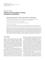
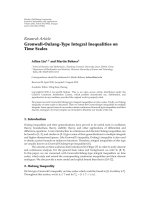
Figure 1: Signal decomposition and watermark embedding. Highlighted areas indicate (from top to bottom) the sinusoid processing mod-
ules, the residual computation modules, and the transient detection logic, respectively.
[13]. Such onsets, sometimes referred to as salient points,can
be identified by wavelet decomposition [14]andquantized
in time to embed watermarks; Mansour and Tewfik [15]re-
ported robustness to MPEG compression (at 112kbps/ch)
and lowpass filtering (at 4 kHz), and their system sustained
up to 4% of time-scaling modification with a probability of
error less than 7%. Repetition codes were applied to achieve
reliable data hiding at 5 bps (bits per second).
Phase quantization watermarking was first proposed by
Bender et al. [16]. For each long segment of a cover signal,
the phase at 32–128 frequency bins of the first short frame
was replaced by
±π/2, representing the binary 1 or 0, re-
spectively. In all of the frames to follow, the relative phase
relation was kept unchanged. More recently, Dong et al.[17]
proposed a phase quantization scheme which assumes har-
monic structure of speech signals. The absolute phase of each
harmonic was modified by Chen and Wornell’s quantization

index modulation [18](QIM)withastepsizeofπ/2, π/4,
or π/8. About 80 bps of data hiding was reported, robust to
80 kbps/ch of MP3 compression with a BER of approximately
1%.
Although phase quantization is shown as being robust to
perceptual audio compression, human hearing is not highly
sensitive to phase distortion, as argued by Bender et al. [16].
Thus, an attacker has the freedom to use imperceptible fre-
quency modulation and steer the absolute phase of a compo-
nent arbitrarily, thus defeating phase quantization schemes.
Therefore, in the present work, we seek to embed a water-
mark not in the absolute phase of a component, but in its
rate of change, the instantaneous frequency.
At first, audio watermarking by manipulating the cover
signal’s frequency was inspired by echo-hiding [16]. Petrovic
[19] observed that an echo is a “replica” of the cover signal
placed at a delay and the echo becomes transparent if it is
sufficiently attenuated. He then attempted to place an atten-
uated replica at a shifted frequency to encode hidden infor-
mation, but he did not disclose details of watermark decod-
ing. Succeeding Petrovic’s work, Shin et al. [20] utilized pitch
scaling of up to 5% at mid frequency (3-4 kHz) for water-
mark embedding. Data hiding of 25 bps robust to 64 kbps/ch
of audio compression were reported with BER <5%. A year
later, we achieved 50 bps of data hiding by QIM in the fre-
quency of sinusoidal models, but the algorithm only applied
to synthetic sounds [5]. Independently, Girin and Marchand
[21] studied frequency modulation for audio watermarking.
In speech signals, surprisingly, frequency modulation in the
6th harmonic or above was found imperceptible up to a de-

viation of 0.5 times of the fundamental frequency. Based on
this observation, transparent watermarking at 150 bps was
achieved by coding 0 and 1 with positive and negative fre-
quency deviations, respectively.
The watermarking scheme presented in this paper also
induces frequency shifts to the cover signal but it differs from
previous work in a few ways. First, the cover signal is re-
placed by, instead of being superposed w ith, the replica. This is
achieved through sinusoidal modeling, spectral subtraction,
and QIM in frequency (hereafter referred to as F-QIM). Sec-
ond, the scale of frequency quantization, based on studies of
pitch sensitivity in human hearing, is about an order of mag-
nitude smaller than that described by Shin et al. [20]and
Girin and Marchand [21]. The watermark decoding there-
fore requires unprecedented accuracy of frequency estima-
tion. To this end, a frequency estimator that approaches the
Cram
´
er-Rao bound (CRB) is adopted. Third, as an extension
to our previous work [5, 22], the new scheme is not limited to
synthetic signals. Design of the new scheme is described next.
Afterwards, in Section 3,robustnessisevaluated,andresults
from a pilot listening test are reported. Rooms for improve-
ment are pointed out in Section 4. Particularly, watermark
security of the F-QIM scheme remains to be addressed. In
this regard, this paper should be viewed as a proof of concept
rather than a complete working solution.
2. METHODS
The watermark encoding process is based on the decompo-
sition of a cover signal into sines + noise + transients. As

shown in Figure 1, initially, the spectrum of the cover sig-
nal is computed by the short-time Fourier transform (STFT).
If the current frame contains a sudden rise of energy and
the sine-to-residual energy ratio (SRR) is low, it is labeled
transient and passed to the output unaltered. Otherwise,
Y W.LiuandJ.O.Smith 3
prominent peaks are detected and represented by sinusoidal
parameters. The residual component is computed by remov-
ing all the prominent peaks from the spectrum, transforming
the spectrum back to the time domain through inverse FFT
(I-FFT), and then overlap-adding (OLA) the frames in time.
Parallel to this, a peak tracking unit memorizes sinusoidal
parameters from the past and links peaks across frames to
form trajectories. The watermark is embedded in the trajec-
tories via QIM in frequency. The signal that takes quantized
trajectories to synthesize consists of watermarked sinusoids.
In this paper, a watermarked signal is defined as the sum of
the watermarked sinusoids, the residual, and the unaltered
transients. Details of each building block are described next.
2.1. Implementing D+S decomposition
Window selection
To compute STFT, the Blackman window [23]oflength
L
= 2N is adopted, N = 1024. Compared to the more com-
monly used Hann window, the Blackman window is better in
terms of its side lobe rejection (57 versus 31 dB) and spectral
roll-off rate (18 versus 12 dB per octave). Thus, the residual
components after spectral subtraction (to be described) are
masked better using the Blackman window.
Calculating the masking curve

Only unmasked peaks are used for watermark embedding.
The masking curve is computed via a spreading function
ψ(z) that approximates the pure-tone excitation pattern on
the human basilar membrane [24]:
dψ
dz
=
⎧
⎪
⎪
⎪
⎪
⎪
⎨
⎪
⎪
⎪
⎪
⎪
⎩
0, z
0
− 0.5 ≤ z ≤ z
0
+0.5,
27, z<z
0
− 0.5,
−27, z>z
0

+0.5, Λ ≤ 40,
−27 + K(Λ −40), z>z
0
+0.5, Λ > 40,
(1)
where Λ is the sound pressure level (SPL) in dB (re: 2
×
10
−5
Pa), K = 0.37, z
0
is the pure tone’s frequency in Barks
[25], and z is the critical band rate, also in Barks, at other fre-
quencies. ψ(z
0
) = 0. Note that SPL is a physically measurable
quantity. To align it with digital signals, a pure tone at the
maximum amplitude (e.g., 1 for compatibility with MAT-
LAB’s wavread function) is arbitrarily set equal to 100 dB
SPL. The masking level M(z)isgivenby
M(z)
= Λ − Δ(z
0
)+ψ(z), (2)
where the offset Δ
= (14.5+z
0
)dB[26].
1
1

The spreading function in (1) is similar to MPEG psychoacoustic model
1 (in ISO/IEC 11172-3). They share a few common features. First, the
spreading function rolls off faster on the low-frequency side than on the
high-frequency side. Second, the slope on the high-frequency side de-
creases as the sound level increases. However, what this psychoacoustic
model lacks is the ability to differentiate between tonal and nontonal
maskerssoastosetΔ(z
0
) accordingly. In (2), this model always assumes
that maskers are tonal. Readers interested in calculation of a tonal index
can refer to [27, Chapter 11].
To e x p r e s s M(z) in units of power per frequency bin, the
following normalization is necessary [28]:
M
2
k
=
10
M(z)/10
N(z)
,(3)
where N(z) is the equivalent number of FFT bins within a
critical bandwidth (CBW) [25]centeredatz
= z(kΩ), with
kΩ
= k(2π/N
FFT
) being the frequency of the kth bin.
When more than one tone is present, the overall masking
curve σ

2
(kΩ) is set as the maximum of the spreading func-
tions and the threshold in quiet I
0
( f ):
σ
2
(kΩ) = max

M
2
1,k
, M
2
2,k
, , M
2
j,k
,10
I
0
(kΩ)/10

,(4)
where M
j,k
denote the masking level at frequency bin k due to
the presence of tone j,andI
0
( f ) is calculated using Terhardt’s

approximation [29]:
I
0
( f )/dB = 3.64 f
−0.8
− 6.5e
−0.6( f −3.3)
2
+10
−3
f
4
,(5)
where f is in the unit of kHz. In this paper, a peak is consid-
ered “prominent” if its intensity is higher than the masking
curve. To carry a watermark, prominent peaks will be sub-
tracted from the spectrum and then added back at quantized
frequencies.
Spectral interpolation and subtraction
Sinusoidal modeling parameters are estimated via a
quadratic interpolation of the log-magnitude FFT (QIFFT)
[30]. Blackman windowed signals of length 2048 are first
zero-padded to a length of 2
14
before FFT. Denote the
2
14
-length discrete spectrum S
k
= S(kΩ), Ω = 2π/2

14
. Any
peak such that


S
k


>


S
k+1


and


S
k


>


S
k−1



is associated
with frequency and amplitude estimates given by
ω =

k +
1
2
a
−
− a
+
a
−
− 2a + a
+

Ω,
log

A = a −
1
4


ω
Ω
− k


a

−
− a
+

− C,
(6)
where a
−
= log


S
k−1


, a
+
= log


S
k+1


, a = log


S
k



,
and C
= log(

N
n=−N
w
B
[n]) are a normalization factor, with
w
B
[n] being the Blackman window. Denote q = (ω/Ω) − k.
The phase estimate is given by linear interpolation:

φ = ∠S
k
+ q

∠S
k+1
− ∠S
k

. (7)
The sinusoid parameterized with
{

A, ω,


φ} can be re-
moved by spectral subtraction,asdescribedbelow.
Step 0. Initialize the sum spectrum

S(ω) = 0 and denote

S
k
=

S(kΩ).
4 EURASIP Journal on Information Security
Step 1. For each peak, fit the main lobe of the Blackman win-
dow transform W(ω)at
ω,scaleitby

Aexp( j

φ),
2
and denote
the scaled and shifted main lobe of the window as

W(ω) =
⎧
⎪
⎨
⎪
⎩


Ae
j

φ
W(ω − ω)if


ω − ω


≤
3
2π
L
,
0, otherwise.
(8)
Step 2. Denote

W
k
=

W(kΩ) and update

S
k
by

S

k
+

W
k
.
Step 3. Take the next prominent peak and repeat steps 1 and
2 until all prominent peaks are processed; and towards the
end,

S
k
becomes the spectrum to be subtracted.
Step 4. Define the residual spectrum R
k
as follows:
R
k
=

S
k
−

S
k
if


S

k
−

S
k


<


S
k


,
S
k
, otherwise.
(9)
The if condition in (9) guarantees that the residual spec-
trum is smaller than the signal spectrum everywhere, in
terms of its magnitude.
2.2. Residual and transient processing
Inaudible portion of the residual is removed by setting R
k
to
zero if
|R
k
|

2
is below the masking curve. Then, inverse FFT is
applied to obtain a residual signal r of the length N
FFT
. Due
to concerns that will be discussed later regarding perfect re-
construction, r is shaped in the time domain according to
r
sh
[n] = r[n]

w
H
[n]
w
B
[n]

, (10)
where w
H
[n] denotes Hann window of length N.Then,
across frames, r
sh
[n] is overlap-added with a hop of length
h
= N/2 to form the final residual signal r
OLA
[n]:
r

OLA
[n] =
∞

m=1
r
sh
m
[n −mh], (11)
where the subscript m is an index pointing to the frame cen-
teredaroundtimen
= mh.
Regions of rapid transients need to be identified and
treated with caution so as to avoid pre-echoes, which occur
when the short-time phase spectrum of a rapid onset is mod-
ified. If a pre-echo extends beyond the range of the onset’s
backward masking [25], it becomes an audible artifact. To
avoid pre-echoes, in the current study, regions of rapid on-
sets are kept unaltered. A frame is labeled “transient” if all of
the following conditions are true.
(i) The sines-to-residual energy ratio in the current frame
is less than 5.0.
2
For convenience of discussion, assume that the normalization factor is
C
= 0.
6k
5k
4k
3k

2k
1k
0
Frequency (Hz)
0.1 0.2 0.3 0.4 0.5 0.6 0.7 0.8 0.9
Time (s)
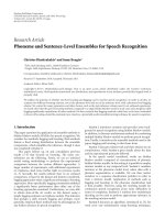
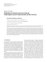
Figure 2: Frequency trajectories extracted from a recording of Ger-
man female speech, overlaid on its spectrogram. Onsets of trajecto-
ries are marked with dots. Arrows point to transient regions, where
peak detection is temporarily disabled.
(ii) The energy ratio of the current frame to the previous
frame is greater than 1.5.
(iii) There is at least a peak greater than 30 dB SPL between
2 and 8 kHz.
When all three criteria are met, spectral subtraction and wa-
termark embedding are disabled for 2048 samples around the
current frame. The signal fades in and out of the transient re-
gion using Hann window of length 1024 with 50% overlap.
2.3. Watermarking the sinusoids
Peak tracking
Denote the estimated frequencies of the peaks as
{ω

j
} and
{ω
j
} at previous and current frames, respectively. The fol-
lowing procedure connects peaks across the frame boundary.
Step 1. For each peak j in the current frame, find its closest

neighbor i(j) from the previous frame; i(j)
= arg min
k
|ω

k
−
ω
j
|, and connect peak i(j) of the previous frame to peak j of
the current frame.
Step 2. If a connection has a frequency slope greater than 20
barks per second, break the connection and label peak j of
the current frame as an onset to a new trajectory.
Step 3. If a peak i
0
in the previous frame is connected to more
than one peak in the current frame, keep only the connec-
tion with the smallest frequency jump, and mark all the other
peaks j such that i(j)
= i
0
as onsets to new trajectories.
A trajectory starts at an onset and ends whenever the
connection cannot continue. Trajectories extracted from a
recording of German female speech are shown in Figure 2.
Y W.LiuandJ.O.Smith 5
Sinusoidal synthesis
For each trajectory k,letφ
(k)

0
denote the initial phase, {A
km
}
its amplitude envelope, and {ω
km
} its frequency envelope. A
window-based synthesis can be written as
s
total
[n] =

k

m
A
km
w[n − mh]cos

φ
(k)
m
+ ω
km
(n −mh)

,
(12)
where the phase φ
(k)

m
is updated as follows:
φ
(k)
m
= φ
(k)
m
−1
+

ω
k,m−1
+ ω
km
2

h. (13)
In (12), the window w[n] needs to satisfy a perfect recon-
struction condition
∞

m=−∞
w[n − mh] = 1 ∀n. (14)
To be consistent with residual postprocessing in (10), the
Hann window is adopted in (12).
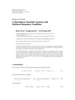
Designing frequency quantization codebooks
Frequency parameters
{ω
km

} in (12)arequantizedtoem-
bed a watermark. The just noticeable difference in frequency,
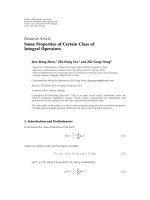
or frequency limen (FL), is considered in the design of the
quantization codebooks. Figure 3(a) shows existing mea-
surements of the FL from human subjects with normal hear-
ing [31–33]. Levine [11] reported that a sufficiently small
frequency quantization at approximately a fixed fraction of
a CBW did not introduce audible distortion. This design is
adopted in the sense that the frequency quantization step size
Δ f is a constant below 500 Hz and linearly increases above
500 Hz (see Figure 3(b)). The root-mean-square (RMS) fre-
quency shift incurred by F-QIM is plotted in Figure 3(a) for
comparison.
Repetition coding schemes
In principle, one bit of information can be embedded in
every prominent peak at every frame. Liu and Smith [22]
demonstrated over 400 bps of data hiding in a synthe-
sized signal that has 8 well-resolved sinusoidal trajectories
throughout its whole duration. However, for recorded sig-
nals, sinusoids are not as stationary and well resolved. There-
fore, in the current study, two repetition-coding schemes are
adopted to reduce the BER at the cost of lowering the data-
hiding payload. First, in each frame, all prominent peaks are
frequency-aligned to either one set of QIM grid points or the
other, thus reducing the data-hiding rate to one bit per frame.
Second, adjacent frames are pairwise enforced to have identi-
cal peak frequencies so as to produce sinusoids that perfectly
align to QIM grid points at every other hop of length h. This
simplifies watermark decoding, but it might degrade sound
fidelity. More careful study of the sound quality is left for fu-

ture investigation. Hereafter, the data-hiding payload is set
at one bit per 2h samples unless otherwise mentioned. At a
44.1 kHz sampling rate, this data-hiding payload is approxi-
mately 43 bps.
200
100
50
20
10
5
2
1
0.5
RMS difference (Hz)
125 250 500 1k 2k 4k 8k
Frequency (Hz)
Wier et al.
Shower & Biddulph
Zeng et al.
QIM 15 cents
QIM 10 cents
(a)
Linear frequency
Log frequency
500
Δ ff(Hz)
(b)
Figure 3: Quantization step size and just noticeable difference in
frequency. (a) Behavioral measurement of FL. The stimuli used by
Wier et al. [32] were pure tones; the stimuli in Shower and Bid-

dulph [31] were frequency-modulated tones. (b) Design of the F-
QIM codebooks. Open and filled circles represent the two binary
indexes, respectively. The step size is approximately a fixed fraction
of the CBW.
2.4. Watermark decoding
Frequency estimation
To decode a watermark, frequencies of prominent spectral
peaks are estimated using the Hann window of length h.Itis
desired that the frequency estimation is not biased and that
the error is minimized. Abe and Smith [30] showed that the
QIFFT method efficiently achieves both goals to a perceptual
accurate degree if, first, the spectrum is sufficiently interpo-
lated, second, the peaks are sufficiently well separated, and
third, the SNR is sufficiently high. When only one peak is
present, zero-padding to a length of 5h confines frequency
estimation bias to 10
−4
F
s
/h. If multiple peaks are present but
separated by at least 2.28F
s
/h, the frequency estimation bias
is bounded below 0.042F
s
/h. If peaks are well separated and
SNR is greater than 20 dB, then the mean-square frequency
estimation error decreases as SNR increases. The error either
approaches the CRB (at moderate SNR) or is negligible com-
pared to the bias (at very high SNR). In all experiments to be

reported in the next section, the QIFFT method was adopted
as the frequency estimator at the decoder; the windowed sig-
nal is zero-padded to the length 8h.
6 EURASIP Journal on Information Security
Maximum-likelihood combination of “opinions”
When the watermark decoder receives a signal and identifies
peaks at frequencies
{

f
1
,

f
2
, ,

f
J
}, these frequencies are de-
coded to a binary vector b
= (

b
1
,

b
2
, ,


b
J
)witherrorproba-
bilities
{p
j
}. To determine the binary value of the hidden bit
while some

b
j
’s are zeros and some are ones, the following
hypothesis test is adopted:
b
opt
=
⎧
⎪
⎪
⎪
⎨
⎪
⎪
⎪
⎩
1if
J

j=1


log

1 −P
j
P
j


b
j
−
1
2

> 0,
0 otherwise.
(15)
Equation (15) is a maximum-likelihood (ML) estimator if
bit errors occur independently and the prior distribution is
p(0)
= p(1) = 0.5. Note that the error probabilities {P
j
} are
not known a priori. If we assume that the frequency estima-
tion error (FEE) is normally distributed, not biased, and its
standard deviation is equal to the CRB, then let us approxi-
mate P
j
by the probability that the absolute FEE exceeds half

ofQIMstepsize:
P
j
≈ 2Q

Δ f
j
/2
J
−1/2
ff

, (16)
where Q(x)
= (1/
√
2π)

∞
x
e
−u
2
/2
du , Δ f
j
istheQIMstepsize
near f
j
,andJ

−1/2
ff
denotes the CRB for frequency estimation.
Note that the CRB depends on how the attack on the water-
mark is modeled. Currently, the system simply assumes that
the attack is additive Gaussian noise. Therefore [34, 35],
J
ff
=

∂S
∂f
j

†
−
1
Σ

∂S
∂f
j

, (17)
where S represents the DFT of the signal S
total
[n]definedin
(12), and Σ is the power spectral density of the additive Gaus-
sian noise. In all the experiments to be reported next, the
noise spectrum Σ, unknown to the decoder a priori, is taken

as the maximum of the masking curve in (4) and the residual
magnitude in (9).
3
3. EXPERIMENTS
In this section, a previous report on the performance of
F-QIM watermarks is summarized. Then, results obtained
from a new set of music samples are presented, including ro-
bustness and sound-quality evaluation.
3.1. Watermarking sound quality
assessment materials
In our previous study [34], two types of noise were intro-
duced to single-channel watermarked signals as a prelimi-
3
The cover signal remains unknown to the decoder; the masking curve and
the residual are computed entirely based on the received signal.
50
20
10
5
2
1
0.5
0.2
BER (%)
3 5 10 15 20 3 5 10 15 20 3 5 10 15 20
Δ f (cents)
CN
ACGN
Trumpet Cello Quartet
Figure 4: Noise robustness of F-QIM watermarking.

nary test of robustness. The cover signals are selected from
the European Broadcast Union’s sound quality assessment
materials (EBU SQAM).
4
BER was measured as a function of
theF-QIMstepsizesbetween3and20cents(at f>500 Hz).
The first type of noise is additive colored Gaussian noise
(ACGN). The ACGN’s SPL was set at the masking threshold
at every frequency. The second type of noise was the coding
noise (CN) imposed by variable-rate compression using the
open-source perceptual audio coder Ogg Vorbis (available at
www.vorbis.com).
Results from three soundtracks are shown in Figure 4.
Unsurprisingly, the watermark decoding accuracy increases
as a function of the quantization step size. Given the perfor-
mance shown in Figure 4, it becomes crucial to find the F-
QIM step size that has an acceptable BER and does not intro-
duce objectionable artifacts. Informal listening tests by the
authors suggested that human tolerance to F-QIM depends
on the timbre of the cover signal. For example, sinusoids in
the trumpet soundtrack are quite stationary whereas other
soundtracks may have higher magnitudes of vibrato. There-
fore, a smaller F-QIM step size was necessary for the trumpet
soundtrack. This finding is consistent with the fact that the
FL is larger for FM tones than for pure tones, as shown in
Figure 3.
To this date, choosing the F-QIM step size adaptively
remains a future goal. The step size was picked at
{5, 10,
15

} cents for {trumpet, cello, quartet} soundtracks, respec-
tively. Thus, BER was
{12%, 5%, 7%} against ACGN and
{15%, 6%, 9%} against CN. Also, on average, BER was
about 13% against lowpass filtering at a cutoff frequency of
6 kHz, 19% against 10 Hz of full-range amplitude modula-
tion, and 24% against playback speed variation. However,
the F-QIM watermarks failed to sustain pitch scaling be-
yond half of the quantization step size and were vulnerable
to desynchronization in time. A detailed report can be found
in [34].
4
They are available at as
of March 5, 2007.
Y W.LiuandJ.O.Smith 7
Table 1: Music selected in experiment 3.2. The last two columns show BERs when decoding directly from the watermarked signal.
No. Label
Sound description
Genre
BER (%)
Ch1 Ch2
1 Smetana
Excerpt from the symphonic poem M
´
a Vlast: the Moldau
Instrumental 10.7 13.6
2 Brahms
Piano quartet op. 25; opening part of the 4th movement: Presto
Instrumental 13.7 15.1
3 Fr

`
ere Jacques
French song, with bells in the background
Vocal 18.1 15.3
4 Il Court le Furet
French song, with sounds of percussion and
electronic keyboard in the background
Vo cal 6 .5 7 . 7
5 Christian Pop I
Thank You for Giving to the Lord; Contemporary American Christian
song, featuring a tenor voice
Vocal 10 11.4
6 Chrisitan Pop II
Another excerpt from of the same song
Vocal 12.5 16.8
7 Se
˜
nora Santana
Spanish song, featuring a duet sung by two girls and accompanied by
piano, guitar, and percussions
Vo cal 6 .5 7 . 1
8 El Coqu
´
ı
Spanish song of Puerto Rican origin, accompanied with pipe-flute,
guitar, bass, and percussion
Vocal 14.0 12.5
9 Ella Fitzgerald I
I’m Gonna Go Fishing; alto voice accompanied by a jazz band
Vo cal 5 .4 4 . 9

10 Ella Fitzgerald II
IOnlyHaveEyesforYou;jazz band introduction and alto voice entrance
Vocal 9.6 11.4
11 Liszt I
Piano entrance, a slow arpeggio, accompanied by the string section
(the following four samples are from Liszt’s Piano Concerto no. 2)
Instrumental 32.4 28.3
12 Liszt II
Piano and horn duet
Instrumental 27.7 22.5
13 Liszt III
Mostly piano solo, featuring a long descending semitonal scale
Instrumental 14.1 11.8
14 Liszt IV
Finale: piano plus all sorts of instruments in the orchestra
Instrumental 18.9 14.8
15 Stravinsky I
Opening part of the 1st movement in Trois Mouvements de Petrouchka,
featuring fast piano solo with much staccato
Instrumental 11.9 11.8
16 Stravinsky II
From the 2nd of the Three Movements, featuring slow piano solo with
phrases in legato
Instrumental 10.5 9.3
17 Bumble Bee
Rimsky-Korsakov’s Flight of the Bumble Bee, featuring cellist Yo-Yo Ma
and singer Bobby McFerrin
Voice as an instrument 17.1 15.0
18 Ave Maria
McFerrinonBach’spreludelineandMaon

Gounod’s Ave Maria rendition
Voice as an instrument 6.3 7.2
13.713.1
Average
±±
7.25.6
3.2. Watermarking stereo music
To test the system further, watermarks are embedded in 18
sound files, each 20 seconds long. All the files are stereo
recordings in standard CD format (44.1 kHz sampling rate,
16-bit PCM) from Yi-Wen Liu’s own collection of CDs. Brief
description of the music can be found in Ta ble 1.
The F-QIM step size is 12 cents above 500 Hz, the same
for all files. The attempted data-hiding rate is 43 bps. The wa-
termarking scheme is evaluated in terms of its robustness to
the following procedures.
(1) Lowpass filtering (LPF). Lowpassfiniteimpulsere-
sponse (FIR) filters of length 65 are obtained by Ham-
ming windowing of the ideal lowpass responses. The
cutoff frequency is 4–10 kHz.
(2) Highpass filtering (HPF). Highpass FIR filters of length
65 are obtained using MATLAB’s fir1 function. The
cutoff frequency is 1–6 kHz.
(3) MPEG advanced audio coding (AAC). Stereo water-
marked signals are compressed and then decoded us-
ing Nero Digital Audio’s high-efficiency AAC codec
(HE-AAC) [36]. The compression bit rate is constant
at 80, 96, 112, or 128 kbps/stereo (i.e., 40–64 kbps/ch).
(4) Reverberation (RVB). Room reverberation is simulated
using the image method [37]. The dimensions of the

virtual room and the locations of the sources and mi-
crophone are shown in Figure 5. For convenience of
discussion, the reflectance R is set equally on the walls,
ceiling, and floor. To compute the impulse response
from one source to the microphone, 24 reflections are
considered along each of the 3 dimensions, resulting in
25
3
coupling paths. The impulse response is then con-
volved with the watermarked signal.
(5) Reverberation plus stereo-to-mono reduction (RVB +
S/M). To simulate mono reduction, both sound
sources in the virtual room are considered. An iden-
tical bit stream is embedded in both channels of the
stereo signal. The two channels of the watermarked
signal are simultaneously played at the two virtual
source locations, respectively. A mono signal is virtu-
ally recorded at the microphone location using the im-
age method with reflectance R
= 0.6.
8 EURASIP Journal on Information Security
3
2
1
0
8
6
4
2
0.6

0
0
3
5
8
Mic
Ch1
Ch2
Figure 5: Configuration of the virtual recording room (8m ×3m ×
3m). Circles indicate the locations of the two loudspeakers. The mi-
crophone and the two loudspeakers are at the same height (1m).
Two possible coupling paths from channel 2 to the microphone are
illustrated, each bouncing off the walls a few times. Sounds are also
allowed to reflect from ceiling and floor.
100
90
80
70
60
50
1-BER (%)
4k 5k 6k 8k 10k NA
LPF cutoff (Hz)
∗
∗
∗
∗
∗
∗
(a)

100
90
80
70
60
50
1-BER (%)
NA 1k 2k 4k 6k
HPF cutoff (Hz)
∗∗∗∗∗
(b)
100
90
80
70
60
50
1-BER (%)
NA 128 112 96 80
AAC rate (kbps/stereo)
∗∗
∗∗
∗
∗
∗∗
∗∗
(c)
100
90
80

70
60
50
1-BER (%)
NA 0.2 0.4 0.6 0.8 S/M
RVB reflectance
∗
∗∗
∗
∗
∗
(d)
Figure 6: Performance of F-QIM watermarking scheme against
LPF, H PF, A AC, a nd RV B ( + S/M). NA
= no attack. Circles and error
bars indicate mean
±standard deviation across 18 files. Dots and as-
terisks indicate the worst and the best performances among 18 files,
respectively. For AAC, results from both channels are shown sepa-
rately. For other types of attacks (except RVB + S/M), results from
ch1 are shown.
Figure 6 shows BER at different levels of signal process-
ing. The top left panel shows a gradual loss of performance
against LPF as the cutoff frequency decreases. However, as
shown on the top right panel, the performance seems to sus-
tain HPF even when the watermarked signals are cut off be-
low 6 kHz.
At 112 kbps/stereo, performance against AAC is compa-
rable to direct decoding without attack. However, it drops
abruptly when the signals are compressed to 96 kbps/stereo.

Similarly, performance remains good at mid to low levels of
reverberation (R
≤ 0.6), but it drops significantly at R = 0.8.
As shown on the lower right panel, at R
= 0.6, adding ch2
causes about 6% more errors than virtual recording solely
with ch1.
3.3. PEAQ-anchored subjective listening test
To evaluate the sound quality of watermarked signals, 14 sub-
jects were recruited for a pilot listening test. The goal of this
test was to tell whether watermarked signals sound better or
worse than their originals plus white noise.
5
The test con-
sists of three modules. Each module contains an audio file
R
= the reference (in wav format) from Table 1, and three
other files. One of the three files is identical to R, one is wa-
termarked (WM), and one is R plus Gaussian white noise
(R+WN). The subjects did not know beforehand the identity
of the three files, and the three files were given random names
that did not reveal their identities. Subjects were asked to find
a good listening device and a quiet place so as to identify the
file that is identical to R by ears. There was no time limit;
subjects could repeatedly listen to all the files. Additionally,
they were asked two questions regarding the remaining two
files.
(1) Which one’s distortion is more noticeable?
(2) Which one is more annoying?
The noise levels in R+WN signals were carefully cho-

sen so that their objective difference score (ODG), as com-
puted by PEAQ (Perceptual Evaluation of Audio Quality,ITU-
R BS.1387) [38], had a reasonable range for a comparative
study (Ta ble 2, last two columns). Note that ODG
= −1 in-
fers that the difference to the reference file is noticeable but
not annoying,
−2 infers that the difference is somewhat an-
noying,
−3 annoying, and −4 very annoying.
This group of subjects did not always identify R accu-
rately (Table 2, second column). One subject had wrong an-
swers in all three test modules, so his response is excluded in
the following analyses. Of all the other wrong answers, WMs
were misidentified as R for six times; only once was R+WN
mistaken as R. Regarding clips nos. 2 and 8, a definite ma-
jority of subjects who correctly identified R said that WM
sounded better than R+WN (Ta ble 2 ,3rdcolumn).Mixedre-
sults were obtained for clip no. 18.
6
Assuming that the ODGs
of R+WN were reliable, these results suggest that these sub-
jects, as a group, would have rated the WM signals as better
than annoying (clip no. 2), better than somewhat annoying
(no. 8), or nearly somewhat annoying (no. 18).
Among the 14 subjects, 10 are active musicians (play-
ing at least one instrument or voice), including three audio/
speech engineers, three music researchers in the academia,
and two composers.
5

We knew that the F-QIM scheme does not achieve complete transparency
yet. It would be nice if the sound quality can be evaluated objectively.
However, known standards such as ITU-R BS.1387 are highly tuned to
judge the artifacts introduced by compression codecs. They are not suit-
able to judge sinusoidal models. Therefore, we designed this alternative
way to evaluate the quality of watermarked signals by comparing them to
noise-added signals, which can be graded fairly by objective measures.
6
All but one subject reported that the more noticeable distortion was al-
ways more annoying. One particular subject commented that white noise
was more noticeable but easy to ignore. She reported that she could toler-
ate the WM in clip no. 2, but not in no. 18. She also said that WM in clip
no. 8 was hard to distinguish from the reference. Based on her anecdotes,
her preference was counted in favor of WM for clips nos. 2 and 8, and in
favor of R+WN for clip no.18.
Y W.LiuandJ.O.Smith 9
Table 2: PEAQ-anchored listening test. C: number of correct answers. M: number of times WM was misidentified as R. N: number of times
R+WN was misidentified as R. Φ: number of subjects who admitted that they could not tell.
Reference signal Accuracy in identifying R Subjects’ preference Noise level (dB SPL) ODG of R+WN
(C:M:N:Φ) WM R+WN
No. 2 (Brahms) 10:2:0:1 9 1 44 −2.6
No. 8 (El Coqu
´
ı) 8:2:0:3 8 0 54
−2.1
No. 18 (Ave Maria)8:2:1:2 4 4 34
−1.8
4. DISCUSSION
4.1. Robustness
Among the results reported in Figure 6, note that the water-

marks withstood HPF but not LPF. This indicates that the
system, as it is currently implemented, relies heavily on high-
frequency (>6 kHz) prominent peaks. Therefore, when a sig-
nal processing procedure fails to preserve high-frequency
peaks, the watermark’s BER can significantly increase. For ex-
ample, the mean BER nearly doubles (from 13.7% to 27.6%)
at 6 kHz LPF.
Dependence on high-frequency sinusoids can also ex-
plain the sudden increase of BER when the AAC compression
rate drops below 112 kbps/stereo. When available bits in the
pool are not sufficient to code the sound transparently, the
HE-AAC encoder either introduces LPF or switches to spec-
tral band replication (SBR) [36] at high frequencies to ensure
overall optimal sound quality. In the latter case, components
at high frequency are parameterized by spectral envelopes.
Peak frequencies can be significantly changed so that they foil
the current implementation of F-QIM watermarking. This
being said, however, the exact causes of degraded watermark
performance at 96 kbps/stereo are worth of further investiga-
tion.
As shown in Tab l e 1 and Figure 6, the watermark embed-
ded by 12 cents of F-QIM shows widely different levels of
robustness in different sound files. In general, with BER
=
10–30%, error correction coding is necessary before F-QIM
and can be adopted in various applications. A pilot study on
repetition coding and error correction has been conducted,
and the results are shown next.
4.2. Repetition coding and error correction
Clips nos. 11, 12, 14, and 17, whose BERs were among the

worst (15–33%, Tabl e 1 ), were chosen as the test bench. To
hide a binary message, the message was first encoded with
a Hamming(7,4) code (see, e.g., [39]). The Hamming code
consists of 2
4
= 16codewordsoflength7,andupto1bitof
error in every word can be corrected. Then, the resulting bi-
nary sequence went through repetition coding, and the out-
put modulated the frequency quantization index at the frame
rate
.
= 43 bps.
Two different repetition coding strategies called, respec-
tively, bit- and block-repeating were tested. The first strat-
egy repeats each bit consecutively. For instance,
{001 }
becomes {000 000 111 } if the repetition factor r = 3.
The second strategy repeats the whole input sequence. For
10
0
10
−1
10
−2
10
−3
BER
135791113
Repetition factor
(a)

0.5
0
0.5
0
0.5
0
0.5
0
Word er ro r rate
1 3 5 7 9 11 13
Repetition factor
a)BER
= 0.33
b)BER
= 0.25
c)BER
= 0.2
d)BER
= 0.15
8/90
8.9%
2/110
1.8%
1/110
0.9%
2/170
1.2%
(b)
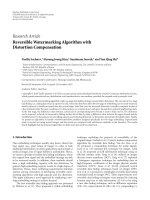
Figure 7: Effectiveness of repetition coding and error correction.
(a) Decoding BER before error correction. (b) Wordwise decoding

error rate using the block-repeating strategy and Hamming error
correction. BERs listed here are as obtained before repetition coding
and error correction.
instance, {1000011 } becomes {1000011 1000011
1000011
} if r = 3. For the second strategy to work, the
encoder has to know the length of music in advance, and the
hidden message should not be retrieved until the last rep-
etition block is decoded. Nevertheless, the block-repeating
strategy has an advantage. It is more effective in reducing the
BER if decoding errors tend to occur in adjacent bits. This is
clearly what we found empirically. In Figure 7, block repeti-
tion strategy (left panel, diamonds) consistently performed
better than bit repetition (dots). Results from different files
arecolor-coded,withblue
= clip 11, ch1; green = clip 12,
ch2; orange
= clip 14, ch1; red = clip 17, ch1.
In Figure 7, every data point is an average of 10 attempts
using randomized hidden message. Empirically, when the
raw BER
≤0.25, the block repetition strategy was able to re-
duce the error rate to <4% at r
= 13, which led to zero error
after Hamming correction. At a raw BER
= 0.33, however,
this coding scheme produced 8 word errors out of 90 trials.
With r
= 13, the data payload is (20 sec) × (43 bps)/13 ×
4/7 = 36 bits. In the future, if BER can be confined to <25%

under common signal processing procedures, F-QIM should
be useful for nonsecure applications. For applications with
more stringent security requirements, a private key would
need to be shared by the encoder and the decoder so the rep-
etition code is pseudorandomized.
10 EURASIP Journal on Information Security
4.3. Other suggestions for future research
To improve the performances against LPF, one can adopt a
multirate sinusoidal model [11] for watermark embedding.
At low frequency, a longer window can be used in D+S signal
decomposition to produce higher accuracy in frequency es-
timation. In this case, the data-hiding payload is reduced to
trade for enhanced robustness. At high frequency, the water-
mark encoding configuration can remain the same inasmuch
as to sustain HPF and high-quality AAC encoding.
7
The virtual room experiments (see Figure 5)canbere-
garded as a pilot study of robustness against the playback-
recording attack. The system currently shows an increase
in BER when the reflectivity of the virtual room increases
above R
= 0.6. Thus, the system is robust to echoes up to
R
= 0.6 in this room. It is promising that the increase in
BER is manageable in stereo-to-mono recording. However,
note that the distances between
{ch1, ch2} and the micro-
phone are carefully chosen to avoid desynchronization. The
delays are about 4.1 and 7.1 milliseconds from the two chan-
nels, or 180 samples and 312 samples (at F

s
= 44.1 kHz),
which are shorter than the window length h
= 512 at the
decoder.
To provide a mechanism of self-synchronization, in
the future, derived features from the trajectories could be
chosen as the watermark-embedding parameters. Higher-
dimensional quantization lattices, such as the spread trans-
form scalar Costa scheme [40]andvectorQIMcodes[41],
are worth of investigation. At the system level, an alterna-
tive approach is to embed another watermark in the transient
part to provide synchronization in time (e.g., [13, 15]). The
watermark carried by the deterministic components can thus
be recovered using synchronization information from the
transients’ watermark. This could be interesting for broad-
cast monitoring applications, and we foresee little conflict
in simultaneously embedding the two watermarks because
the sinusoidal and transient components are decoupled in
time.
In addition to watermarks embedded in tonal frequency
trajectories and transients, the “noise” component of a sines
+ noise + transients model might be utilized for watermark-
ing as well. To our knowledge, this has not been reported
previously although spread spectrum watermarking meth-
ods are obviously closely related. A “noise” watermark and
F-QIM watermark may mutually interfere since they over-
lap in both time and frequency. A noise-component water-
mark cannot be expected to survive perceptual audio coding
schemes as well as tonal and transient watermarks. However,

watermarks based on high-level features of the noise com-
ponent, such as overall bandwidth variations, power enve-
lope versus time, and other spectral feature variations over
time, should survive audio coding well enough, provided
that preservation of the chosen features is required for good
audio fidelity.
7
According to Apple Inc., “AAC compressed audio at 128 Kbps (stereo)
has been judged by expert listeners to be ‘indistinguishable’ from
the original uncompressed audio source.” (See />quicktime/technologies/aac/ for more information.)
Table 3:Listofconstantsandfrequentlyusedsymbols.
Symbol
Meaning
Default Value
F
s
Sampling rate
44.1 kHz
L
Blackman window length
2048
N
Hann window length
L/2
h
Hop size for sinusoidal
synthesis
N/2
N
FFT

FFT length after zero-padding
8 L at encoder;
8 h at decoder
i, j, k, m
Dummy indexes, with an ex-
ception that j can also refer
tothesquarerootof
−1 when
there is no confusion
—
n
Discrete time index
—
A
Linear amplitude
—
f
Frequency in Hz
—
ω
Frequency in rad/sample
—
φ
Phase
—
Δ f
Frequency quantization step
size
—
Finally, the listening test results suggest that there is still

room to diagnose the cause of artifacts, to modify the sig-
nal decomposing methods, and hence to improve the sound
qualities. It is very important for an audio watermarking
scheme to maximally preserve sound fidelity. To conclude,
audio watermarking through D+S signal decomposition is
still in its infancy, and many open ideas remain to be ex-
plored.
ACKNOWLEDGMENTS
The authors would like to thank the editors for encouraging
words and two anonymous reviewers for highly constructive
critiques. They also thank all friends who volunteered to take
the listening test and provided valuable feedback.
REFERENCES
[1] D. Kirovski and H. S. Malvar, “Spread-spectrum watermark-
ing of audio signals,” IEEE Transactions on Signal Processing,
vol. 51, no. 4, pp. 1020–1033, 2003.
[2] M. D. Swanson, B. Zhu, A. H. Tewfik, and L. Boney, “Robust
audio watermarking using perceptual masking,” Signal Pro-
cessing, vol. 66, no. 3, pp. 337–355, 1998.
[3] J. Chou, K. Ramchandran, and A. Ortega, “Next generation
techniques for robust and imperceptible audio data hiding,”
in Proceedings of IEEE International Conference on Acoustics,
Speech and Signal Processing (ICASSP ’01), vol. 3, pp. 1349–
1352, Salt Lake City, Utah, USA, May 2001.
[4] B. L. Vercoe, W. G. Gardner, and E. D. Scheirer, “Structured
audio: creation, transmission, and rendering of parametric
sound representations,” Proceedings of the IEEE, vol. 86, no. 5,
pp. 922–939, 1998.
[5] Y W. Liu and J. O. Smith, “Watermarking parametric repre-
sentations for synthetic audio,” in Proceedings IEEE Interna-

Y W.LiuandJ.O.Smith 11
tional Conference on Ac oustics, Speech and Signal Processing
(ICASSP ’03), vol. 5, pp. 660–663, Hong Kong, April 2003.
[6] J. D. Markel and A. H. Gray, Linear Prediction of Speech,
Springer, New York, NY, USA, 1976.
[7] M. R. Schroeder and B. S. Atal, “Code-excited linear prediction
(CELP): high-quality speech at very low bit rates,” in Proceed-
ings of IEEE International Conference on Acoustics, Speech and
Signal Processing (ICASSP ’85), vol. 10, pp. 937–940, Tampa,
Fla, USA, April 1985.
[8] R. J. McAulay and T. F. Quatieri, “Speech analysis/synthesis
based on a sinusoidal representation,” IEEE Transaction Acous-
tics, Speech, Signal Processing, vol. 34, no. 4, pp. 744–754, 1986.
[9] J.O.SmithandX.Serra,“PARSHL:ananalysis/synthesispro-
gram for non-harmonic sounds based on a sinusoidal repre-
sentation,” in Proceedings of the International Computer Music
Conference (ICMC ’87), pp. 290–297, Tokyo, Japan, 1987.
[10] X. Serra and J. O. Smith, “Spectral modeling synthesis: a
sound analysis/synthesis system based on a deterministic plus
stochastic decomposition,” Computer Music J ournal, vol. 14,
no. 4, pp. 12–24, 1990.
[11] S. N. Levine, “Audio representations for data compression and
compressed domain processing,” Ph.D. dissertation, Stanford
University, Stanford, Calif, USA, 1998.
[12] H. Purnhagen and N. Meine, “HILN-the MPEG-4 parametric
audio coding tools,” in Proceedings of the IEEE International
Symposium on Circuits and Systems (ISCAS ’00), vol. 3, pp.
201–204, Geneva, Switzerland, May 2000.
[13] C P. Wu, P C. Su, and C C. J. Kuo, “Robust and efficient dig-
ital audio watermarking using audio content analysis,” in Pro-

ceedings of Security and Watermarking of Multimedia Contents
II: Audio Watermarking, vol. 3971 of Proceedings of SPIE,pp.
382–392, San Jose, Calif, USA, January 2000.
[14] M. Ali, “Adaptive signal representation with application in au-
dio coding,” Ph.D. dissertation, University of Minnesota, Min-
neapolis, Minn, USA, 1996.
[15] M. F. Mansour and A. H. Tewfik, “Time-scale invariant audio
data embedding,” EURASIP Journal on Applied Signal Process-
ing, vol. 2003, no. 10, pp. 993–1000, 2003.
[16] W. Bender, D. Gruhl, N. Morimoto, and A. Lu, “Techniques for
data hiding,” IBM Systems Journal, vol. 35, no. 3-4, pp. 313–
336, 1996.
[17] X. Dong, M. F. Bocko, and Z. Ignjatovic, “Data hiding via
phase manipulation of audio signals,” in Proceedings IEEE In-
ternational Conference on Acoustics, Speech and Signal Process-
ing (ICASSP ’04), vol. 5, pp. 377–380, Montreal, QC, Canada,
May 2004.
[18] B. Chen and G. W. Wornell, “Quantization index modulation:
a class of provably good methods for digital watermarking
and information embedding,” IEEE Transactions on Informa-
tion Theory, vol. 47, no. 4, pp. 1423–1443, 2001.
[19] R. Petrovic, “Audio signal watermarking based on replica
modulation,” in Proceedings of the 5th International Conference
on Telecommunications in Modern Satellite, Cable and Broad-
casting Service (TELSIKS ’01), vol. 1, pp. 227–234, Nis, Yu-
goslavia, September 2001.
[20] S. Shin, O. Kim, J. Kim, and J. Choil, “A robust audio wa-
termarking algorithm using pitch scaling,” in Proceedings of
the 14th International Conference on Digital Signal Processing
(DSP ’02), pp. 701–704, Pine Mountain, GA, USA, October

2002.
[21] L. Girin and S. Marchand, “Watermarking of speech signals
using the sinusoidal model and frequency modulation of the
partials,” in Proceedings of IEEE International Conference on
Acoustics, Speech and Signal Processing (ICASSP ’04), vol. 1, pp.
633–636, Montreal, QC, Canada, May 2004.
[22] Y W. Liu and J. O. Smith, “Watermarking sinusoidal audio
representations by quantization index modulation in multi-
ple frequencies,” in Proceedings IEEE International Conference
on Acoustics, Speech and Signal Processing (ICASSP ’04), vol. 5,
pp. 373–376, Montreal, QC, Canada, May 2004.
[23] F. J. Harris, “On the use of windows for harmonic analysis
with the discrete Fourier transform,” Proceedings of the IEEE,
vol. 66, no. 1, pp. 51–83, 1978.
[24] M. Bosi, “Perceptual audio coding,” IEEE Signal Processing
Magazine, vol. 14, no. 5, pp. 43–49, 1997.
[25] E. Zwicker and H. Fastl, Psychoacoustics, Facts and Mo dels ,
Springer, Berlin, Germany, 1990.
[26] N. Jayant, J. Johnston, and R. Safranek, “Signal compression
basedonmodelsofhumanperception,”Proceedings of the
IEEE, vol. 81, no. 10, pp. 1385–1422, 1993.
[27] M. Bosi and R. E. Goldberg, Introduction to Digital Audio Cod-
ing and Standards, Kluwer Academic Publishers, Boston, Mass,
USA, 2003.
[28] I. J. Cox, M. L. Miller, and J. A. Bloom, Digital Watermarking,
Morgan Kaufmann, San Francisco, Calif, USA, 2002.
[29] E. Terhardt, “Calculating virtual pitch,” Hearing Research,
vol. 1, no. 2, pp. 155–182, 1979.
[30] M. Abe and J. O. Smith, “Design criteria for simple sinusoidal
parameter estimation based on quadratic interpolation of FFT

magnitude peaks,” in Proceedings of the 117th Audio Engineer-
ing Society Conventions and Conferences (AES ’04), p. 6256, San
Francisco, Calif, USA, October 2004.
[31] E. G. Shower and R. Biddulph, “Differential pitch sensitivity
of the ear,” Journal of the Acoustical Society of America, vol. 3,
no. 1A, pp. 275–287, 1931.
[32] C. C. Wier, W. Jesteadt, and D. M. Green, “Frequency discrim-
ination as a function of frequency and sensation level,” Journal
of the Acoustical Society of America, vol. 61, no. 1, pp. 178–184,
1977.
[33] F G.Zeng,Y Y.Kong,H.J.Michalewski,andA.Starr,“Per-
ceptual consequences of disrupted auditory nerve activity,”
Journal of Neurophysiology, vol. 93, no. 6, pp. 3050–3063, 2005.
[34] Y W. Liu, “Audio watermarking through parametric synthesis
models,” in Digital Audio Watermarking Techniques and Tech-
nologies: Applications and Benchmarking, N. Cvejic, Ed., Idea
Group, Hershey, Pa, USA, 2007.
[35] L. L. Scharf and L. T. McWhorter, “Geometry of the Cramer-
Rao bound,” in Proceedings of the 6th IEEE SP Workshop on
Statistical Signal and Array Processing, vol. 31, no. 3, pp. 301–
311, Victoria, BC, Canada, October 1992.
[36] M. Wolters, K. Kj
¨
orling, D. Homm, and H. Purnhagen, “A
closer look into MPEG-4 high efficiency AAC,” in Proceedings
of the 115th Audio Engineering Society Conventions and Confer-
ences (AES ’03), New York, NY, USA, October 2003.
[37] J. B. Allen and D. A. Berkley, “Image method for efficiently
simulating small-room acoustics,” Journal of the Acoustical So-
ciety of America, vol. 65, no. 4, pp. 943–950, 1979.

[38] P. Kabal, “An examination and interpretation of ITU-R
BS.1387: perceptual evaluation of audio quality,” Tech. Rep.,
Department of Electrical & Computer Engineering, McGill
University, Montreal, Canada, 2003.
.mcgill.ca/Documents/Software/.
[39] V. Pless, Introduction to the Theory of Error-Correcting Codes,
Wiley-Interscience, New York, NY, USA, 3rd edition, 1998.
12 EURASIP Journal on Information Security
[40] J. J. Eggers, R. B
¨
auml, R. Tzschoppe, and B. Girod, “Scalar
Costa scheme for information embedding,” IEEE Transactions
on Signal Processing, vol. 51, no. 4, pp. 1003–1019, 2003.
[41] P. Moulin and R. Koetter, “Data-hiding codes,” Proceedings of
the IEEE, vol. 93, no. 12, pp. 2083–2126, 2005.