Báo cáo hóa học: " Research Article Efficient Delay Tracking Methods with Sidelobes Cancellation for BOC-Modulated Signals" potx

Hindawi Publishing Corporation
EURASIP Journal on Wireless Communications and Networking
Volume 2007, Article ID 72626, 20 pages
doi:10.1155/2007/72626
Research Article
Efficient Delay Tracking Methods with Sidelobes
Cancellation for BOC-Modulated Signals
Adina Burian, Elena Simona Lohan, and Markku Kalevi Renfors
Institute of Communications Engineering, Tampere University of Technology, P.O. Box 553, 33101 Tampere, Finland
Received 26 September 2006; Accepted 2 July 2007
Recommended by Anton Donner
In positioning applications, where the line of sight (LOS) is needed with high accuracy, the accurate delay estimation is an im-
portant task. The new satellite-based positioning systems, such as Galileo and modernized GPS, will use a new modulation type,
that is, the binary offset carrier (BOC) modulation. This type of modulation creates multiple peaks (ambiguities) in the envelope
of the correlation function, and thus triggers new challenges in the delay-frequency acquisition and tracking stages. Moreover, the
properties of BOC-modulated signals are yet not well studied in the context of fading multipath channels. In this paper, sidelobe
cancellation techniques are applied with various tracking structures in order to remove or diminish the side peaks, while keep-
ing a sharp and narrow main lobe, thus allowing a better tracking. Five sidelobe cancellation methods (SCM) are proposed and
studied: SCM with interference cancellation (IC), SCM with narrow correlator, SCM with high-resolution correlator (HRC), SCM
with differential correlation (DC), and SCM with threshold. Compared to other delay tracking methods, the proposed SCM ap-
proaches have the advantage that they can be applied to any sine or cosine BOC-modulated signal. We analyze the performances of
various tracking techniques in the presence of fading multipath channels and we compare them with other methods existing in the
literature. The SCM approaches bring improvement also in scenarios with closely-spaced paths, which are the most problematic
from the accurate positioning point of view.
Copyright © 2007 Adina Burian et al. This is an open access article distributed under the Creative Commons Attribution License,
which permits unrestricted use, distribution, and reproduction in any medium, provided the original work is properly cited.
1. INTRODUCTION
Applications of new generations of Global Navigation Satel-
lite Systems (GNSS) are developing rapidly and attract a
great interest. The modernized GPS proposals have been re-
cently defined [1, 2] and the first version of Galileo (the

new European Satellite System) standards has been released
in May 2006 [3]. Both GPS and Galileo signals use direct
sequence-code division multiple access (DS-CDMA) tech-
nology, where code and frequency synchronizations are im-
portant stages at the receiver. The GNSS receivers estimate
jointly the code phase and the Doppler spreads through a
two-dimensional searching process in time-frequency plane.
This delay-Doppler estimation process is done in two phases,
first a coarse estimation stage (acquisition), followed by the
fine estimation stage (tracking). The mobile wireless chan-
nels suffer adverse effects during transmission, such as pres-
ence of multipath propagation, high level of noise, or ob-
struction of LOS by one or several closely spaced non-LOS
components (especially in indoor environments). The fading
of channel paths induces a certain Doppler spread, related
to the terminal speed. Also, the satellite movement induces
a Doppler shift, which deteriorates the performance, if not
correctly estimated and removed [4].
Since both the GPS and Galileo systems will send several
signals on the same carriers, a new modulation type has been
selected. This binary offset carrier (BOC) modulation has
been proposed in [5], in order to get a more efficient shar-
ing of the L-band spectrum by multiple civilian and military
users. The spectral efficiency is obtained by moving the signal
energy away from the band center, thus achieving a higher
degree of spectral separation between the BOC-modulated
signals and other signals which use the shift-keying mod-
ulation, such as the GPS C/A code. The BOC performance
has been studied for the GPS military M-signal [6] and later
has been also selected for the use with the new Galileo sig-

nals [3] and modernized GPS signals. The BOC modulation
is a square-wave modulation scheme, which uses the typi-
cal non-return-to-zero (NRZ) format [7]. While this type of
modulation provides better resistance to multipath and nar-
rowband interference [6], it triggers new challenges in the de-
lay estimation process, since deep fades (ambiguities) appear
2 EURASIP Journal on Wireless Communications and Networking
into the range of the ±1 chips around the maximum peak
of the correlation envelope. Since the receiver can lock on
a sidelobe peak, the tracking process has to cope with these
false lock points. In conclusion, the acquisition and track-
ing processes should counteract all these effects, and different
methods have been proposed in literature, in order to allevi-
ate multipath propagation and/or side-peaks ambiguities.
In order to minimize the influence of multipath errors,
which are the dominating error sources for many GNSS ap-
plications, several receiver-internal correlation approaches
have been proposed. During the 1990’s, a variety of receiver
architectures were introduced in order to mitigate the multi-
path for GPS C/A code or GLONASS. The traditional GPS re-
ceiver employs a delay-lock loop (DLL) with a spacing Δ be-
tween the early and late correlators of one chip. However, due
to presence of multipath, this wide DLL, which should track
the incoming signal within the receiver, is not able to align
perfectly the local code with the incoming signal, since the
presence of multipath (within a delay of 1.5 chips) creates a
bias of the zero-crossing point of the S-curve function. A first
approach to reduce the influences of code multipath is the
narrow correlator or narrow early minus-late (NEML) track-
ing loop introduced for GPS receivers by NovAtel [8]. Instead

of using a standard (wide) correlator, the chip spacing of a
narrow correlator is less than one chip (typically Δ
= 0.1
chips). The lower bound on the correlator spacing depends
on the available bandwidth. Correlator spacings of Δ
= 0.1
and Δ
= 0.05 chips are commercially available for GPS.
Another family of tracking loops proposed for GPS are
the so-called double-delta (ΔΔ) correlators, which are the
general name for special code discriminators which are
formed by two correlator pairs instead of one [9]. Some
well-known implementations of ΔΔ concept are the high-
resolution correlator (HRC) [10], the Ashtech’s Strobe Cor-
relator [11], or the NovAtel’s Pulse Aperture Correlator [12].
Another similar tracking method with ΔΔ structure is the
Early1/Early2 tracking [13],wheretwocorrelatorsarelo-
cated on the early slope of the correlation function (with
an arbitrary spacing); their amplitudes are compared with
the amplitudes of an ideal reference correlation function and
based on the measured amplitudes and reference amplitudes,
a delay correction factor is calculated. The Early1/Early2
tracker shows the worst multipath performance for short-
and medium-delay multipath compared to the HRC or the
Strobe Correlator [9].
The early late slope technique [9], also called Multipath
Elimination Technology, is based on determining the slope
at both sides of autocorrelation function’s central peak. Once
both slopes are known, they can be used to perform a pseu-
dorange correction. Simulation results showed that in multi-

path environments, the early late slope technique is outper-
formed by HRC and Strobe correlators [9]. Also, it should
be mentioned that in cases of Narrow Correlator, ΔΔ,early-
late slope, or Early1/Early2 methods the BOC(n,n)modu-
lated signal outperforms the BPSK modulated signals, for
multipath delays greater than approximately 0.5 chips (long-
delay multipath) [9]. A scheme based on the slope differen-
tial of the correlation function has been proposed in [14].
This scheme employs only the prompt correlator and in pres-
ence of multipath, it has an unbiased tracking error, unlike
the narrow or strobe correlators schemes, which have a bi-
ased tracking error due to the nonsymmetric property of the
correlation output. However, the performance measure was
solely based on the multipath error envelope curves, thus its
potential in more realistic multipath environments is still an
open issue. One algorithm proposed to diminish the effect
of multipath for GPS application is the multipath estimating
delay locked loop (MEDLL) [15]. This method is different in
that it is not based on a discriminator function, but instead
forms estimates of delay and phase of direct LOS signal com-
ponent and of the indirect multipath components. It uses
a reference correlation function in order to determine the
best combinations of LOS and NLOS components (i.e., am-
plitudes, delays, phases, and number of multipaths) which
would have produced the measured correlation function.
As mentioned above, in the case of BOC-modulated sig-
nals, besides the multipath propagation problem, the side-
lobes peaks ambiguities should be also taken into account. In
order to counteract this issue, different approaches have been
introduced. One method considered in [16] is the partial

Sideband discriminator, which uses weighted combinations
of the upper and lower sidebands of received signal, to obtain
modified upper and lower signals. A “bump-jumping” algo-
rithm is presented in [17]. The “bump-jumping” discrimi-
nator tracks the ambiguous offset that arises due to multi-
peaked Autocorrelation Function (ACF), making amplitude
comparisons of the prompt peak with those of neighbor-
ing peaks, but it does not resolve continuously the ambigu-
ity issue. An alternative method of preventing incorrect code
tracking is proposed in [18]. This technique relies on sum-
mation of two different discriminator S-curves (named here
restoring forces), derived from coherent, respectively non-
coherent combining of the sidebands. One drawback is that
there is a noise penalty which increases as carrier-to-noise
ratio (CNR) decreases, but it does not seem excessive [18]. A
new approach which design a new replica code and produces
a continuously unambiguous BOC correlation is described
in [19].
The methods proposed in [16–19] tend to destroy the
sharp peak of the ACF, while removing its ambiguities. How-
ever, for accurate delay tracking, preserving a sharp peak of
the ACF is a prerequisite. An innovative unambiguous track-
ing technique, that keeps the sharp correlation of the main
peak, is proposed in [20]. This approach uses two correlation
channels, completely removing the side peaks from the corre-
lation function. However, this method is verified for the par-
ticular case of SinBOC(n, n) modulated signals, and its ex-
tension to other sine or cosine BOC signals is not straightfor-
ward. A similar method, with a better multipath resistance, is
introduced in [21].

Another approach which produces a decrease of sidelobes
from ACF is the differential correlation method, where the
correlation is performed between two consecutive outputs of
coherent integration [22].
In this paper, we analyze in details and develop further a
novel class of tracking algorithms, introduced by authors in
Adina Burian et al. 3
[23]. These techniques are named the sidelobes cancellation
methods (SCM), because they are all based on the idea of
suppressing the undesired lobes of the BOC correlation en-
velope and they cope better with the false lock points (ambi-
guities) which appear due to BOC modulation, while keeping
the sharp shape of the main peak. It can be applied in both
acquisition and tracking stages, but due to narrow width of
the main peak, only the tracking stage is considered here.
In contrast with the approach from [20] (valid only for sine
BOC(n,n) cases), our methods have the advantage that they
can be generalized to any sine and cosine BOC(m, n)modu-
lation and that they have reduced complexity, since they are
based on an ideal reference correlation function, stored at re-
ceiver side. In order to deal with both sidelobes ambiguities
and multipath problems, we used the sidelobes cancellation
idea in conjunction with different discriminators, based on
the unambiguous shape of ACF (i.e., the narrow correlator,
the high resolution correlator), or after applying the differ-
ential correlation method. We also introduced here an SCM
method with multipath interference cancellation (SCM IC),
where the SCM is used in combination with a MEDLL unit,
and also an SCM algorithm based on threshold comparison.
This paper is organized as follows: Section 2 describes the

signal model in the presence of BOC modulation. Section 3
presents several representative delay tracking algorithms,
employed for comparison with the SCM methods. Section 4
introduces the SCM ideas and presents the SCM usage in
conjunction with other delay tracking algorithms or based
solely on threshold comparison. The performance evalua-
tion of the new methods with the existing delay estimators,
in terms of root mean square error (RMSE) and mean time
to lose lock (MTLL), is done in Section 5. The conclusions
are drawn in Section 6.
2. SIGNAL MODEL IN PRESENCE OF
BOC MODULATION
At the transmitter, the data sequence is first spread and the
pseudorandom (PRN) sequence is further BOC-modulated.
The BOC modulation is a square subcarrier modulation,
where the PRN signal is multiplied by a rectangular sub-
carrier which has a frequency multiple of code frequency. A
BOC-modulated signal (sine or cosine) creates a split spec-
trum with the two main lobes shifted symmetrically from the
carrier frequency by a value of the subcarrier frequency f
sc
[5].
The usual notation for BOC modulation is BOC( f
sc
, f
c
),
where f
c
is the chip frequency. For Galileo signals, the

BOC(m,n) notation is also used [5], where the sine and co-
sine BOC modulations are defined via two parameters m and
n, satisfying the relationships m
= f
sc
/f
ref
and n = f
c
/f
ref
,
where f
ref
= 1.023 MHz is the reference frequency [5, 24].
From the point of view of equivalent baseband signal, BOC
modulation can be defined via a single parameter, denoted
by the BOC-modulation order N
BOC
1
= 2m/n = 2 f
sc
/f
c
.The
factor N
BOC
1
is an integer number [25].
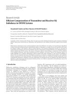
Examples of sine BOC-modulated waveforms for Sin-

BOC(1, 1) (even BOC-modulation order N
BOC
1
= 2) and
1
0
−1
012345
PRN sequence (N
BOC
1
= 1)
BOC-modulated
code
Chips
1
0
−1
012345
N
BOC
1
= 2
BOC-modulated
code
Chips
1
0
−1
012345

N
BOC
1
= 3
BOC-modulated
code
Chips
Figure 1: Examples of time-domain waveforms for sine BOC-
modulated signals.
SinBOC(15, 10) (odd BOC-modulation order N
BOC
1
= 3)
together with the original PRN sequence (N
BOC
1
= 1) are
shown in Figure 1. In order to consider the cosine BOC-
modulation case, a second BOC-modulation order N
BOC
2
=
2hasbeendefinedin[25], in a way that the case of sine BOC-
modulation corresponds to N
BOC
2
= 1 and the case of cosine
BOC modulation corresponds to N
BOC
2

= 2 (see the expres-
sions of (1)to(4)). After spreading and BOC modulation,
the data sequence is oversampled with an oversampled factor
of N
s
, and this oversampling determines the desired accuracy
in the delay estimation process. Thus, the oversampling fac-
tor N
s
represents the number of samples per BOC interval,
and one chip will consists of N
BOC
1
N
BOC
2
N
s
samples (i.e, the
chip period is T
c
= N
s
N
BOC
1
N
BOC
2
T

s
,whereT
s
is the sam-
pling rate).
The BOC-modulated signal s
n,BOC
(t) can be written, in
its most general form, as a convolution between a PRN se-
quence s
PRN
(t)andaBOCwaveforms
BOC
(t)[25]:
s
n,BOC
(t)
=
+∞

n=−∞
b
n
S
F

k=1
(−1)
nN
BOC

1
c
k,n
s
BOC

t − nT −kT
c

=
s
BOC
(t) ⊗
+∞

n=−∞
S
F

k=1
b
n
c
k,n
(−1)
nN
BOC
1
δ


t − nT −kT
c

=
s
BOC
(t) ⊗s
PRN
(t),
(1)
4 EURASIP Journal on Wireless Communications and Networking
where b
n
is the nth complex data symbol, T is the symbol
period (or code epoch length) (T
= S
F
T
c
), c
k,n
is the kth
chip corresponding to the nth symbol, T
c
= 1/f
c
is the chip
period, S
F
is the spreading factor (i.e., for GPS C/A signal

and Galileo OS signal, S
F
= 1023), δ(t) is the Dirac pulse,
⊗ is the convolution operator and s
PRN
(t) is the pseudo-
random (PRN) code sequence (including data modulation)
of satellite of interest, and s
BOC
(·) is the BOC-modulated
signal (sine or cosine) whose expression is given in (2)to
(4). We remark that the term (
−1)
nN
BOC
1
is included to take
into account also odd BOC-modulation orders, similar with
[26]. The interference of other satellites is modeled as addi-
tive white Gaussian noise, and, for clarity of notations, the
continuous-time model is employed here. However, the ex-
tension to the discrete-time model is straightforward and all
presented results are based on discrete-time implementation.
The SinBOC-CosBOC-modulated waveforms s
BOC
(t)are
defined as in [5, 25]:
s
sin / CosBOC
(t) =

⎧
⎪
⎪
⎪
⎨
⎪
⎪
⎪
⎩
sign

sin

N
BOC
1
πt
T
c

for SinBOC,
sign

cos

N
BOC
1
πt
T

c

for CosBOC,
(2)
respectively, that is, for SinBOC-modulation [25],
s
SinBOC
(t) =
N
BOC
1
−1

i=0
(−1)
i
p
T
B
1

t − i
T
c
N
BOC

,(3)
and for CosBOC-modulation [25],
s

CosBOC
(t) =
N
BOC
1
−1

i=0
N
BOC
2
−1

k=0
(−1)
i+k
× p
T
B

t − i
T
c
N
BOC
1
−k
T
c
N

BOC
1
N
BOC
2

.
(4)
In (3)and(4), p
T
B
1
(·) is a rectangular pulse of sup-
port T
c
/N
BOC
1
and p
T
B
(·) is a rectangular pulse of support
T
c
/N
BOC
1
N
BOC
2

.Forexample,
p
T
B
(t) =
⎧
⎪
⎨
⎪
⎩
1if0≤ t<
T
c
N
BOC
1
N
BOC
2
,
0 otherwise.
(5)
We remark that the bandlimiting case can also be taken into
account, by setting p
T
B
(·) to be equal to the pulse shaping
filter.
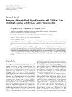
Some examples of the normalized power spectral den-
sity (PSD), computed as in [25], for several sine and cosine

BOC-modulated signals, are shown in Figure 2.Itcanbeob-
served that for even-modulation orders such as SinBOC(1, 1)
or CosBOC(10, 5) (currently selected or proposed by Galileo
Signal Task Force), the spectrum is symmetrically split into
two parts, thus moving the signal energy away from DC fre-
quency and thus allowing for less interference with the exist-
ing GPS bands (i.e., the BPSK case). Also, it should be men-
tioned that in case of an odd BOC-modulation order (i.e.,
−2 −1012
−120
−100
−80
−60
−40
−20
0
Frequency (MHz)
BPSK
SinBOC (1, 1)
SinBOC (15, 10)
CosBOC (10, 5)
Examples of PSD for different BOC-modulated signals
PSD (dB/Hz)
Figure 2: Examples of baseband PSD for BOC-modulated signals.
SinBOC(15, 10)), the interference around the DC frequency
is not completely suppressed.
The baseband model of the received signal r(t)viaafad-
ing channel can be written as [25]
r(t) =


E
b
e
+j2πf
D
t
n
=+∞

n=−∞
b
n
L

l=1
α
n,l
(t)
×s
n,sin / CosBOC

t − τ
l

+ η(t),
(6)
where E
b
is the bit or symbol energy of signal (one symbol is
equivalent with a code epoch and typically has a duration of

T
= 1 ms), f
D
is the Doppler shift introduced by channel, L
is the number of channel paths, α
n,l
is the time-varying com-
plex fading coefficient of the lth path during the nth code
epoch, τ
l
is the corresponding path delay (assuming to be
constant or slowly varying during the observation interval)
and η(
·) is the additive noise component which incorporates
the additive white noise from the channel and the interfer-
ence due to other satellites.
At the receiver, the code-Doppler acquisition and track-
ing of the received signal (i.e., estimating the Doppler shift f
D
and the channel delay τ
l
) are based on the correlation with a
reference signal s
ref
(t−τ,

f
D
, n
1

), including the PRN code and
the BOC modulation (here, n
1
is the considered symbol in-
dex):
s
ref

t − τ,

f
D
, n
1

=
e
−j2π

f
D
t
S
F

k=−1
c
k,n
1
N

BOC
1
−1

i=0
N
BOC
2
−1

j=0
(−1)
i+j
p
T
B

t − n
1
T − kT
c
−i
T
c
N
BOC
1
− j
T
c

N
BOC
1
N
BOC
2
− τ

.
(7)
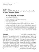
Some examples of the absolute value of the ideal ACF for
several BOC-modulated PRN sequences, together with the
Adina Burian et al. 5
BPSK case, are illustrated in Figure 3.Asitcanbeobserved,
for any BOC-modulated signal, there are ambiguities within
the
±1 chips interval around the maximum peak.
After correlation, the signal is coherently averaged over
N
c
ms, with the maximum coherence integration length dic-
tated by the coherence time of the channel, by possible resid-
ual Doppler shift errors and by the stability of oscillators. If
the coherent integration time is higher than the coherence
time of the channel, the spectrum of the received signal will
be severely distorted. The Doppler shift due to satellite move-
ment is estimated and removed before performing the coher-
ent integration. For further noise reduction, the signal can be
noncoherently averaged over N
nc

blocks; however there are
some squaring losses in the signal power due to noncoher-
ent averaging. The delay estimation is performed on a code-
Doppler search space, whose values are averaged correlation
functions with different time and frequency lags, with max-
ima occurring at f
= f
D
and τ = τ
l
.
3. EXISTING DELAY ESTIMATION ALGORITHMS IN
MULTIPATH CHANNELS
The presence of multipath is an important source of error
for GPS and Galileo applications. As mentioned before, tra-
ditionally, the multipath delay estimation block is imple-
mented via a feedback loop. These tracking loop methods are
based on the assumption that a coarse delay estimate is avail-
able at receiver, as result of the acquisition stage. The tracking
loop is refining this estimate by keeping the track of the pre-
vious estimate.
3.1. Narrow early minus late (NEML) correlator
One of the first approaches to reduce the influences of code
multipath is the narrow early minus late correlation method,
first proposed in 1992 for GPS receivers [8]. Instead of us-
ing a standard correlator with an early late spacing Δ of 1
chip, a smaller spacing (typically Δ
= 0.1 chips) is used.
Two correlations are performed between the incoming sig-
nal r(t) and a late (resp., early) version of the reference code

s
ref
Early,Late
(t − τ ± Δ/2), where s
ref
Early,Late
(·) is the advanced or
delayed BOC-modulated PRN code and
τ is the tentative
delay estimate. The early (resp., late) branch correlations
R
early,Late
(·)canbewrittenas
R
Early,Late
(τ) =

N
c
r(t)s
ref
Early,Late

t − τ ±
Δ
2

dt. (8)
These two correlators spaced at Δ (e.g., Δ
= 0.1 chips) are

used in the receiver in order to form the discriminator func-
tion. If channel and data estimates are available, the NEML
loops are coherent. Typically, due to low CNR and residual
Doppler errors from GPS and Galileo systems, noncoherent
NEML loops are employed, when squaring or absolute value
are used in order to compensate for data modulation and
channelvariations.TheperformanceofNEMLisbestillus-
trated by the S-curve, which presents the expected value of
error as a function of code phase error. For NEML, the two
1
0.9
0.8
0.7
0.6
0.5
0.4
0.3
0.2
0.1
0
−1.5 −1 −0.500.511.5
Normalized ACFs
Chips
Ideal ACF for BOC-modulated signals
BPSK
SinBOC (1, 1)
SinBOC (15, 10)
CosBOC (10, 5)
Figure 3: Examples of absolute value of the ACF for BOC-
modulated signals.

branches are combined noncoherently, and the S-curve is ob-
tained as in (9),
S
NEML
(τ) =


R
Late
(τ)


2
−|R
Early
(τ)


2
. (9)
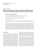
The error signal given by the S-curve is fed back into
a loop filter and then into a numeric controlled oscilla-
tor (NCO) which advances or delays the timing of the ref-
erence signal generator. Figure 4 illustrates the S-curve in
single path channel, for BPSK, SinBOC(1, 1), respectively,
SinBOC(10, 5) modulated signals. The zerocrossing shows
the presence of channel path, that is, the zero delay er-
ror corresponds to zero feedback error. However, for BOC-
modulated signals, due to sidelobes ambiguities, the early late
spacing should be less than the width of the main lobe of

the ACF envelope, in order to avoid the false locks. Typically,
for BOC(m, n) modulation, this translates to approximately
Δ
≤ n/4m.
3.2. High-resolution correlator (HRC)
The high-resolution correlator (HRC), introduced in [10],
can be obtained using multiple correlator outputs from con-
ventional receiver hardware. There are a variety of combi-
nations of multiple correlators which can be used to imple-
ment the HRC concept, which yield similar performance.
The HRC provides significant code multipath mitigation for
medium and long delay multipath, compared to the con-
ventional NEML detector, with minor or negligible degrada-
tion in noise performance. It also provides substantial carrier
phase multipath mitigation, at the cost of significantly de-
graded noise performance, but, it does not provide rejection
of short delay multipath [10]. The block diagram of a non-
coherent HRC is shown in Figure 5. In contrast to the NEML
structure, two new branches are introduced, namely, a very
6 EURASIP Journal on Wireless Communications and Networking
1
0.8
0.6
0.4
0.2
0
−0.2
−0.4
−0.6
−0.8

−1
−1.5 −1 −0.500.511.5
Normalized S-curve
Delay error (chips)
Ideal S-curve (no multipath) for
BOC-modulated and BPSK signals
BPSK
SinBOC (1, 1)
SinBOC (10, 5)
Figure 4: Ideal S-curves for BOC-modulated and BPSK signals
(NEML, Δ
= 0.1 chips).
I & D on
N
c
msec
I & D on
N
c
msec
I & D on
N
c
msec
I & D on
N
c
msec
Late code
Early code

Ve r y e a r l y c o d e
Ve r y l a t e c o d e
Constant factor a
NCO
Loop filter
r(t)
+
−
+
+
+
−
||
2
||
2
||
2
||
2
Figure 5: Block diagram for HRC tracking loop.
early and, respectively, a very late branch. The S-curve for a
noncoherent five-correlator HRC can be written as in [10]:
S
HRC
(τ) =


R
Late

(τ)


2
−


R
Early
(τ)


2
+ a



R
Ve r y L a t e
(τ)


2
−


R
Ve r y E a r l y
(τ)



2

,
(10)
where R
Ve r y L a t e
(·)andR
Ve r y E a r l y
(·) are the very late and very
early correlations, with the spacing between them of 2Δ
chips, and a is a weighting factor which is typically
−1/2[10].
Examples of S-curves for HRC in the presence of a sin-
gle path static channel, are shown in Figure 6, for two BOC-
modulated signals. The early late spacing is Δ
= 0.1 chips
(i.e., narrow correlator), thus the main lobes around zero
crossing are narrower, and it is more likely that the separa-
tion between multiple paths will be done more easily.
1
0.8
0.6
0.4
0.2
0
−0.2
−0.4
−0.6
−0.8

−1
−1.5 −1 −0.50 0.511.5
Normalized S-curve
Delay error (chips)
Ideal S-curve (no multipath) for two BOC-modulated signals
SinBOC (1, 1)
SinBOC (10, 5)
Figure 6: Ideal S-curves for noncoherent HRC with a =−1/2, for
two BOC-modulated signals and Δ
= 0.1 chips.
3.3. Multipath estimating delay locked loop (MEDLL)
Adifferent approach, proposed to remove the multipath ef-
fects for GPS C/A delay tracking is the multipath estima-
tion delay locked l;oop [15]. The MEDLL method estimates
jointly the delays, phases, and amplitudes of all multipaths,
canceling the multipath interference. Since it is not based on
an S-curve, it can work in both feedback and feedforward
configurations. To the authors’ knowledge, the performance
of MEDLL algorithm for BOC modulated signals is still not
well understood, therefore, would be interesting to study a
similar approach. The steps of the MEDLL algorithm (as im-
plemented by us) are summarized bellow.
(i) Calculate the correlation function R
n
(t) for the nth
transmitted code epoch. Find out the maximum peak
of the correlation function and the corresponding de-
lay
τ
1

,amplitudea
1,n
,andphase

θ
1,n
.
(ii) Subtract the contribution of the calculated peak, in or-
der to have a new approximation of the correlation
function R
(1)
n
(τ) = R
n
(τ) − a
1,n
R
ref
(t − τ
1,n
)e
j

θ
1,n
.Here
R
ref
(·) is the reference correlation function, in the ab-
sence of multipaths (which can be, for example, stored

at the receiver). Find out the new peak of the residual
function R
(1)
n
(·) and its corresponding delay τ
2,n
,am-
plitude
a
2,n
,andphase

θ
2,n
. Subtract the contribution
of the new peak of residual function from R
(1)
n
(t)and
find a new estimate of the first peak. For more than
two peaks, the procedure is continued until all desired
peaks are estimated.
(iii) The previous step is repeated until a certain criterion
of convergence is met, that is, when residual function
is below a threshold (e.g., set to 0.5here)oruntil
Adina Burian et al. 7
1
0.9
0.8
0.7

0.6
0.5
0.4
0.3
0.2
0.1
0
−1.5 −1 −0.500.511.5
Normalized ACF
Delay error (chips)
Ideal ACFs (no multipath) for SinBOC (1, 1)-modulated signal
Non-coherent integration
Differential correlation
Figure 7: Envelope correlation function of traditional noncoher-
ent integration and differential correlation for a SinBOC(1, 1)-
modulated signal.
the moment when introducing a new delay does not
improve the performance in the sense of root mean
square error between the original correlation function
and the estimated correlation function.
3.4. Differential correlation (DC)
Originally proposed for CDMA-based wireless communi-
cation systems, the differential correlation method has also
been investigated in context of GPS navigation system [22]. It
has been observed that with low and medium coherent times
of the fading channel and in absence of any frequency error,
this approach provides better resistance to noise than the tra-
ditional noncoherent integration methods. In DC method,
the correlation is performed between two consecutive out-
puts of coherent integration. These correlation variables are

then integrated, in order to obtain a differential variable. The
differential detection variable z is given as
z
DC
=
1
M −1
M−1

k=1


y
∗
k
y
k+1


2
, (11)
where y
k
, k = 1, , M are the outputs of the coherent in-
tegration and M is the differential integration length. For a
fair comparison between the differential noncoherent and
traditional noncoherent methods, here it is assumed that
M
= N
nc

,whereN
nc
is the noncoherent integration length.
Since the differential coherent correlation method was no-
ticed to be more sensitive to residual Doppler errors, only
the differential noncoherent correlation is considered here.
The analysis done in [22] is limited to BPSK modulation.
From Figure 7, it can be noticed that applying the DC to a
BOC-modulated signal, instead of the conventional nonco-
herent integration, the sidelobes envelope can be decreased,
and thus this method has a potential in reducing the side
peaks ambiguities.
3.5. Nonambiguous BOC(n, n) signal tracking
(Julien&al. method)
A recent tracking approach, which removes the sidelobes
ambiguities of SinBOC(n, n) signals and offers an improved
resistance to long-delay multipath, has been introduced in
[20]. This method, referred here as Julien&al. method,af-
ter the name of the first author in [20], has emerged while
observing the ACF of a SinBOC(1, 1) signal with sine phas-
ing, and the cross correlation of SinBOC(1, 1) signal with its
spreading sequence. The ideal correlation function R
ideal
BOC
(·)
for SinBOC(1, 1)-modulated signals in the absence of multi-
paths, can be written as [25]
R
ideal
BOC

(τ) = Λ
T
c
/2
(τ) −
1
2
Λ
T
c
/2

τ −
T
c
2

−
1
2
Λ
T
c
/2

τ +
T
c
2


,
(12)
where Λ
T
c
/2
(τ − α) is the value in τ of a triangular function
1
centered in α, with a width of 1-chip, T
c
is the chip period,
and τ is the code delay in chips.
The cross correlation of a SinBOC(1, 1) signal with the
spreading pseudorandom code, for an ideal case (no multi-
paths and ideal PRN code), can be expressed as [20]
R
ideal
BOC,PRN
(τ) =
1
2

Λ
T
c
/2

τ +
T
c

2

+ Λ
T
c
/2

τ −
T
c
2

.
(13)
Two types of DLL discriminators have been considered
in [20], namely, the early-minus- late- power (EMLP) dis-
criminator and the dot-product (DP) discriminator. These
examples of possible discriminators result from the use of
the combination of BOC-autocorrelation function and of
the BOC/PRN-correlation function [20]. Based on (12)and
(13), the ideal EMLP discriminator is constructed, as in (14),
where τ is the code tracking error [20]:
S
ideal
EMLP
(τ) =

R
ideal
2

BOC

τ +
Δ
2

−
R
ideal
2
BOC

τ −
Δ
2

−

R
ideal
2
BOC,PRN

τ +
Δ
2

−
R
ideal

2
BOC,PRN

τ −
Δ
2

.
(14)
The alternative DP discriminator variant [20]doesnot
have a linear variation as a function of code tracking error:
S
ideal
DP
(τ)
=

R
ideal
2
BOC

τ +
Δ
2

−
R
ideal
2

BOC

τ −
Δ
2

R
ideal
2
BOC
(τ)
−

R
ideal
2
BOC,PRN

τ +
Δ
2

−
R
ideal
2
BOC,PRN

τ −
Δ

2

R
ideal
2
BOC
(τ).
(15)
1
Our notation is equivalent with the notation tri
α
(x/y)usedin[20], via
tri
α
(τ/y) = Λ
T
c
/2
(τ − αT
c
/y).
8 EURASIP Journal on Wireless Communications and Networking
1
0.5
0
−1.5 −1 −0.500.511.5
SinBOC (1, 1) modulation, ACFs of
BOC-modulated and subtracted signals
Continue line:
BOC-modulated signal

Dashed line:
subtracted signal
Delay (chips)
1
0.5
0
−1.5 −1 −0.500.511.5
SinBOC (1, 1) modulation, ACF of unambiguous signal
Unambiguous signal
Delay (chips)
Figure 8: SinBOC(1, 1)-modulated signal: examples of the ambigu-
ous correlation function and subtracted pulse (upper plot) and
the obtained unambiguous correlation function (lower plot), for a
single-path channel.
Since the resulting discriminators remove the effect of
SinBOC(1, 1) modulation, there are no longer false lock
points, and the narrow structure of the main correlation lobe
is preserved [20]. Indeed, the side peaks of SinBOC(1, 1)
correlation function R
ideal
BOC
(τ) have the same magnitude
and same location as the two peaks of SinBOC(1, 1)/PRN-
correlation function R
ideal
BOC,PRN
(τ). By subtracting the squares
of the two functions, a new synthesized correlation function
is derived and the two side peaks of SinBOC(1,1) correlation
function are canceled almost totally, while still keeping the

sharpness of the main lobe (Figure 8). Two small negative
sidelobes appear next to the main peak (about
±0.35 chips
around the global maximum), but since they point down-
wards, they do not bring any threat [20]. The correlation val-
uesspacedatmorethan0.5 chips apart from the global peak
are very close to zero, which means a potentially strong resis-
tance to long-delay multipath.
In practice, the discriminators S
EMLP
(τ)orS
DP
(τ), as
givenin[20], are formed via continuous computation, at re-
ceiver side, of correlation functions R
BOC
(·)andR
BOC,PRN
(·)
values, not on the ideal ones. In practice, R
BOC
(·) is the
correlation between the incoming signal (in the presence of
multipaths) and the reference BOC-modulated code, and
R
BOC,PRN
(·) is the correlation between the incoming signal
and the pseudorandom code (without BOC modulation).
This method has been applied only to SinBOC(n, n) signals.
Moreover, instead of making use of the ideal reference func-

tion R
ideal
BOC,PRN
(·) (which can be computed only once and
stored at the receiver side), the correlation R
BOC,PRN
(·) needs
to be computed for each code epoch in [20]. Of course, in or-
der to make use of the R
ideal
BOC,PRN
(·) shape, we also need some
information about channel multipath profile. This will be ex-
plained in the next section.
4. SIDELOBES CANCELLATION METHOD (SCM)
In this section, we introduce unambiguous tracking ap-
proaches based on sidelobe cancellation; all these approaches
are grouped under the generic name of sidelobes cancel-
lation methods). The SCM technique removes or dimin-
ishes the threats brought by the sidelobes peaks of the
BOC-modulated signals. In contrast with the Julien&al.
method, which is restricted to the SinBOC(n, n)case,we
will show here how to use SCM with any sine or cosine
BOC-modulated signal. The SCM approach uses an ideal
reference correlation function at receiver, which resembles
the shapes of sidelobes, induced by BOC modulation. In
order to remove the sidelobes ambiguities, this ideal refer-
ence function is subtracted from the correlation of the re-
ceived BOC-modulated signal with the reference PRN code.
In the Julien&al. method, the subtraction function, which

approximates the sidelobes, is provided by cross-correlating
the spreading PRN code and the received signal. Here, this
subtraction function is derived theoretically, and computed
only once per BOC signal. Then, it is stored at the receiver
side in order to reduce the number of correlation operations.
Therefore, our methods provide a less time-consuming and
simpler approach, since the reference ideal correlation func-
tion is generated only once and can be stored at receiver.
4.1. Ideal reference functions for SCM method
In this subsection, we explain how the subtraction pulses
are computed and then applied to cancel the undesired side-
lobes.
Following derivations similar with those from [25]and
intuitive deductions, we have derived the following ideal ref-
erence function to be subtracted from the received signal af-
ter the code correlation:
R
ideal
sub
(τ) =
N
BOC
1
−1

i=0
N
BOC
1
−1


j=0
N
BOC
2
−1

k=0
N
BOC
2
−1

l=0
(−1)
i×j+k+l
Λ
T
B

τ +(i − j)T
B
+(k − l)
T
B
N
BOC
2

,

(16)
where T
B
= T
c
/N
BOC
1
N
BOC
2
is the BOC interval, Λ
T
B
(·)
is the triangular function centered at 0 and with a width
of 2T
B
-chips, N
BOC
1
is the sine BOC-modulation order
(e.g., N
BOC
1
= 2 for SinBOC(1, 1), or N
BOC
1
= 4
for SinBOC(10, 5)) [25], and N

BOC
2
is the second BOC-
modulation factor which covers sine and cosine cases, as ex-
plained in [25] (i.e., if sine BOC modulation is employed,
N
BOC
2
= 1 and, if cosine BOC modulation is employed,
N
BOC
2
= 2).
As an example, the simplest case of SinBOC(1, 1)-
modulation (i.e., the main choice for Open Services in
Galileo), (16)becomes
R
ideal
sub,SinBOC(1,1)
(τ) =

Λ
T
B

τ −T
B

+ Λ
T

B

τ + T
B

, (17)
Adina Burian et al. 9
which is similar with Julien& al. expression of (13) with the
exception of a 1/2 factor (here, T
B
= T
c
/2).
The Sin- and CosBOC(m, n)-based ideal autocorrelation
function can be written as [25]
R
ideal
BOC
(τ) =
N
BOC
1
−1

i=0
N
BOC
1
−1


j=0
N
BOC
2
−1

k=0
N
BOC
2
−1

l=0
(−1)
i+j+k+l
Λ
T
B

τ +(i − j)T
B
+(k − l)
T
B
N
BOC
2

.
(18)

Again, for SinBOC(1, 1) case, the expression of (18)reduces
to
R
ideal
SinBOC(1,1)
(τ)
=

2Λ
T
B
(τ) −Λ
T
B

τ −T
BOC

−Λ
T
B

τ + T
BOC

,
(19)
which is, again, similar to Julien& al. expression of (12)with
the exception of a 1/2 factor (for SinBOC(1, 1), T
BOC

= T
c
/2,
N
BOC
1
= 2andN
BOC
2
= 1).
We remark that the difference between (16)and(18)
stays in the power of
−1 factor, that is, (16) stands for an ap-
proximation of the sidelobe effects (no main lobe included),
while (18) is the overall ACF (including both the main lobe
and the side lobes). The next step consists in canceling the ef-
fect of sidelobes (16) from the overall correlation (18), after
normalizing them properly.
Thus, in order to obtain an unambiguous ACF shape, the
squared function (R
ideal
sin
(·))
2
,(R
ideal
cos
(·))
2
, respectively, has to

be subtracted from the ambiguous squared correlation func-
tion as shown in
R
ideal
unamb
(τ) =

R
ideal
BOC
(τ)

2
−w

R
ideal
sin / cos
(τ)

2
, (20)
where w<1 is a weight factor used to normalize the reference
function (to achieve a magnitude of 1).
For example, for SinBOC(1, 1) and w
= 1, we get from
(17), (19), and (20), after straightforward computations, that
R
ideal
unamb

(τ) = 4

Λ
2
T
B
(τ) −Λ
T
B
(τ)Λ
T
B

τ −T
BOC

−Λ
T
B
(τ)Λ
T
B

τ + T
BOC

,
(21)
andifweplotR
ideal

unamb
(τ) (e.g., see the lower plot of Figure 8),
we get a main narrow correlation peak, without sidelobes.
All the derivations so far were based on ideal assumptions
(ideal correlation codes, single path static channels, etc.).
However, in practice, we have to cope with the real signals,
so the ideal autocorrelation function R
ideal
BOC
(τ) should be re-
placed with the computed correlation R
BOC
(τ) between the
received signal and the reference BOC-modulated pseudo-
random code. Thus, (20)becomes
R
unamb
(τ) =

R
BOC
(τ)

2
−w

R
ideal
sin / cos
(τ)


2
. (22)
Here comes into equation the weighting factor, since vari-
ous channel effects (such as noise and multipath) can mod-
ify the levels of R
BOC
(τ) function. In order to perform the
1
0.5
0
−1.5 −1 −0.500.511.5
CosBOC (10, 5) modulation, ACFs of
BOC-modulated and subtracted signals
Continue line:
BOC-modulated signal
Dashed line:
subtracted signal
Delay (chips)
1
0.5
0
−1.5 −1 −0.500.511.5
CosBOC (10, 5) modulation, ACF of unambiguous signal
Unambiguous signal
Delay (chips)
Figure 9: CosBOC(10, 5)-modulated signal: examples of the am-
biguous correlation function and subtracted pulse (upper plot)
and obtained unambiguous correlation function (lower plot), in a
single-path channel.

normalization of reference function (i.e., to find the weight
factors w), the peaks magnitudes of R
BOC
(·)functionarefirst
found out and sorted in increased order. Then the weighting
factor w is computed as the ratio between the last-but-one
peak and the highest peak. We remark that the above algo-
rithm does not require the computation of the BOC/PRN
correlation anymore, it only requires the computation of
R
BOC
(τ) = R
n
(τ) correlation. The pulses to be subtracted are
always based on the ideal functions R
ideal
sin / cos
(τ), and therefore,
they can be computed only once (via (16)) and stored at the
receiver (in order to decrease the complexity of the tracking
unit).
By comparison with Julien&al. method, here the num-
ber of correlations at the receiver is reduced by half (i.e.,
R
BOC,PRN
(·) computation is not needed anymore). Thus the
SCM technique offers less computational burden (only one
correlation channel in contrast to Julien&al. method, which
uses two correlation channels).
Figures 8 and 9 show the shapes of the ideal ambigu-

ous correlation functions and of the subtracted pulses, to-
gether with the correlation functions, obtained after subtrac-
tion (SCM method). Figure 8 exemplifies a SinBOC(1, 1)-
modulated signal, while Figure 9 illustrates the shapes for a
CosBOC(10, 5)-modulation case. As it can be observed, for
both SinBOC and CosBOC modulations, the subtractions
removes the sidelobes closest to the main peak, which are
the main threats in the tracking process. Also, it should be
mentioned that the Figure 8,foraSinBOC(1,1)modulated
signal, is also illustrative for the Julien&al. method, since the
shapes of correlation functions are similar with those pre-
sented in [20].
Equation (20) is valid for single path channels. How-
ever, in multipath presence, delay errors due to multipaths
10 EURASIP Journal on Wireless Communications and Networking
are likely to appear. When (22) is applied in this situation,
one important issue is to align the subtraction pulse to the
LOS peak (otherwise, the subtraction of (22) will not can-
cel the correct sidelobes). This can be done only if some ini-
tial estimate of LOS delay is obtained. For this purpose, we
employ and compare several feedback loops or feedforward
algorithms, as it will be explained next.
4.2. SCM with interference cancellation (IC)
Combining the multipath eliminating DLL concept with the
SCM method, we obtain an improved SCM technique with
multipath interference cancellation (SCM w ith IC). In this
method, the initial estimate of LOS delay is obtained via
MEDLL algorithm. The sidelobe cancellation is applied in-
side the iterative steps of MEDLL, as explained below.
(1) Calculate the correlation function R

n
(τ) between the
received signal and the reference BOC-modulated
code (e.g., see the continuous line, Figure 10,up-
per plot). Find the global maximum peak (the peak
1) of this correlation function, max
τ
|R
n
(τ)|, and its
corresponding delay,
τ
1,n
,amplitudea
1,n
and phase

θ
1,n
(e.g., the peak situated at the 50th-sample delay,
Figure 10,upperplot).
(2) Compute the ideal reference function centered at
τ
1,n
:
R
ideal
sub
(τ − τ
1,n

)via(16) (see the dashed line, Figure 10,
upper plot).
(3) Build an initial estimate of the channel impulse re-
sponse (CIR) based on
τ
1,n
, a
1,n
,and

θ
1,n
(e.g., the es-
timated CIR of peak 1, Figure 10,upperplot).
(4) In order to remove the sidelobes ambiguities, the
function R
ideal
sub
(τ − τ
1,n
) is then subtracted from the
multipath correlation function R
n
(τ) and an unam-
biguous shape is obtained, using (22), or, equiva-
lently R
n,unamb
(τ) = (R
n
(τ))

2
− (R
ideal
sub
(τ − τ
1,n
))
2
.In
Figure 10, the unambiguous ACF R
n,unamb
(·) is plot-
ted with dashed-dotted line, in both upper and lower
plots.
(5) Cancel out the contribution of the strongest path
and obtain the residual function R
(1)
n,unamb
(τ) =
R
n,unamb
(τ) − a
1,n
R
ideal
unamb
(τ)(τ − τ
1,n
)e
j


θ
1,n
,where
R
ideal
unmab
(τ) is the unambiguous reference function
given by (20). The shape of residual function is
exemplified in Figure 10, lower plot (drawn with
continuous line).
(6) The new maximum peak of the residual function
R
(1)
n,unamb
is found out (e.g., at 44th-sample delay,
Figure 10, lower plot), with its corresponding de-
lay
τ
2,n
,amplitudea
2,n
and phase

θ
2,n
.Thecon-
tributions of both peaks 1 and 2 are subtracted
from unambiguous correlation function R
n,unamb

(τ)
1
0.8
0.6
0.4
0.2
0
0 1020304050607080
Samples
Exemplification of SCM IC method (steps 1 to 4)
Original ACF
Estimated CIR
Subtracted ideal function
Unambiguous ACF
1
0.8
0.6
0.4
0.2
−0.2
0
0 1020304050607080
Samples
Exemplification of SCM IC method (steps 5 to 6)
Unambiguous ACF
Residual function
Estimated CIR, 2nd peak
Figure 10: Exemplification of SCM IC method, 2-paths fading
channel with true channel delay at 44 and 50 samples, average path
powers [

−2, 0] dB, SinBOC(1,1)-modulated signal.
and the maximum global peak is re-estimated from
R
(2)
n,unamb
(τ) = (R
n,unamb
(τ))
2
− (a
1,n
R
ideal
unamb
(τ)(τ −

τ
1,n
)e
j

θ
1,n
+ a
2,n
R
ideal
unamb
(τ)(τ − τ
2,n

)e
j

θ
2,n
)
2
.
(7) The steps (3) to (6) are repeated until all desired peaks
are estimated and until the residual function is below
a threshold value. In the example of Figure 10,after6
stepsbothpathdelaysareestimatedcorrectly.
ThesestepsofSCMICmethodareillustratedin
Figure 10, for 2-path fading channel.
Adina Burian et al. 11
1
0.8
0.6
0.4
0.2
0
−0.2
−0.4
−0.6
−0.8
−1
−1.5 −1 −0.50 0.511.5
Normalized S-curve
Delay error (chips)
Ideal S-curve (no multipath), SCM NEML method

SinBOC (1, 1)
SinBOC (10, 5)
Figure 11: SCM NEML method: ideal S-curves (no multipath), for
two BOC-modulation cases and Δ
= 0.1 chips.
4.3. SCM using narrow early minus lat discriminator
(SCM NEML)
After obtaining an unambiguous correlation function
R
n,unamb
(τ) (as it was shown in the previous section, steps
(1) to (4)), a NEML S-curve is constructed, by forming the
early, respectively, late branches, spaced at Δ
= 0.1 chips. The
S-curve is obtained in the same way as in Section 3.1,bysub-
tracting the late and early branches of unambiguous correla-
tion function,
S
SCM
NEML
(τ) =


R
Late
n,unamb
(τ)


2

−


R
Early
n,unamb
(τ)


2
. (23)
Examples of S-curves obtained with this method, in
presence of a single path static channel, are presented in
Figure 11, for two BOC-modulated signals, SinBOC(1, 1)
and SinBOC(10,5), and a spacing of Δ
= 0.1 chips. Com-
paring with Figure 4, which presents the NEML S-curves for
ambiguous signals, in Figure 11, the possibility to detect an
incorrect zero crossing, due to sidelobes peaks, is decreased.
A typical measure of performance for the ability of a de-
lay tracking loop to deal with multipath error is the so-called
multipath error envelope (MEE) [9, 10]. The MEE is usu-
ally computed for one direct and one reflected channel paths,
with a certain variable spacing. The multipath errors are cal-
culated for the worst-case scenario, when the two paths are
added inphase (upper MEE) and have equal strength, and
also, when the two paths are out of phase (lower MEE). Com-
parisons of MEEs plots, for both NEML and SCM NEML
methods, are shown in Figure 12, for two BOC-modulated
signals. A static channel with two paths of equal amplitudes

and variable spacing was considered. The only interference
considered here is the multipath interference, and the addi-
tive white noise effect is not taken into account. As it can be
seen in Figure 12, comparing with the NEML correlator, the
10
0
−10
00.20.40.60.81
Multipath error
envelope (meters)
SinBOC (1, 1), Δ = 0.1 chips
Multipath spacing (chips)
NEML correlator
SCM NEML method
10
0
−10
00.20.40.60.81
Multipath error
envelope (meters)
SinBOC (10, 5), Δ = 0.1 chips
Multipath spacing (chips)
NEML correlator
SCM NEML method
Figure 12: Multipath error envelopes (in meters): NEML correlator
versus SCM NEML method, for two BOC-modulation cases and
Δ
= 0.1 chips.
SCM NEML method brings a decrease in the errors of mul-
tipath envelopes, for both SinBOC(1, 1) and SinBOC(10, 5)

signals. We remark that the variations of the lower delay er-
ror envelope in the lower plot of Figure 12 are due to, on one
hand, the errors in the zero-crossing estimation algorithm,
and, on the other hand, to the fact that worse MEE is not
necessarily guaranteed when the paths are out of phase for
the noncoherent NEML.
4.4. SCM using high-resolution correlator
discriminator (SCM HRC)
In a similar manner as in previous section, the SCM method
can be also used in conjunction with an HRC discrimina-
tor, after removing the side peaks threats and obtaining an
unambiguous correlation function R
n,unamb
(τ). Based on this
unambiguous function, an HRC S-curve is constructed, in an
analogous way as in Section 3.2:
S
SCM
HRC
(τ) =


R
Late
n,unamb
(τ)


2
−



R
Early
n,unamb
(τ)


2
+ a



R
Ve r y L a t e
n,unamb
(τ)


2
−


R
Ve r y E a r l y
n,unamb
(τ)


2


,
(24)
where R
Early
n,unamb
(·)andR
Late
n,unamb
(·) are the advanced and de-
layed unambiguous correlations, with a spacing between
them of Δ
= 0.1 chips. The R
Ve r y E a r l y
n,unamb
(·), respectively,
R
Ve r y L a t e
n,unamb
(·) are the very early and the very late unambiguous
correlation branches, spaced at 2Δ chips and the weighting
factor a
=−1/2.
12 EURASIP Journal on Wireless Communications and Networking
1
0.8
0.6
0.4
0.2
0

−0.2
−0.4
−0.6
−0.8
−1
−1.5 −1 −0.500.511.5
Normalized S-curve
Delay error (chips)
Ideal S-curve (no multipath), SCM HRC method
SinBOC (1, 1)
SinBOC (10, 5)
Figure 13: SCM HRC method: ideal S-curves (no multipath), for
two BOCmodulation cases, with a
=−1/2andΔ = 0.1 chips.
10
5
0
−5
−10
00.20.40.60.81
Multipath error
envelope (meters)
SinBOC (1, 1), Δ = 0.1 chips
Multipath spacing (chips)
HRC method
SCM HRC method
10
5
0
−5

−10
00.20.40.60.81
Multipath error
envelope (meters)
SinBOC (10, 5), Δ = 0.1 chips
Multipath spacing (chips)
HRC method
SCM HRC method
Figure 14: Multipath error envelopes (in meters): HRC method
versus SCM HRC method, for two BOC-modulation cases and
Δ
= 0.1 chips.
The ideal S-curves obtained with the SCM HRC method,
for two BOC-modulation orders, are presented in Figure 13.
The MEEs performances, for both the HRC and SCM HRC
methods, are illustrated in Figure 14, for SinBOC(1,1) and
0.8
0.6
0.4
0.2
0
−0.2
−1.5 −1 −0.500.511.5
Normalized ACF
Delay error (chips)
Ideal ACF (no multipath) for SinBOC (10, 5) modulated signal
Ambiguous correlation
Differential correlation
SCM method
SCM DC method

Figure 15: Envelopes of correlation functions obtained with am-
biguous correlation, DC method, SCM approach, and SCM DC
method, for a SinBOC(10, 5)-modulated signal.
SinBOC(10, 5) cases. As it can be noticed, there is a slight im-
provement brought by the SCM HRC method over the HRC
correlator.
4.5. SCM using differential correlation (DC) in
conjunction with feedback and feedforward
tracking algorithms
It has been observed that the DC method has potential to de-
crease the sidelobes amplitudes, thus lowering the possibility
to detect a wrong side peak. To enhance the performance of
the DC method, we use it in conjunction with different track-
ing algorithms, such as NEML or HRC methods, or with IC
method. These algorithms are applied in similar ways as ex-
plained in Sections 3.1, 3.2,and3.3, on the correlation func-
tions obtained after performing the noncoherent DC tech-
nique (Section 3.4).
Also, the performance may be enhanced further, by us-
ing the SCM approach after applying the DC method. This is
done in the same way as explained in previous Sections (4.2,
4.3,and4.4), but after using first the DC method on the am-
biguous correlation function between the multipath received
signal and the reference BOC-modulated code. Indeed, as il-
lustrated in Figure 15, in case of a SinBOC(10, 5) modulated
signal, the combination of DC and SCM algorithms can de-
crease even further the sidelobes amplitudes, thus eliminat-
ing more ambiguities.
4.6. SCM with threshold comparison (SCM thr)
Another approach is to test the performance of SCM tech-

nique using a thresholding algorithm. Starting from the un-
ambiguous correlation function R
n,unamb
(τ), an estimate of
noise variance
σ
2
n
is obtained, as the mean of the squares of
Adina Burian et al. 13
the out-of-peak values, similar to [4]. Using this estimated
noise variance, a linear threshold γ is computed, based on the
second peak γ
2
of the ideal unambiguous correlation func-
tion R
ideal
unamb
(τ) (i.e., for SinBOC(1, 1) γ
2
= 0.5, as seen in
Figure 3), together with the estimate of the noise variance
σ
2
n
:
γ
= γ
2
+


σ
2
n
. (25)
Then the LOS delay is estimated, based on the unambigu-
ous correlation function R
n,unamb
(τ), using this threshold. If
the peak of the estimated first path is too low (i.e., ten times
lower than the global peak), then this path is discarded and
the next estimate is considered.
5. SIMULATION RESULTS
5.1. Additive white noise Gaussian (AWGN) channel
We first test the performance of the proposed algorithms in
the ideal AWGN channel (single path), in order to check
whether SCM algorithm introduces a deterioration with re-
spect to the standard narrow and high-resolution correla-
tors (it is known that NEML is able to attain the Cramer-
Rao bound in AWGN channels [8]). We will show that no
deterioration is incurred when SCM is applied. The perfor-
mance criteria are root mean square error (RMSE) and mean
time to lose lock (MTLL). The simulations were carried out
in Matlab. The MTLL is computed as the average value for
which the estimated delay tracking error of the first path
is below 1 chip. The tracking process is started, after the
coarse acquisition of the signal, assuming that we are in the
“lock” condition, that is, the delay error is strictly less than
one chip. For all presented simulations (both in this section
and in Section 5.2), the coherent integration length is set to

N
c
= 20 milliseconds and the noncoherent integration is per-
formed over N
nc
= 3 blocks (i.e., the total coherent and non-
coherent integration length is 60 milliseconds), and the over-
sampling factor is set to N
s
= 11. We generated 5000 random
points in order to compute the RMSE and MTLL statistics.
That is, the maximum observable MTLL based on these sim-
ulations is 5000N
c
N
nc
= 300 s (i.e., an MTTL value of 300
seconds reflects the fact that we never lost the lock during
that particular simulation).
The AWGN results are shown for SinBOC(1, 1) case in
Figures 16 and 17, for the comparison with NEML and HRC,
respectively. As seen in these figures, SCM algorithm does not
deteriorate the performance in AWGN case, compared with
narrow and high-resolution correlators. The sidelobe cancel-
lations applied on the top of NEML and HRC give the same
results as those of the original NEML and HRC algorithms,
respectively, if the channel is single path AWGN channel (e.g.,
the differences in performance between SCM + NEML and
NEML are only at the third decimal, with NEML slightly bet-
ter).

5.2. Fading channels
In what follows, the performance of the discussed delay es-
timation algorithms is compared in multipath fading chan-
RMSE (chips)
SinBOC (1, 1), AWGN single-path channel
20 25 30 35 40
10
−6
10
−5
10
−4
10
−3
10
−2
10
−1
10
0
CNR (dB-Hz)
NEML
Julien & al. EMLP
SCM NEML
DC NEML
DC SCM NEML
MTLL (s)
SinBOC (1, 1), AWGN single-path channel
20 25 30 35 40
10

2.4
10
2.3
10
2.2
CNR (dB-Hz)
NEML
Julien & al. EMLP
SCM NEML
DC NEML
DC SCM NEML
Figure 16: Comparison of feedback delays estimation algorithms
employing the NEML discriminator and of the Julien&al. method,
as a function of CNR; upper plots: RMSE, lower plots: MTLL.
NEML and SCM NEML curves are overlapping. DC NEML and DC
SCM NEML curves are also overlapping (differences at the 3rd dec-
imal).
nels. The same performance criteria as in the previous sec-
tion are used, namely, RMSE and MTLL. Two representative
BOC-modulated signals have been selected for the simula-
tions included in this paper. The first one is the SinBOC(1,1)
modulation, the common baseline for Galileo open service
(OS) structure, agreed by US and European negotiation.
The second one is the CosBOC(10, 5) modulation, which
has been proposed for the Galileo Public Regulated Service
(PRS) and for the current GPS M-code. In order to have fair
14 EURASIP Journal on Wireless Communications and Networking
RMSE (chips)
SinBOC (1, 1), AWGN single-path channel
20 25 30 35 40

10
−5
10
−4
10
−3
10
−2
10
−1
10
0
CNR (dB-Hz)
HRC
Julien & al. DP
SCM HRC
DC HRC
SCM DC HRC
MTLLS (s)
SinBOC (1, 1), AWGN single-path channel
20 22 24 26 28 30 32 34 36 38
100
200
350
CNR (dB-Hz)
HRC
Julien & al. DP
SCM HRC
DC HRC
SCM DC HRC

Figure 17: Comparison of feedback delays estimation algorithms
employing the HRC discriminator and of the Julien&al. method,
as a function of CNR, upper plots: RMSE, lower plots: MTLL. HRC
and SCM HRC curves are overlapping; DC HRC and DC SCM HRC
curves are also overlapping (differences at the 4th decimal).
comparison, the performance of introduced feedback tech-
niques is evaluated separately from that of the feedforward
methods. The same modulation types as in Section 5.1 are
used here, namely, SinBOC(1, 1) and CosBOC(10, 5) mod-
ulations. However, the introduced SCM method can be ex-
tended to any sine or cosine BOC-modulation case.
The studied techniques have been investigated under the
assumption of indoor or outdoor Rayleigh or Rician multi-
path profiles (i.e., for indoor channel, the speed mobile is set
to v
= 3 km/h, while for outdoor profiles, the mobile speeds
of 25, 45, or 75 km/h have been selected). Two main chan-
nel profiles have been considered: either with fixed Rayleigh
distribution of all paths and with average path power of
−1,
−2, 0 and −3 dB, or a 2-paths decaying power delay profile
(PDP) channel, with Rician distributions for the first path
and Rayleigh distribution for the next path. Similar with the
AWGN case in Section5.1, during simulations, the first path
delay of the channel is assumed to be linearly increasing, with
a slope of 0.05 chips per block of N
c
N
nc
millisecond, thus the

tracking algorithms should capture this linear delay increase.
The successive channel path delays have a random spacing
with respect to the precedent delay, uniformly distributed be-
tween 1/(N
s
N
BOC
1
N
BOC
2
)andx
max
,wherex
max
(in chips) is
the maximum separation between successive paths (i.e., for
closed-spaced paths scenario, x
max
= 0.1 chips). In order to
have independent and reliable results for each method, the
search interval is different for each algorithm. which means
that once the lock is lost for one method, this will not affect
the other algorithms. The search window has few chips (typ-
ically between 4 and 12 chips), depending on the number
of paths, the distance between them and on the used BOC-
modulation orders. The search window is sliding around the
previous delay estimate and if we have erroneous estimates,
the lock is lost at some point. For the feedback algorithms
(i.e., NEML, HRC, or Julien&al. methods), the search for

zero crossing is conditioned by the previous delay estimates.
Similar with AWGN case, he coherent integration length is
set to N
c
= 20 milliseconds, the noncoherent integration is
performed over N
nc
= 3 blocks, and the oversampling factor
is set to N
s
= 11.
The SCM approach is exemplified in Figure 18,fora
Rayleigh 2-paths fading channel, with equal PDP. The up-
per plot exemplifies a SinBOC(1, 1) modulation case, with
x
max
= 1 chip, while the lower plot shows the original ACF,
together with subtracted pulse and unambiguous shape, for
a SinBOC(10, 5) case and x
max
= 0.5 chips. In both cases
the threat of the sidelobes is eliminated using the SCM tech-
nique. For instance, in the SinBOC(1, 1) case, the correct de-
lay of first path, situated at the 70th sample (in one chip, there
are N
s
N
BOC
1
N

BOC
2
samples) is more likely to be detected, af-
ter the main sidelobe (situated at the 81th sample) is removed
by subtraction.
Figure 19 presents the RMSE and MTLL, for the feedback
algorithms which use the NEML discriminator, with an early
late spacing of Δ
= 0.1 chips. The signal is SinBOC(1, 1)
modulated. Here, the Julien&al. method employs an EMLP
discriminator, as presented in Section 3.5. The channel is 4-
path outdoor Rayleigh channel, v
= 75 km/h, with the most
challenging situation of closely-spaced paths (i.e., x
max
= 0.1
chips). From both plots, it can be seen that both SCM-
enhanced methods (the SCM NEML and SCM DC NEML)
are performing much better than the other algorithms. Also,
the Julien&al. EMLP technique brings an improvement in the
results, comparing with both NEML and DC NEML meth-
ods, but still not approaching the performance of the SCM
algorithms.
Figures 20 and 21 illustrate the performances of the
introduced methods using an HRC discriminator. The
Adina Burian et al. 15
0.8
0.6
0.4
0.2

0
−0.2
40 60 80 100 120
ACFs
Delay error (samples)
SinBOC (1, 1), Rayleigh fading channel
with 2 paths, x
max
= 1 chip
Ambiguous ACF
Subtracted pulse
Unambiguous ACF
1st path true delay
=
70 samples
0.8
0.6
0.4
0.2
0
−0.2
180 200 220 240 260 280 300 320
ACFs
Delay error (samples)
SinBOC (10, 5), Rayleigh fading channel
with 2 paths, x
max
= 0.5 chips
Ambiguous ACF
Subtracted pulse

Unambiguous ACF
True delay
=
239 samples
1
Figure 18: Exemplification of SCM method for a 2-paths Rayleigh
fading channel. Upper plot: SinBOC(1, 1)-modulated signal and
x
max
= 1 chip. Lower plot: SinBOC(10,5)-modulated signal and
x
max
= 0.5 chips.
Julien&al. method employs a DP discriminator, as explained
in Section 3.5. This selection is done because it has been ob-
served by simulations that the Julien&al. method employing
a DP discriminator exceeds the performance of the EMLP
discriminator; this behavior is expected since the DP ap-
proach does not vary linearly with the code tracking error
[20] as the EMLP discriminator. In Figure 20, the signal is
SinBOC(1, 1)-modulated, for a 2-path channel with Rician
RMSE (chips)
SinBOC (1, 1), Rayleigh channel,
speed mobile
= 75 km/h, x
max
= 0.1 chips
20 25 30 35 40
10
−0.6

10
−0.5
10
−0.4
10
−0.3
CNR (dB-Hz)
NEML
Julien & al. EMLP
SCM NEML
DC NEML
SCM DC NEML
MTLL (s)
SinBOC (1, 1), Rayleigh channel, 4 paths, x
max
= 0.1 chips
20 25 30 35 40
10
2
CNR (dB-Hz)
NEML
Julien & al. EMLP
SCM NEML
DC NEML
SCM DC NEML
Figure 19: Comparison of feedback delays estimation algorithms
employing the NEML discriminator and of the Julien&al. method,
as a function of CNR; SinBOC(1, 1) modulation, Rayleigh channel
with an average pathspower delay profile of
−1, −2, 0, and −3dB,

v
= 75 km/h, closely spaced paths with x
max
= 0.1 chips.
distribution for the first path, a mobile speed of 25 km/h and
a large separation between successive paths x
max
= 1chip.
Figure 21 presents the case of a CosBOC(10, 5)-modulated
signal, for a 4-paths Rayleigh channel, with closely spaced
paths x
max
= 0.1 chips and v = 45 km/h.
From all plots of Figures 20 and 21,itcanbeob-
served that, in both RMSE and MTLL terms, there is a
small improvement brought by the DC HRC and SCM DC
16 EURASIP Journal on Wireless Communications and Networking
RMSE (chips)
SinBOC (1, 1), 2-paths Rician channel,
x
max
= 1 chip, mobile speed = 25 km/h
20 25 30 35 40
10
−0.5
10
−0.4
10
−0.3
CNR (dB-Hz)

HRC
Julien & al. DP
SCM HRC
DC HRC
SCM DC HRC
MTLL (s)
SinBOC (1, 1), 2-paths Rician channel,
x
max
= 1 chip, mobile speed = 25 km/h
20 25 30 35 40
10
1
CNR (dB-Hz)
HRC
Julien & al. DP
SCM HRC
DC HRC
SCM DC HRC
Figure 20: Comparison of feedback delays estimation algorithms
employing the HRC discriminator and of the Julien&al. method, as
a function of CNR; SinBOC(1, 1) modulation, 2-paths Rician chan-
nel with decaying PDP of 0 and
−2dB,v = 25 km/h, maximum
separation between paths x
max
= 1 chip.
HRC methods, which have similar performance. For the
SinBOC(1, 1) case, the performance of the Julien& al. DP
method exceeds those of HRC and SCM HRC algorithms,

which both give similar results. On the other hand, for the
CosBOC(10, 5) modulation, the Julien& al. DP method ap-
proaches the results provided by the HRC and SCM HRC
algorithms, which still offer a deterioration in performance
RMSE (chips)
CosBOC (10, 5), Rayleigh channel,
x
max
= 0.1 chips, mobile speed = 45 km/h
20 25 30 35 40
10
−0.6
10
−0.7
10
−0.5
10
−0.4
10
−0.3
CNR (dB-Hz)
HRC
Julien & al. DP
SCM HRC
DC HRC
SCM DC HRC
MTLL (s)
CosBOC (10, 5), 4-paths Rayleigh channel,
x
max

= 0.1 chips
20 25 30 35 40
10
1
CNR (dB-Hz)
HRC
Julien & al. DP
SCM HRC
DC HRC
SCM DC HRC
Figure 21: Comparison of feedback delays estimation algorithms
employing the HRC discriminator and of the Julien&al. method, as
a function of CNR; CosBOC(10, 5) modulation, 4-paths Rayleigh
channel, with paths PDP of
−1, −2, 0, and −3dB,v = 45 km/h,
closely spaced paths x
max
= 0.1 chips.
of about 1 dB, comparing to DC HRC and SCM DC HRC
methods.
The comparisons between the introduced feedforward
delay estimation algorithms (the MEDLL method, the IC en-
hanced techniques and the SCM with threshold comparison
approach) are presented in Figures 22 to 25.InFigure 22,
the signal is SinBOC(1, 1)-modulated, with a indoor closely
Adina Burian et al. 17
RMSE (chips)
SinBOC (1, 1), Rayleigh channel,
speed mobile
= 3km/h,x

max
= 0.1 chips
20 25 30 35 40
10
−0.7
10
−0.9
10
−0.5
10
−0.3
CNR (dB-Hz)
MEDLL
SCM IC
SCM thr.
DC IC
SCM DC IC
MTLL (s)
SinBOC (1, 1), Rayleigh channel,
4 paths, x
max
= 0.1 chips
20 25 30 35 40
10
0
10
1
CNR (dB-Hz)
MEDLL
SCM IC

SCM thr.
DC IC
SCM DC IC
Figure 22: Comparison of feedforward delays estimation algo-
rithms employing the MEDLL and IC methods and of the SCM
with threshold approach, as a function of CNR; SinBOC(1, 1) mod-
ulation, 4-paths indoor Rayleigh channel, with PDP of
−1, −2, 0,
and
−3dB,v = 3 km/h, closely spaced paths with x
max
= 0.1 chips.
spaced paths Rayleigh channel (x
max
=0.1 chips, v =3km/h).
In Figure 23, the signal is also SinBOC(1, 1) modulated, the
channel is 2-paths with Rician distribution on first path,
v
= 45 km/h and x
max
= 0.5 chips.
In all plots the performance of MEDLL algorithm is ex-
ceeded by the other methods, since they eliminate or de-
crease the threats of the sidelobes. In terms of RMSE, for a
Rayleigh profile with closely-spaced paths (Figure 22,upper
plot), the performances of the SCM IC and DC IC algorithms
RMSE (chips)
SinBOC (1, 1), 2-paths Rician channel,
x
max

= 0.5 chips, mobile speed = 45 km/h
20 25 30 35 40
10
−1
10
0
CNR (dB-Hz)
MEDLL
SCM IC
SCM thr.
DC IC
SCM DC IC
MTLL (s)
SinBOC (1, 1), 2-paths Rician channel,
x
max
= 0.5 chips, mobile speed = 45 km/h
20 25 30 35 40
10
1
10
2
10
0
CNR (dB-Hz)
MEDLL
SCM IC
SCM thr.
DC IC
SCM DC IC

Figure 23: Comparison of feedforward delays estimation algo-
rithms employing the MEDLL and IC methods and of the SCM with
threshold approach, as a function of CNR; SinBOC(1, 1) modula-
tion, 2-paths decaying PDP Rician channel, v
= 45 km/h, x
max
= 0.5
chips.
are exceeded by those of SCM DC IC and SCM thresholding
methods, for a CNR range from 20 to 30 dB-Hz. In case of
Figure 23, for a higher spacing between successive paths up
to 0.5 chips and a higher mobile speed, the SCM with thresh-
old comparison gives the best results, while the SCM IC and
SCM DC IC methods have similar performance, which is
still better then that of DC IC, for a range of about 20 to
33 dB-Hz.
In terms of MTLL, from both Figure 22 and Figure 23,
lower plots, can be concluded that the best performance
18 EURASIP Journal on Wireless Communications and Networking
RMSE (chips)
CosBOC (10, 5), Rayleigh channel,
speed mobile
= 3km/h,x
max
= 0.1 chips
20 25 30 35 40
10
−0.6
10
−0.8

10
−0.7
10
−0.5
10
−0.4
10
−0.3
CNR (dB-Hz)
MEDLL
SCM IC
SCM thr.
DC IC
SCM DC IC
MTLL (s)
CosBOC (10, 5), 4-paths Rayleigh channel,
x
max
= 0.1 chips
20 25 30 35 40
10
1
10
2
10
0
CNR (dB-Hz)
MEDLL
SCM IC
SCM thr.

DC IC
SCM DC IC
Figure 24: Comparison of feedforward delays estimation algo-
rithms employing the MEDLL and IC methods and of the SCM with
threshold approach, as a function of CNR; CosBOC(10, 5) modula-
tion, 4-paths indoor Rayleigh channel, v
= 3 km/h, closely-spaced
paths x
max
= 0.1 chips.
(i.e., the highest MTLL) is provided by the SCM DC IC
and SCM thresholding algorithms, with an improvement of
about 4-5 dB-Hz comparing to SCM IC and DC IC methods,
which give similar results.
Figures 24 and 25 illustrate the obtained simulation re-
sults, for a CosBOC(10, 5)-modulated signals, for a 4-closely-
spaced paths indoor Rayleigh profile, respectively for a 2-
paths channel, with v
= 45 km/h and a separation between
paths x
max
of up to 0.5 chips. In terms of RMSE (Figure 24,
MTLL (s)
CosBOC (10, 5), Rician channel, 2 paths, x
max
= 0.5 chips
20 25 30 35 40
10
1
10

2
10
0
10
−1
CNR (dB-Hz)
MEDLL
SCM IC
SCM thr.
DC IC
SCM DC IC
Figure 25: Comparison of feedforward delays estimation algo-
rithms employing the MEDLL and IC methods and of the SCM with
threshold approach, as a function of CNR; CosBOC(10, 5) modula-
tion, 2-paths decaying PDP Rician channel, v
= 45 km/h, x
max
= 0.5
chips.
upper plot), the SCM DC IC method gives the best results,
followed by the SCM with threshold comparison and SCM
IC methods, for a CNR range of up to 33 dB-Hz. The good
performance of SCM DC IC method is expected, since for a
higher BOC-modulation order, it eliminates more sidelobes
than the other SCM methods (as illustrated in Figure 15).
The MEDLL technique is still outperformed by all the other
methods.
In terms of MTLL (Figure 24,lowerandplotand
Figure 25), for both channel profile cases, the SCM with
threshold comparison and SCM DC IC approaches have

the best performance, while the SCM IC technique brings
an improvement over the DC IC case (in contrast with the
SinBOC(1, 1) situation, i.e., Figure 22). This is explicable,
since the SCM approach removes completely the sidelobes
situated near the main peak, while the DC method just de-
creases their amplitudes (Figure 15).
Figure 26 presents the effect of maximum separation be-
tween successive paths x
max
, in case of feedback delay esti-
mation algorithms which use NEML discriminator, together
with the Julien&al. EMLP method. The channel has a 4-paths
indoor Rayleigh profile with the mobile speed of 4 km/h and
the CNR is set to 35 dB-Hz. In this case, both SCM algo-
rithms provide a decreasing in error as x
max
is increasing,
while the other methods have an almost linear behavior, for
x
max
greater than half of chip. Also, it can be observed that the
same gap between the studied methods, at x
max
= 0.1 chips,
is presented in Figure 19,upperplot.
6. CONCLUSIONS
A new tracking technique (the sidelobes cancellation
method) has been introduced, which removes or diminishes
Adina Burian et al. 19
RMSE (chips)

SinBOC (1, 1), 4-paths Rayleigh channel,
CNR
= 35 dBHz, v = 4km/h
00.511.52
10
−0.6
10
−0.7
10
−0.5
10
−0.4
10
−0.3
x
max
(chips)
NEML
Julien & al. EMLP
SCM NEML
DC NEML
SCM DC NEML
Figure 26: Comparison of feedback delays estimation algorithms
employing the NEML discriminator and of the Julien&al. EMLP
method, as a function of separation between successive channel
paths xmax, in terms of RMSE; SinBOC(1,1) modulation, 4-paths
Rayleigh channel, mobile speed 4 km/h, CNR
= 35 dB-Hz.
the sidelobes ambiguities of the BOC-modulated signals,
while keeping the narrow width of the main lobe, which

is benefic for the tracking process. In contrast with other
methods, this algorithm has the advantage that can be ap-
plied to any sine or cosine, odd or even BOC-modulation
case. It also provides a lower complexity solution, since it
uses ideal reference correlation functions, which are gener-
ated only once and can be stored at receiver side. The per-
formance of the SCM algorithm can be enhanced if other
tracking-loop methods are used after removing the sidelobes
and the multipath problem can be alleviated, since the un-
desired effect of short delay multipath can be reduced. It
has been shown through extensive simulation results, that in
case of multipath fading channels, with both closely spaced
or long delayed paths, the introduced SCM algorithms bring
an improvement in performance compared to other consid-
ered delay tracking methods. The highest performance im-
provement comes when combining SCM technique with the
narrow EML correlator. The combination between HRC and
SCM does not bring substantial improvement, since HRC
has already rather good performance in multipath channels.
Also, the higher BOC-modulation order, the more advanta-
geous is to apply SCM technique in order to cope better with
the false lock points.
ACKNOWLEDGMENTS
This work was carried out in the project “Advanced Tech-
niques for Personal Navigation (ATENA)” funded by the
Finnish Funding Agency for Technology and Innovation
(Tekes). This work has also been supported by the Academy
of Finland. The authors would like to thank the anonymous
reviewers for their valuable comments to improve this paper.
REFERENCES

[1] J. Betz and D. Goldstein, “Candidate designs for an ad-
ditional civil signal in GPS spectral bands,” Tech. Rep.,
MITRE, Bedford, Mass, USA, 2002. />work/tech
papers/tech papers 02/betz candidate/.
[2] B. Barker, J. Betz, J. Clark, et al., “Overview of the GPS M
code signal,” in CDROM Proceedings of the ION National Meet-
ing; Navigating into the New Millennium, Anaheim, Calif, USA,
January 2000.
[3] GJU, “Galileo Open Service—Signal in Space Interface Con-
trol Document (OS SIS ICD),” Galileo Joint Undertalikng
(GJU), May 2006.
[4] E.S.Lohan,A.Lakhzouri,andM.Renfors,“Feedforwarddelay
estimators in adverse multipath propagation for Galileo and
modernized GPS signals,” EURASIP Journal on Applied Signal
Processing, vol. 2006, Article ID 50971, 19 pages, 2006.
[5] J. Betz, “The offset carrier modulation for GPS moderniza-
tion,” in Proceedings of the National Technical Meeting of the In-
stitute of Navigat ion (ION-NTM ’99), pp. 639–648, San Diego,
Calif, USA, January 1999.
[6] J. Betz, “Design and performance of code tracking for the GPS
M code signal,” Tech. Rep., MITRE, Mclean, Va, USA, Septem-
ber 2000, />papers/tech pa-
pers
00/betz codetracking/.
[7] J. Holmes, S. Raghavan, and S. Lazar, “Acquisition and track-
ing performance of NRZ and square wave modulated symbols
for use in GPS,” in Proceedings of the 54th Annual Meeting of the
Institue of Navigation, pp. 611–625, Denver, Colo, USA, June
1998.
[8] A. V. Dierendonck, P. Fenton, and T. Ford, “Theory and per-

formance of narrow correlator spacing in a GPS receiver,” Jour-
nal of the Institute of Navigation, vol. 39, no. 3, pp. 265–283,
1992.
[9] M. Irsigler and B. Eissfeller, “Comparison of multipath mit-
igation techniques with consideration of future signal struc-
tures,” in Proceedings of the International Technical Meeting
of the Institute of Navigation (ION-GPS/GNSS ’03), pp. 2584–
2592, Portland, Ore, USA, September 2003.
[10] A. McGraw and M. Braasch, “GNSS multipath mitigation
using high resolution correlator concepts,” in Proceedings of
the National Technical Meeting of the Institute of Navigation
(ION-NTM ’99), pp. 333–342, San Diego, Calif, USA, January
1999.
[11] L. Garin and J M. Rousseau, “Enhanced strobe correlator
multipath rejection for code and carrier,” in Proceedings of the
10th International Technical Meeting of the Satellite Division of
the Institute of Navigation (ION-GPS ’97), vol. 1, pp. 559–568,
Kansas City, Mo, USA, September 1997.
[12] J. Jones, P. Fenton, and B. Smith, “Theory and perfor-
mance of the pulse aperture correlator,” Tech. Rep., NovA-
tel, Calgary, Alberta, Canada, September 2004, http://www
.novatel.com/Documents/Papers/PAC.pdf.
[13] A. V. Dierendonck and M. Braasch, “Evaluation of GNSS re-
ceiver correlation processing techniques for multipath and
noise mitigation,” in Proceedings of the National Technical
Meeting of the Institute of Navigation (ION-NTM ’97),pp.
207–215, Santa Monica, Calif, USA, January 1997.
20 EURASIP Journal on Wireless Communications and Networking
[14] C. Lee, S. Yoo, S. Yoon, and S. Y. Kim, “A novel multipath
mitigation scheme based on slope differential of correlator

output for Galileo systems,” in Proceedings of the 8th Inter-
national Conference on Advanced Communication Technology
(ICACT ’06), vol. 2, pp. 1360–1363, Phoenix Park, Korea,
February 2006.
[15] R. van Nee, J. Siereveld, P. Fenton, and B. Townsend, “The
multipath estimating delay lock loop: approaching theoreti-
cal accuracy limits,” in Proceedings of IEEE Position Location
and Navigation Symposium, pp. 246–251, Las Vegas, Nev, USA,
April 1994.
[16] P. A. Bello and R. L. Fante, “Code tracking performance for
novel unambiguous M-code time discriminators,” in Proceed-
ings of the National Technical Meeting of the Institute of Nav-
igation (ION-NTM ’05) , pp. 293–298, San Diego, Calif, USA,
January 2005.
[17] P. Fine and W. Wilson, “Tracking algorithms for GPS offset
carrier signals,” in Proceedings of the National Technical Meet-
ing of the Institute of Navigation (ION-NTM ’99),SanDiego,
Calif, USA, January 1999.
[18] V. Lin, P. Dafesh, A. Wu, and C. Cahn, “Study of the impact
of false lock points in subcarrier modulated ranging signals
and recommended mitigation approaches,” in Proceedings of
the 59th ION Annual Meeting & CIGTF Guidance Test Sympo-
sium, pp. 156–165, Albuquerque, NM, USA, June 2003.
[19] P. Ward, “A design technique to remove the correlation ambi-
guity in binary offset carrier (BOC) spread spectrum signals,”
in Proceedings of the National Technical Meeting of the Institute
of Navigation (ION-NTM ’04), pp. 886–896, San Diego, Calif,
USA, January 2004.
[20] O. Julien, C. Macabiau, M. Cannon, and G. Lachapelle, “BOC
signal acquisition and tracking method and apparatus,” US

Patent Application Publication 2005/0270997 A1, December
2005.
[21] V. Heiries, J A. Avila-Rodriguez, M. Irsigler, G. Hein, E. Re-
beyrol, and D. Roviras, “Acquisition performance analysis of
composite signals for the L1 OS optimized signal,” in Proceed-
ings of the 18th International Technical Meeting of the Satel-
lite D ivision of the Institue of Navigation (ION-GNSS ’05),pp.
877–889, Long Beach, Calif, USA, September 2005.
[22] A. Schmid and A. Neubauer, “Differential correlation
for Galileo/GPS receivers,” in Proceedings IEEE Interna-
tional Conference on Acoustics, Speech, and Signal Processing
(ICASSP ’05), vol. 3, pp. 953 –956, Philadelphia, Pa, USA,
March 2005.
[23] A. Burian, E. S. Lohan, and M. Renfors, “Sidelobe cancellation
method for unambiguous tracking of binary-offset-carrier
modulated signals,” in CDROM Proceedings of the 3rd ESA
Workshop on Satellite Navigation User Equipment Technolo-
gies (NAVITEC ’06), Noordwijk, The Netherlands, December
2006.
[24] G. Hein, J. Godet, J L. Issler, J. C. Martin, T. Pratt, and
R. Lucas, “Status of Galileo frequency and signal design,”
in CDROM Proceedings of the International Technical Meet-
ing of the Satellite Division of the Institute of Navigation
(ION-GPS ’02), Portland, Ore, USA, September 2002.
[25] E. S. Lohan, A. Lakhzouri, and M. Renfors, “Binary-offset-
carrier modulation techniques with applications in satel-
lite navigation systems,” Wireless Communications and Mobile
Computing, vol. 7, no. 6, pp. 767–779, 2006.
[26] E. Rebeyrol, C. Macabiau, L. Lestarquit, et al., “BOC power
spectrum densities,” in CDROM Proceedings of the National

Technical Meeting of Institute of Navigation (ION-NTM ’05),
San Diego, Calif, USA, January 2005.