Báo cáo hóa học: " Research Article Characterization and Optimization of LDPC Codes for the 2-User Gaussian Multiple Access Channel" docx

Hindawi Publishing Corporation
EURASIP Journal on Wireless Communications and Networking
Volume 2007, Article ID 74890, 10 pages
doi:10.1155/2007/74890
Research Article
Characterization and Optimization of LDPC Codes for
the 2-User Gaussian Multiple Access Channel
Aline Roumy
1
and David Declercq
2
1
Unit
´
e de recherche INRIA Rennes, Irisa, Campus universitaire de Beaulieu, 35042 Rennes Cedex, France
2
ETIS/ENSEA, University of Cergy-Pontoise/CNRS, 6 Avenue du Ponceau, 95014 Cergy-Pontoise, France
Received 25 October 2006; Revised 6 March 2007; Accepted 10 May 2007
Recommended by Tongtong Li
We address the problem of designing good LDPC codes for the Gaussian multiple access channel (MAC). The framework we choose
is to design multiuser LDPC codes w ith joint belief propagation decoding on the joint graph of the 2-user case. Our main result
compared to existing work is to express analytically EXIT functions of the multiuser decoder with two different approximations
of the density evolution. This allows us to propose a very simple linear programming optimization for the complicated problem
of LDPC code design with joint multiuser decoding. The stability condition for our case is derived and used in the optimization
constraints. The codes that we obtain for the 2-user case are quite good for various rates, especially if we consider the very simple
optimization procedure.
Copyright © 2007 A. Roumy and D. Declercq. This is an open access article distributed under the Creative Commons Attribution
License, which permits unrestricted use, distribution, and reproduction in any medium, provided the orig inal work is properly
cited.
1. INTRODUCTION
In this paper we address the problem of designing good

LDPC codes for the Gaussian multiple access channel
(MAC). The corner points of the capacity region have long
been known to be achievable by single-user decoding. This
idea was also used to achieve any point of the capacity region
by means of rate splitting [1]. Here we focus on the design of
multiuser codes since the key idea for achieving any point in
the capacity region of the Gaussian MAC is random coding
and optimal joint decoding [2, 3]. A suboptimal but practical
approach consists in using irregular low-density parity-check
codes (LDPC) decoded with belief propagation (BP) [4–6].
In this paper we aim at proposing low-complexity LDPC
code design methods for the 2-user MAC where joint decod-
ing is per formed with belief propagation decoder (BP).
Here as in [5], we tackle the difficult and important prob-
lem where all users have the same power constraint and the
same rate in order to show that the designed multiuser codes
can get close to any point of the boundary in the capac-
ity region of the Gaussian MAC. We propose two optimiza-
tion approaches based on two different approximations of
density evolution (DE) in the 2-user MAC factor graph: the
first is the Gaussian approximation (GA) of the messages,
and the second is an erasure channel (EC) approximation
of the messages. These two approximations, together with
constraints specific to the multiuser case, lead to ver y sim-
ple LDPC optimization problems, solved by linear program-
ming. The paper is organized as follows: in Section 2,we
present the MAC factor graph and the notations used for the
LDPC optimization. In Section 3,wedescribeourapprox-
imations of the mutual information evolution through the
central function node, that we call state check node.Aprac-

tical optimization algorithm is presented in Section 4 and fi-
nally, we report in Section 5 the thresholds of the optimized
codes computed with density evolution and we plot some fi-
nite length performance curves.
2. 2-USER MAC FACTOR GRAPH AND
DECODING ALGORITHM
In a 2-user Gaussian MAC, we consider 2 independent users
x
[1]
and x
[2]
, being sent to a single receiver. Each user is LDPC
encoded by different irregular LDPC codes (the LDPC codes
could however belong to the same code ensemble) with code-
word length N, and their respective received power will be
denoted by σ
2
i
. The codeword is BPSK modulated and the
2 EURASIP Journal on Wireless Communications and Networking
x
(1)
x
(2)
m
(1)
vs
m
(2)
sv

m
(1)
sv
m
(2)
vs
z
y
m
(2)
vc
m
(2)
cv
m
(1)
vc
m
(1)
cv
P
LDPC2LDPC1
Figure 1: Factor graph of the 2-user synchronous MAC channel:
zoom around the state-check node neighborhood.
synchronous discrete model of the transmission at time n is
given by, for all 0
≤ n ≤ N −1,
y
n
= σ

1
x
[1]
n
+ σ
2
x
[2]
n
+ w
n
=

σ
1
σ
2

·
Z
n
+ w
n
. (1)
Throughout the paper, neither the flat fading nor the multi-
path fading effect are taken into account. More precisely, we
will consider the equal rate/equal power 2-user MAC chan-
nel, that is R
1
= R

2
= R and σ
2
1
= σ
2
2
= 1. The equal receive
power channel can be encountered in practice, for example, if
power allocation is performed at the transmitter side. In (1),
Z
n
= [x
[1]
n
, x
[2]
n
]
T
is the state vector of the multiuser channel,
and w
n
is a zero mean additive white Gaussian noise with
variance σ
2
: its probability density function (pdf) is denoted
by N (0, σ
2
).

In order to jointly decode the two users, we will con-
sider the factor graph [7] of the whole multiuser system, and
run several iterations of BP [8]. The factor graph of the 2-
user LDPC-MAC is composed of the 2 LDPC graphs,
1
which
are connected through function nodes representing the link
between the state vector Z
n
and the coded symbols of each
user x
[1]
n
and x
[2]
n
. We will call this node the state-check node.
Figure 1 shows the state check node neighborhood and the
messages on the edges that are updated during a decoding
iteration.
In the following, the nodes of each indiv idual LDPC
graph are referred to as variable nodes and check nodes.Let
m
[k]
ab
denote the message from node a to node b for user k,
where (a, b) can either be v for variable node, c for check
node, or s for state check node.
From now on and as indicated on Figure 1,wewilldrop
the time index n in the equations. All messages in the graph

are given in log-density ratio form log

p

·|x
[i]
= +1

/p

·|
x
[i]
=−1

, except for the probability message P coming
from the channel observation y. P is a vector composed of
1
AnLDPCgraphdenotestheTannergraph[9] that represents an LDPC
code.
four probability messages given by
P
=
⎡
⎢
⎢
⎢
⎣
P
00

P
01
P
10
P
11
⎤
⎥
⎥
⎥
⎦
=
⎡
⎢
⎢
⎢
⎣
p

y | Z = [+1 + 1]
T

p

y | Z = [+1 − 1]
T

p

y | Z = [−1+1]

T

p

y | Z = [−1 − 1]
T

⎤
⎥
⎥
⎥
⎦
. (2)
Since for the equal power case p(y
| Z = [−1+1]
T
) =
P
10
= P
01
= p(y | Z = [+1 − 1]
T
), the likelihood message
P is completely defined by only three values.
At initialization, the log likelihoods are computed from
the channel observations y. The message update rules for
all messages in the graph

m

[i]
cv
, m
[i]
vc
, m
[i]
vs

follow from usual
LDPC BP decoding [7, 10]. We still need to give the update
rule through the state-check node to complete the decod-
ing algorithm description. The message m
[i]
sv
at the output
of the state-check node is computed from m
[ j]
sv
for (i, j) ∈
{
(1, 2), (2, 1)} and P :
m
[1]
sv
= log
P
00
e
m

[2]
vs
+ P
01
P
10
e
m
[2]
vs
+ P
11
,
m
[2]
sv
= log
P
00
e
m
[1]
vs
+ P
10
P
01
e
m
[1]

vs
+ P
11
.
(3)
The channel noise is Gaussian N (0, σ
2
), and (3)canbe
rewritten for the equal power case as
m
[i]
sv
= log
e
(2y−2)/σ
2
e
m
[j]
vs
+1
e
m
[j]
vs
+ e
(−2y−2)/σ
2
,(4)
where the distribution of y is a mixture of Gaussian distribu-

tions y ∼ (1/4)N (2, σ
2
)+(1/2)N (0, σ
2
)+(1/4)N (−2, σ
2
)
since the channel conditionnal distributions are
y
|
(+1,+1)
∼ N

2, σ
2

,
y
|
(+1,−1)
∼ N

0, σ
2

,
y
|
(−1,+1)
∼ N


0, σ
2

,
y
|
(−1,−1)
∼ N

−
2, σ
2

.
(5)
Now that we have stated all the message update rules
within the whole graph, we need to indicate in which order
the message computation are performed. We will consider in
this work the following two differents schedulings.
(i) Serial scheduling. A decoding iteration for a g iven user
(or “round” [10]) consists in activating all the vari-
able nodes, and thus sending information to the check
nodes, activating all the check nodes and all the vari-
able nodes again that now send information to the
state check nodes, and finally activating all the state
check nodes that send information to the next user.
Once this iteration for one user is completed, a new
iteration can be performed for the second user. In a
serial scheduling, a decoding round for user two is

not per formed until a decoding round for user one
is completed.
(ii) Parallel scheduling. In a parallel scheduling, the decod-
ing rounds (for the two users) are activated simultane-
ously (in parallel).
A. Roumy and D. Declercq 3
3. MUTUAL INFORMATION EVOLUTION THROUGH
THE STATE-CHECK NODE
The DE is a general tool that aims to predict the asymptotical
and average behavior of LDPC codes or more general graphs
decoded with BP. However, DE is computationally intensive
and in order to reduce the computational burden of LDPC
codes optimization, faster techniques have been proposed,
based on the approximations of DE by a one-dimensional
dynamical system (see [11, 12] and references therein). This
is equivalent to considering that the true density of the mes-
sages is mapped onto a single parameter, and tracking the
evolution of this parameter along the decoding iterations.
It is also known that an accurate single parameter is the
mutual information between the variables associated with
the variable nodes and their messages [11, 12]. The mu-
tual information evolution describes each computation node
in BP-decoding by a mutual information transfer function,
which is usually referred to as the EXtrinsic mutual informa-
tion transfer (EXIT) function. For parity-check codes with
binary variables only (as for LDPCs or irregular repeat ac-
cumulate codes), the EXIT charts can be expressed analyti-
cally [12], leading to very fast and powerful optimization al-
gorithms.
In this section, we will express analytically the EXIT chart

of the state-check node update, based on two different ap-
proximations. First, we will express a symmetry property for
the state-check node, then we will present a Gaussian approx-
imation (GA) of the messages densities, and finally we will
consider that the messages are the output of an erasure chan-
nel (EC).
Similarly to the definition of the messages (see Section 2),
we will denote by x
ab
the mutual information from node a to
node b, where (a, b) can either be v for variable node, c for
check node, or s for state-check node.
3.1. Symmetry proper ty
First of all, let us present one of the main differences between
the single-user case a nd the 2-user case. For the single user,
memoryless, binary-input, and symmetric-output channel,
the transmission of the all-one BPSK sequence is assumed
in the DE. The generalization of this property for nonsym-
metric channels is not trivial and some authors have recently
addressed this question [13, 14].
In the 2-user case, the channel seen by each user is not
symmetric since it depends on the other users, decoding.
However, the asymmetry of the 2-user MAC channel is very
specific and much simpler to deal with than the general case.
We proceed as explained below.
Let us denote by Ψ
S
(y, m) the state-check node map of
the BP decoder, that is the equation that takes an input
message m from one user and the observation y and com-

putes the output message that is sent to the second user.
The symmet ry condition of a state-check node map is de-
fined as follows.
Definition 1 (State-check node symmetry condition). The
state check node update rule is said to be symmetric if sign
inversion invariance holds, that is,
Ψ
S
(−y, −m) =−Ψ
S
(y, m). (6)
Note that the update rule defined in (4) is symmetric.
In order to state a symmetry property for the state-check
node, we further need to define some symmetry conditions
for the channel and the messages passed by in the BP decoder.
Definition 2 (Symmetry conditions for the channel observa-
tion). A 2-user MAC is output symmetric if its observation
y verifies
p

y
t
| x
[k]
t
, x
[ j]
t

=

p

−
y
t
|−x
[k]
t
, −x
[ j]
t

,(7)
where y
t
is the observation at time index t and x
[k]
t
is the
tth element of the codeword sent by user k. Note that this
condition holds for the 2-user Gaussian MAC.
Definition 3 (Symmetry conditions for messages). A message
is symmetric if
p

m
t
| x
t


=
p

− m
t
|−x
t

,(8)
where m
t
is a message at time index t and x
t
is the variable
that is estimated by message m
t
.
Proposition 1. Consider a state-check node. Assume a sym-
metric channel observation, the entire average behavior of the
state-check node can be predicted from its behav ior assuming
transmission of the all-one BPSK sequence for the output user
and a sequence with half symbols fixed at “1” and half symbols
at “
−1” for the input user.
Proof. See Appendix B.
3.2. Gaussian approximation of the state-check
messages (GA)
The first approximation of the DE through the state-check
node considered in this work assumes that the input message
m

vs
is Gaussian with density N (μ
vs
,2μ
vs
), and that the out-
put message m
sv
is a mixture of two Gaussian densities with
means μ
sv
|
(+1,+1)
and μ
sv
|
(+1,−1)
, and variances equal to twice
the means. The state-check node update rule is symmetric
and thus we omit the user index in the notations.
Hence by noticing that m
sv
in (4) can be rewritten as the
sum of three functions of Gaussian distributed random vari-
ables
m
sv
=−m
vs
+log


1+e
m
vs
+(2y−2)/σ
2

−
log

1+e
−m
vs
−(2y+2)/σ
2

,
(9)
we get the output means
μ
sv
|
(+1,+1)
= F
+1,+1

μ
vs
, σ
2


,
μ
sv
|
(+1,−1)
= F
+1,−1

μ
vs
, σ
2

,
(10)
4 EURASIP Journal on Wireless Communications and Networking
where
F
+1,+1

μ, σ
2

=
1
√
π

+∞

−∞
e
−z
2
log

1+e
−2
√
μ+(2/σ
2
)z+μ+2/σ
2
1+e
−2
√
μ+(2/σ
2
)z−μ−6/σ
2

dz − μ,
F
+1,−1

μ, σ
2

=
1

√
π

+∞
−∞
e
−z
2
log

1+e
−2
√
μ+(2/σ
2
)z−μ−2/σ
2
1+e
−2
√
μ+(2/σ
2
)z+μ−2/σ
2

dz + μ.
(11)
The detailed computation of these functions is reported
in Appendix A. Note that these expressions need to be accu-
rately implemented with functional approximations in order

to be used efficiently in an optimization procedure.
As mentioned earlier, it is desirable to follow the evolu-
tion of the mutual information as single paramater, so we
make use of the usual function that relates the mean and the
mutual information: for a message m with conditional pdf
m
| x = 1 ∼ N (μ,2μ), and m | x =−1 ∼ N (−μ,2μ) the
mutual information is I(x; m)
= J(μ)where
J(μ)
= 1 −
1
√
π

+∞
−∞
e
−z
2
log
2

1+e
−2
√
μz−μ

dz. (12)
Note that J(μ) is the capacity of a binary-antipodal input

additive white Gaussian channel (BIAWGNC) with variance
2/μ.
Now that we have expressed the evolution of the mean
of the messages when they are assumed G aussian, we make
use of the function J(μ)(12) in order to give the evolution
of the mutual information through the state check node un-
der Gaussian approximation. This corresponds exactly to the
EXIT chart [11] of the state-check node update:
x
sv
|
(+1,+1)
= J

F
+1,+1

J
−1

x
vs

, σ
2

,
x
sv
|

(+1,−1)
= J

F
+1,−1

J
−1

x
vs

, σ
2

.
(13)
It follows that
x
sv
=
1
2
x
sv
|
(+1,+1)
+
1
2

x
sv
|
(+1,−1)
=
1
2
J

F
+1,+1

J
−1

x
vs

, σ
2

+
1
2
J

F
+1,−1

J

−1

x
vs

, σ
2

.
(14)
3.3. Erasure channel approximation of the
state-check messages (EC)
This approximation assumes that the distribution of the mes-
sages at the state-check node input (m
vs
see Figure 1) is the
output of a binary erasure channel (BEC). Thus when the
symbol +1 is sent, the LLR distribution consists of two mass
points, one at zero and the other at +
∞.Letusdenotebyδ
x
,
a mass point at x. It follows that the LLR distribution when
the symbol +1 is sent is
E
+
()
Δ
= δ
0

+(1− )δ
∞
. (15)
Similarly, w hen
−1 is sent, the LLR distribution is
E
−
()
Δ
= δ
0
+(1− )δ
−∞
. The mutual information asso-
ciated with these distributions is the capacity of a BEC:
x = 1 − . (16)
The distribution of channel observation y is not consis-
tent with the approximation presented here since y is the
output of a ternary input additive white Gaussian channel
(TIAWGNC) with input distribution (1/4)δ
−2
+(1/2)δ
0
+
(1/4)δ
2
(because of the symmetry property, see Section 3.1)
and variance σ
2
. The capacity of such a channel is

C
TIAWGNC
(μ)
Δ
=
3
2
−
1
2
√
π

+∞
−∞
e
−z
2
log
2

1+
1
2
e
2
√
μz−μ
+
1

2
e
−2
√
μz−μ

dz
−
1
√
π

+∞
−∞
e
−z
2
log
2

1+e
−2
√
μz−μ

dz,
(17)
with μ
= 2/σ
2

.
In order to use coherent hypothesis in the erasure ap-
proximation of the state-check node, the real channel is
mapped onto an erasure channel with same capacity. The
ternary erasure channel (TEC) used for the approximation
has input distribution (1/4)δ
−2
+(1/2)δ
0
+(1/4)δ
2
and era-
sure probability p. The capacity of such a TEC is
C
TEC
=
3
2
(1
− p). (18)
Therefore the true channel w ith capacity C
TIAWGNC
will be
approximated by a TEC with erasure probability p
= 1 −
(2/3)C
TIAWGNC
.
Because of the symmetry property (see Section 3.1), we
consider only two cases.

(i) Under the (+1, +1)-hypothesis and by definition of the
erasure channel, the observation y is either an erasure
with probability (w.p.) p or y
= 2w.p.(1− p). The
input message corresponds to the symbol +1 and its
distribution is E
+
(). The output message corresponds
to the symbol +1 and by applying (3), we obtain the
output distribution m
sv
|
(+1,+1)
∼ E
+
(p).
(ii) Under the (+1,
−1)-hypothesis, the observation of the
erasure channel y is either an erasure w.p. p or y
= 0
w.p. (1
− p). The input message corresponds to the
symbol
−1 a nd its distribution is E
−
(). The output
message corresponds to the symbol +1 and by apply-
ing (3), we obtain the output distribution m
sv
|

(+1,−1)
∼
E
+
(1 − (1 − p)(1 −)).
By applying (16), (18), and the assumption C
TIAWGNC
=
C
TEC
, the mutual information transfer function through the
state-check node is thus
x
sv
|
(+1,+1)
=
2
3
C
TIAWGNC
,
x
sv
|
(+1,−1)
=
2
3
x

vs
C
TIAWGNC
.
(19)
A. Roumy and D. Declercq 5
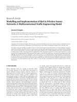
00.10.20.30.40.50.60.70.80.91
x
vs
0.2
0.3
0.4
0.5
0.6
0.7
0.8
0.9
1
x
sv
0dB
3dB
5dB
E
b
/N
0
= 5dB
E
b

/N
0
= 3dB
E
b
/N
0
= 0dB
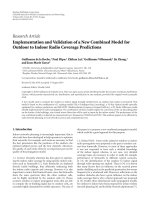
Figure 2: Mutual information evolution at the state-check node.
Comparison of the approximation methods with the exact mutual
information at the state-check node. The solid lines represent the
GA approximation, the broken lines the EC approximation, and
plus signs show Monte Carlo simulations.
It follows that
x
sv
=
1
2
x
sv
|
(+1,+1)
+
1
2
x
sv
|
(+1,−1)

=
1
3

1+x
vs

C
TIAWGNC
.
(20)
In Figure 2, we compare the two approximations for the
state node EXIT function with (14)and(20), for three dif-
ferent signal-to-noise ratios. The solid lines show the GA ap-
proximation whereas the broken lines show the EC approx-
imation. We have also indicated with plus signs the mutual
information obtained with Monte Carlo simulations. Our
numerical results show that the Gaussian a priori GA ap-
proximation is more attractive since the mutual information
computed under this assumption have the smallest gap to the
exact mutual information (Monte Carlo simulation without
any approximation).
4. LDPC CODE OPTIMIZATION
Using the EXIT charts for the LDPC codes [12, 15]andfor
the state-check node under the two considered approxima-
tions (14), (20), we are now able to give the evolution of
the mutual information x along a whole 2-user decoding
iteration. The irregularity of the LDPC code is defined as
usual by the degree sequences


{
λ
i
}
d
v
i=2
, {ρ
j
}
d
c
j=2

that repre-
sent the fraction of edges connected to variable nodes (resp.,
check nodes) of degree i (resp., j). As in the single-user case,
we wish to have an optimization algorithm that could be
solved quickly and efficiently using linear programming. In
ordertodoso,wemustmakedifferent assumptions that are
mandatory to ensure that the evolution of the mutual infor-
mation is linear in the parameters
{λ
i
}:
{H
0
} hypothesis equal LDPC codes. Under this hypothesis,
we assume that the 2 LDPC codes belong to the same
ensemble (

{λ
i
}
d
v
i=2
, {ρ
j
}
d
c
j=2
);
{H
1
} hypothesis without interleaver. Under this hypothesis,
each and every state-check node is connected to two
variable nodes (one in each LDPC code) having exactly
the same degree.
Proposition 2. Under hypotheses H
0
and H
1
, the evolution of
the mutual information x
vc
at the lth iteration under the paral-
lel s cheduling described in Sect ion 2 is linear in the parameters
{λ
i

}.
Proof. See Appendix C.
From Proposition 2, we can now write the evolution of
the mutual information for the entire graph. More precisely,
by using (12), (14), and (20), we finally obtain (21) for the
Gaussian approximation and (22) for the erasure channel ap-
proximation:
x
(l)
vc
=
d
v

i=2
λ
i
J

J
−1

1
2
J

F
+1,+1

iJ

−1

ρ

x
(l−1)
vc

, σ
2


+
1
2
J

F
+1,+1

iJ
−1

ρ

x
(l−1)
vc

, σ

2



+(i − 1)J
−1

ρ

x
(l−1)
vc


Δ
= F
GA

λ
i

, x
(l−1)
vc
, σ
2

,
(21)
x

(l)
vc
=
d
v

i=2
λ
i
J

J
−1

C
TIAWGNC
3

1+J

iJ
−1

ρ

x
(l−1)
vc




+(i − 1)J
−1

ρ

x
(l−1)
vc


Δ
= F
EC

λ
i

, x
(l−1)
vc
, σ
2

(22)
with
ρ

x
(l−1)

vc

=
1 −
d
c

j=2
ρ
j
J

( j − 1)J
−1

1 − x
(l−1)
vc


. (23)
It is interesting to note that, in (21)and(22), the evolution
of the mutual information is indeed linear in the parameters
{λ
i
}, when {ρ
j
} are fixed.
As often presented in the literature, we will only optimize
the data node parameters

{λ
i
}, for a fixed (carefully chosen)
check node degree distribution
{ρ
j
}. The optimization cri-
terion is to maximize R subject to a vanishing bit error rate.
The optimization problem can be written, for a given σ
2
and
agivenρ(x) as follows:
6 EURASIP Journal on Wireless Communications and Networking
maximize
d
v

i=2
λ
i
i
subject to

C
1

d
v

i=2

λ
i
= 1 [mixing constraint],

C
2

λ
i
∈ [0, 1] [proportion constraint],

C
3

λ
2
<
exp

1/

2σ
2


d
c
j=2
( j − 1)ρ
j

[stability constraint],

C
4

F

λ
i

, x, σ
2

>x,
∀x ∈ [0,1[ [convergence constraint],
(24)
where (C
3
) is the condition for the fixed point to be stable
(see Proposition 3)andwhere(C
4
) corresponds to the con-
vergence to the stable fixed point x
= 1, which corresponds
to zero error rate constraint.
Solution to the optimization problem
For a given σ
2
and a given ρ(x), the cost function and the
constraints (C

1
), (C
2
), and (C
3
) are linear in the par ameters
{λ
i
}. The function used in constraint (C
4
) is either (21)or
(22) which are both linear in the parameters
{λ
i
}. The op-
timization problem can then be solved for a given ρ(x)by
linear programming . We would like to emphasize the fact
that the hypotheses H
0
and H
1
are necessary to have a lin-
ear problem, which is the key feature of quick and efficient
LDPC optimization.
These remarks allow us to propose an algorithm that
solves the optimization problem (24)intheclassoffunctions
ρ(x) of the type ρ(x)
= x
n
,foralln>0.

(i) First, we fix a target SNR (or equivalently σ
2
).
(ii) Then, for each n>0, ρ(x)
= x
n
and we perform a lin-
ear programming in order to find a set of parameters
{λ
i
}that maximizes the rate under the constraints (C
1
)
to (C
4
)(24). In order to integrate the (C
4
) constraint
in the algorithm, we quantize x.Foreachquantized
value of x, the equation in (C
4
) leads to an additional
constraint. Hence, for each n,wegetarate.
(iii) Finally, we choose n that maximizes the rate (over all
n).
In practice, the search over all possible n is performed up
to a maximal value. This is to insure that the g raph remains
sparse.
Stability of the solution
Finally, the stability condition of the fixed point for the 2-

user MAC channel is given in the following proposition.
Proposition 3. The local stability condition of the DE for the
2-user Gaussian MAC is the same as that of the sing le user case:
λ
2
<
exp

1/

2σ
2


d
c
j=2
( j − 1)ρ
j
. (25)
The proof is given in Appendix D.
5. RESULTS
In this section we present results for codes designed accord-
ing to the two methods presented in Section 3,forratesfrom
0.3 to 0.6, and we compare the methods on the basis of the
true thresholds obtained by DE and finite length simulations.
Tabl e 1 shows the performance of LDPC codes optimized
with the Gaussian approximation. Ta bl e 2 shows the perfor-
mance of LDPC codes designed according to the Erasure
channel approximation. In both tables the code rate, the

check nodes degrees ρ(x)
=

d
c
j=2
ρ
j−1
j
, the optimized pa-
rameters
{λ
i
}
d
v
i=2
, and the gap to the 2-user Gaussian MAC
Shannon limit are indicated.
We can see that the LDPC codes optimized for the 2-
user MAC channel are indeed very good and have decoding
thresholds very close to the capacity. Our numerical results
show that, the Gaussian a priori approximation is more at-
tractive since the codes desig ned under this assumption have
the smallest g a p to Shannon limit.
An interesting result is that the codes obtained for R
=
0.3andR = 0.6 are worse than the ones obtained for R = 0.5.
Our opinion is that it does not come from the same reason.
For small rates (R

= 0.3), the multiuser problem is easy to
solve because the system load (sum rate) is lower than 1, but
the approximations of DE become less and less accurate as
the rate decreases. R
= 0.3 gives worse codes than R = 0.5
because of the LDPC part of the multiuser graph. For larger
rates (R
= 0.6), the DE approximations are fairly accurate,
but the multiuser problem we address is more difficult, as
the system load is larger than 1 (equal to 1.2). R
= 0.6gives
worse codes than R
= 0.5 because of the multiuser part of the
graph (state-check node).
In order to verify the asy m ptotical results obtained with
DE, we h ave made extensive simulations for a finite length
equal to N
= 50 000. The codes have been build with an ef-
ficient parity check matrix construction. Since the progres-
sive edge growth algorithm [16] tends to be inefficient at very
large code lengths, we used the ACE algorithm proposed in
[17] which helps to prevent the apparition of small cycles
with degree two bitnodes. The ACE algorithm generally low-
ers greatly the error flo or of very irregular LDPC codes (like
the ones in Tables 1 and 2).
Figure 3 shows the simulation results for three rates R
∈
{
0.3, 0.5, 0.6} and for the two different approximations of
the state-check node EXIT function presented in this paper:

GA and EC. The curves are in accordance with the threshold
computations, except the fact that codes optimized with the
EC approximation tend to be better than the GA codes for
the rate R
= 0.3. We confirm also the behavior previously
discussed in that the codes with R
= 0.5 are closer to the
Shannon limit than the codes with R
= 0.3andR = 0.6.
A. Roumy and D. Declercq 7
Table 1: Optimized LDPC codes for the 2-user Gaussian channel obtained with the Gaussian Approximation of the state-check node. The
distance between the (E
b
/N
0
) threshold δ (evaluated with true DE) and the Shannon limit S
l
is given in dBs.
GA
Rate 0.3 0.4 0.5 0.6
ρ(x) x
7
x
8
x
9
x
10
λ(x) λ
i

i λ
i
i λ
i
i λ
i
i
2.749809e − 01 2 2.786702e − 01 2 3.170178e − 01 2 4.393437e − 01 2
2.040936e − 01 3 2.306721e − 01 3 2.312804e − 01 3 1.305465e − 01 3
5.708851e − 03 4 5.059420e − 02 9 4.241393e − 02 17 2.508237e − 02 20
1.817382e − 02 5 4.229097e − 04 10 1.714436e − 01 18 2.462773e −01 21
1.891399e − 02 6 1.608676e − 01 12 2.378443e − 01 100 1.587501e − 01 100
2.682255e − 02 7 2.787730e − 01 100
7.317063e − 02 8
1.130643e − 01 13
2.650713e − 01 100
δ − S
l
0.22 0.15 0.19 0.52
Table 2: Optimized LDPC codes for the 2-user Gaussian channel obtained with the erasure channel approximation of the state-check node.
The distance between the (E
b
/N
0
) threshold δ (evaluated with true DE) and the Shannon limit S
l
is given in dBs.
EC
Rate 0.3 0.4 0.5 0.6
ρ(x) x

7
x
8
x
9
x
10
λ(x) λ
i
i λ
i
i λ
i
i λ
i
i
2.762791e − 01 2 2.792405e − 01 2 3.165084e − 01 2 4.388191e − 01 2
2.321906e − 01 3 2.456371e − 01 3 2.339989e − 01 3 1.303074e − 01 3
7.870900e − 02 9 1.020663e − 01 13 4.285469e − 02 18 1.649224e −01 20
1.077795e − 01 10 8.130383e − 02 14 1.713483e − 01 19 1.093493e − 01 21
3.050418e − 01 100 2.917522e − 01 100 2.352897e −01 100 1.566018e − 01 100
δ − S
l
0.38 0.26 0.21 0.59
6. CONCLUSION
This paper has tackled the optimization of LDPC codes for
the 2-user Gaussian MAC and has shown that it is possi-
ble to design good irregular LDPC codes with very simple
techniques, the optimization problem being solved by linear
programming. We h ave proposed 2 different analytical ap-

proximations of the state-check node update, one based on
a Gaussian approximation and one very simple based on an
erasure channel approach. The codes obtained have decoding
thresholds as close as 0.15 dB away from the Shannon limit,
and can be used as initial codes for more complex optimiza-
tion techniques based on true density evolution. Future work
will deal with the generalization of our approach to more
thantwousersand/oruserswithdifferent powers.
APPENDICES
A. COMPUTATION OF FUNCTIONS F
+1,+1
AND F
+1,−1
We proceed to compute the state-check node update rule for
the mean of the messages.
Let us first consider hypothesis Z
= [+1, +1]
T
. Under the
Gaussian assumption, the conditional input distributions are
y
|
(+1,+1)
∼ N

2, σ
2

,
m

vs
|
(+1,+1)
∼ N

μ
vs
,2μ
vs

.
(A.1)
Therefore
m
vs
+
2y
− 2
σ
2




(+1,+1)
∼ N

μ
vs
+

2
σ
2
,2μ
vs
+
4
σ
2

,
m
vs
+
2y +2
σ
2




(+1,+1)
∼ N

μ
vs
+
6
σ
2

,2μ
vs
+
4
σ
2

.
(A.2)
Since for a Gaussian random variable x ∼ N (μ + a,2μ + b),
where a and b are real valued constants,
E

log

1+e
±x

=
1
√
π

+∞
−∞
e
−z
2
log


1+e
±(
√
4μ+2bz+μ+a)

dz
(A.3)
8 EURASIP Journal on Wireless Communications and Networking
00.511.522.533.54 4.55
E
b
/N
0
10
−6
10
−5
10
−4
10
−3
10
−2
10
−1
10
0
Bit error rate
EC approximation
GA approximation

R
= 0.3 R = 0.5 R = 0.6
S
l
(0.3) S
l
(0.5)
S
l
(0.6)
Figure 3: Simulation results for the optimized LDPC codes given
in Tables 1 and 2. The codeword length is N
= 50 000. The maxi-
mum number of iterations is set to 200. For comparison, we have
indicated the Shannon limit for the three considered rates.
and by using (9), we get
E

m
sv
| Z = [+1, +1]
T

=−
μ
vs
+
1
√
π


+∞
−∞
e
−z
2
log

1+e
+2
√
μ
vs
+(2/σ
2
)z+μ
vs
+2/σ
2
1+e
−2
√
μ
vs
+(2/σ
2
)z−μ
vs
−6/σ
2


dz
= F
+1,+1

μ
vs
, σ
2

.
(A.4)
Similarly we get F
+1,−1
(μ
vs
, σ
2
).
B. PROOF OF PROPOSITION 1
To prove Proposition 1, we first need to show the following
lemmas.
Lemma 1. Consider a state-check node. Assume a symmetric
input message and a symmetric channel obser vation. The out-
put message is symmetric.
Proof of Lemma 1. We consider a state- check node that veri-
fies the symmetry condition (see Definition 1). Without loss
of generality we can assume k to be the output user and j the
input user.
Let y (z, resp.) denote the observation vector when the

codewords x
[k]
, x
[ j]
(−x
[k]
, −x
[ j]
, resp.) are sent. Now note
that a symmetric-output 2-user MAC can be modeled as fol-
lows (see [10, Lemma 1]):
y
=−z (B.1)
since p

y
t
| x
[k]
t
, x
[ j]
t

= p

− y
t
|−x
[k]

t
, −x
[ j]
t

and since we
are interested in the performance of the BP algorithm, that
is, the densities of the messages.
Similarly we denote by m
[ j]
t
, m
[k]
t
(r
[ j]
t
, r
[k]
t
, resp.) the in-
put and output messages of the state-check node at position
t when the codewords x
[k]
, x
[ j]
(−x
[k]
, −x
[ j]

,resp.)aresent.
Let us assume a symmetric input message, that is,
p

m
[ j]
t
| x
[ j]
t

=
p

−m
[ j]
t
|−x
[ j]
t

.Hereagainwecanmodel
this input message as
m
[ j]
t
(y) =−r
[ j]
t
. (B.2)

The state-check node update rule is denoted by
Ψ
S

y
t
, m
[ j]
t

.
The output message verifies
m
[k]
t
= Ψ
S

y
t
, m
[ j]
t

=
Ψ
S

−
z

t
, −r
[ j]
t

=−
Ψ
S

z
t
, r
[ j]
t

=−
r
[k]
t
(z),
(B.3)
where the second equation is due to the symmetry conditions
of the channel and the input message and the third equation
follows from the symmetry condition of the state-check node
map.
This can be rewritten as
p

m
[k]

t
| x
[k]
t
, x
[ j]
t

=
p

−
m
[k]
t
|−x
[k]
t
, −x
[ j]
t

(B.4)
and therefore
p

m
[k]
t
| x

[k]
t

=
p

−
m
[k]
t
|−x
[ j]
t

(B.5)
by marginalizing the probability with respect to x
[ j]
t
and by
using (B.4).
Equation (B.5) implies that with symmetric observ ation
and symmetric input message, the message at the state-check
node output is also symmetric. The symmetry is conserved
through the state-check node which completes the proof of
Lemma 1.
Lemma 2. Consider a state-check node. Assume a symmetric
channel observation. At any iteration, the input and output
messages of the state check node are sy mmetric s.
Proof of Lemma 2. Lemma 1 shows that the state check node
conserves the symmetry condition, [10, Lemma 1] shows

the conservation of the symmetry condition of the messages
through the variable and check node. At initialization, the
channel observation is symmetric therefore a proof by induc-
tion shows the conservation of the symmetry property at any
iteration with a BP decoder.
Proof of Proposition 1. A consequence of Lemma 1 is that the
number of cases that need to be considered to determine the
entire average behavior of the state-check node can be di-
vided by a factor 2. We can assume that the all-one sequence
is sent for the output user. However, all the sequences of the
input user need to be considered and therefore on the aver-
age we can assume an input sequence with half symbols fixed
at “1” and half symbols at “
−1.”
A. Roumy and D. Declercq 9
C. PROOF OF PROPOSITION 2
Lemma 3. Under the parallel scheduling assumption desc ribed
in Section 2 and by using hypothesis H
0
(see Section 4), the en-
tire behavior of the BP decoder can be predicted with one de-
coding iteration (i.e., half of a round).
Proof of Lemma 3. Under the parallel scheduling assumption
described in Section 2, two decoding iterations (one for e ach
user) are completed simultaneously. Hence by using hypoth-
esis H
0
(same code family for both users), the two de-
coding iterations are equivalent in the sense that they pro-
vide messages with the same distribution. This can be eas-

ily shown by induction. It follows that a whole round is en-
tirely determined by only one decoding iteration (i.e., half of
a round).
Therefore in the following we omit the user index.
Proof of Proposition 2. We now proceed to compute the evo-
lution of the mutual information through all nodes of the
graph. By assuming that the distributions at any iteration are
Gaussian, we obtain similarly to method 1 in [12] the mutual
information evolutions as
x
(l)
vc
=
d
v

i=2
λ
i
J

J
−1

x
(l−1)
sv

+(i − 1)J
−1


x
(l−1)
cv


,
x
(l)
cv
= 1 −
d
c

j=2
ρ
j
J

( j − 1)J
−1

1 − x
(l−1)
vc


,
x
(l)

vs
=
d
v

i=2

λ
i
J

iJ
−1

x
(l)
cv


,
x
(l)
sv
= f

x
(l)
vs
, σ
2


,
(C.1)
where

λ
i
denotes the frac tion of variable nodes of degree i
(

λ
i
= (λ
i
/i)/(

j
λ
j
/j)) and where
f

x
sv
, σ
2

=
1
2

x
sv
|
(+1,+1)
+
1
2
x
sv
|
(+1,−1)
(C.2)
with x
sv
defined either in (14)or(20), depending on the ap-
proach used.
First notice that this system is not linear in the parameters
{λ
i
}. But by using hypothesis H
1
, the input message m
sv
of
avariablenodeofdegreei results from a variable node with
the same degree. It follows that the third equation in (C.1)
reduces to
x
(l)
vs

= J

iJ
−1

x
(l)
cv


. (C.3)
Finally the global recursion in the form (21)-(22)isob-
tained by combining all four equations and the global recur-
sion is linear in the paremeters
{λ
i
}.
D. PROOF OF PROPOSITION 3
Similarly to the definition of the message (see Section 2)and
of the mutual information (see Section 3), we will denote by
P
(l)
ab
the distribution of the messages from node a to node b
in iteration l, where (a, b) can either be v for variable node, c
for check node, or s for state-check node.
We follow in the footsteps of [18] and analyze the local
stability of the zero error rate fixed point by using a small
perturbation approach. Let us denote by Δ
0

the dir ac at 0,
that is, the distribution with 0.5-BER and Δ
+∞
the distribu-
tion w ith zero-BER when the symbol “+1” is sent.
From Lemma 3 (see Appendix C) we know that only half
of a complete round needs to be performed in order to get
the entire behavior of the BP decoder. All distributions of the
DE are conditional densities of the messages given that the
symbol sent is +1. From the symmetry property of the vari-
able and check nodes, the transformation of the distributions
can be performed under the assumption that the all-one se-
quence is sent. However, for the state-check node, different
cases will be considered as detailed below.
We consider the DE recursion with state variable of the
dynamical system P
vc
. In order to study the local stability of
the fixed point Δ
∞
, we initialize the DE recursion at the point
P
(0)
vc
= (1 − 2)Δ
∞
+2Δ
0
(D.1)
for some small

 > 0, and we apply one iteration of the DE
recursion. Following [18] (and also in [12]), the distribution
P
(0)
cv
can be computed which leads to P
(0)
vs
as
P
(0)
vs
= Δ
∞
+ O


2

. (D.2)
For the sake of brevity, we omit the now-well-known step-
by-step derivation and focus on the transformation at the
state-check node. Note that (D.2) holds with and without the
hypothesis H
1
(without interleaver) since it follows from the
fact that an i-fold convolution of the distribution P
(0)
cv
is per-

formed with i
≥ 2inbothcases.
From the symmetry property (see Proposition 1) of the
state check node, the entire behavior at a state-check node
can be predicted under the two hypotheses called (+1, +1)
and (+1,
−1), that is, when the output symbol is +1 and when
the input symbol is either +1 or
−1 with probability 1/2each.
In the following, we seek for the output distribution P
(0)
sv
,
for a given input distribution P
(0)
vs
(conditional distribution
given that the input symbol is +1) and a given channel dis-
tribution.
Hypothesis (+1, +1) w.p. 1/2. From (D.2)and(5)weget
m
(0)
vs
∼ P
(0)
vs
= Δ
∞
+ O



2

,
y ∼ N

2, σ
2

.
(D.3)
Hence, by applying (4)wehave
m
(0)
sv
=
2+2y
σ
2
∼ N

2
σ
2
,
4
σ
2

. (D.4)

Hypothesis (+1,
−1) w.p. 1/2. From (D.2) and from the
symmetry property of the input message at the state-check
node, we have
m
(0)
vs
∼ P
(0)
vs
(−z) = Δ
−∞
+ O


2

(D.5)
10 EURASIP Journal on Wireless Communications and Networking
and from (5)weget
m
(0)
vs
∼ Δ
−∞
+ O


2


,
y ∼ N

0, σ
2

.
(D.6)
Hence, by applying (4)wehave
m
(0)
sv
=
−
2y − 2
σ
2
∼ N

2
σ
2
,
4
σ
2

. (D.7)
Combining (D.4)and(D.7), we obtain
P

(0)
sv
= N

2
σ
2
,
4
σ
2

. (D.8)
It follows that at convergence, the channel seen by one user
is P
(0)
sv
which is exactly the LLR distribution of a BIAWGNC
with noise variance σ
2
. It follows that at convergence the DE
recursion is equivalent to the single-user case and the stabil-
ity condition is therefore [18]
λ
2
<
exp

1/


2σ
2


d
c
j=2
( j − 1)ρ
j
. (D.9)
REFERENCES
[1] B. Rimoldi and R. Urbanke, “A rate-splitting approach to the
Gaussian multiple-access channel,” IEEE Transactions on Infor-
mation Theory, vol. 42, no. 2, pp. 364–375, 1996.
[2] R. Ahlswede, “Multi-way communication channels,” in Pro-
ceedings of the 2nd IEEE International Symposium on Informa-
tion Theory (ISIT ’71), pp. 23–52, Aremenian Prague, Czech
Republic, 1971.
[3] H. Liao, Multiple access channels, Ph.D. thesis, University of
Hawaii, Honolulu, Hawaii, USA, 1972.
[4] R. Palanki, A. Khandekar, and R. McEliece, “Graph based
codes for synchronous multiple access channels,” in Proceed-
ings of the 39th Annual Allerton Conference on Communication,
Control, and Computing, Monticello, Ill, USA, October 2001.
[5] A. Amraoui, S. Dusad, and R. Urbanke, “Achieving general
points in the 2-user Gaussian MAC without time-sharing
or rate-splitting by means of iterative coding,” in Proceed-
ings of IEEE International Symposium on Information Theory
(ISIT ’02), p. 334, Lausanne, Switzerland, June-July 2002.
[6] A. De Baynast and D. Declercq, “Gallager codes for multiple

user applications,” in Proceedings of IEEE International Sym-
posium on Information Theory (ISIT ’02), p. 335, Lausanne,
Switzerland, June-July 2002.
[7] F. R. Kschischang, B. J. Frey, and H A. Loeliger, “Factor graphs
and the sum-product algorithm,” IEEE Transactions on Infor-
mation Theory, vol. 47, no. 2, pp. 498–519, 2001.
[8] J. Pearl, Probabilistic Reasoning in Intelligent Systems: Networks
of Plausible Inference, Morgan Kaufmann, San Mateo, Calif,
USA, 1988.
[9] R. M. Tanner, “A recursive approach to low complexity codes,”
IEEE Transactions on Information Theory,vol.27,no.5,pp.
533–547, 1981.
[10] T. J. Richardson and R. Urbanke, “The capacity of low-density
parity-check codes under message-passing decoding,” IEEE
Transactions on Information Theory, vol. 47, no. 2, pp. 599–
618, 2001.
[11] S. Ten Brink, “Designing iterative decoding schemes with the
extrinsic information transfer chart,” International Journal of
Electronics and Communications, vol. 54, no. 6, pp. 389–398,
2000.
[12] A. Roumy, S. Guemghar, G. Caire, and S. Verd
´
u, “Design
methods for irregular repeat-accumulate codes,” IEEE Trans-
actions on Information Theory, vol. 50, no. 8, pp. 1711–1727,
2004.
[13] A. Bennatan and D. Burshtein, “On the application of LDPC
codes to arbitrary discrete-memoryless channels,” IEEE Trans-
actions on Information Theory, vol. 50, no. 3, pp. 417–438,
2004.

[14] C C. Wang, S. R. Kulkarni, and H. V. Poor, “Density evolution
for asymmetric memoryless channels,” IEEE Transactions on
Information Theory, vol. 51, no. 12, pp. 4216–4236, 2005.
[15] S Y. Chung, T. J. Richardson, and R. Urbanke, “Analysis of
sum-product decoding of low-density parity-check codes us-
ing a Gaussian approximation,” IEEE Transactions on Informa-
tion Theory, vol. 47, no. 2, pp. 657–670, 2001.
[16] X Y. Hu, E. Eleftheriou, and D M. Ar nold, “Progressive edge-
growth tanner graphs,” in Proceedings of IEEE Global Telecom-
munications Conference (GLOBECOM ’01), vol. 2, pp. 995–
1001, San Antonio, Tex, USA, November 2001.
[17] T.Tian,C.Jones,J.D.Villasenor,andR.D.Wesel,“Construc-
tion of irregular LDPC codes with low error floors,” in Pro-
ceedings of IEEE International Conference on Communications
(ICC ’03), vol. 5, pp. 3125–3129, Anchorage, Alaska, USA, May
2003.
[18] T.J.Richardson,M.A.Shokrollahi,andR.Urbanke,“Design
of capacity-approaching irregular low-density parity-check
codes,” IEEE Transactions on Information Theory, vol. 47, no. 2,
pp. 619–637, 2001.