Báo cáo hóa học: " Research Article On Intercell Interference and Its Cancellation in Cellular Multicarrier CDMA Systems Simon Plass German Aer" potx

Hindawi Publishing Corporation
EURASIP Journal on Wireless Communications and Networking
Volume 2008, Article ID 173645, 11 pages
doi:10.1155/2008/173645
Research Article
On Intercell Interference and Its Cancellation in
Cellular Multicarrier CDMA Systems
Simon Plass
German Aerospace Center (DLR), Institute of Communications and Navigation, Oberpfaffenhofen, 82234 Wessling, Germany
Correspondence should be addressed to Simon Plass,
Received 2 May 2007; Accepted 17 September 2007
Recommended by Luc Vandendorpe
The handling of intercell interference at the cell border area is a strong demand in future communication systems to guarantee effi-
cient use of the available bandwidth. Therefore, this paper focuses on the application of iterative intercell interference cancellation
schemes in cellular multicarrier code division multiple access (MC-CDMA) systems at the receiver side for the downlink. First,
the influence of the interfering base stations to the total intercell interference is investigated. Then, different concepts for intercell
interference cancellation are described and investigated for scenarios with several interfering cells. The first approach is based on
the use of the hard decision of the demodulator to reconstruct the received signals. This does not require the higher amount of
complexity compared to the second approach which is based on the use of the more reliable soft values from the decoding process.
Furthermore, the extrinsic information as a reliability measure of this soft iterative cancellation process is investigated in more de-
tail based on the geographical position of the mobile terminal. Both approaches show significant performance gains in the severe
cell border area. With the soft intercell interference cancellation scheme, it is possible to reach the single-user bound. Therefore,
the intercell interference can be almost eliminated.
Copyright © 2008 Simon Plass. This is an open access article distributed under the Creative Commons Attribution License, which
permits unrestricted use, distribution, and reproduction in any medium, provided the original work is properly cited.
1. INTRODUCTION
The high data rate demands of next generation mobile com-
munication systems require a very efficient exploitation of
the available spectrum. Therefore, future cellular mobile
concepts reuse the whole spectrum in each served cell [1]
which corresponds to a frequency reuse of one. By applying

the same frequency band in neighboring cells, the cell bor-
der areas are highly influenced by intercell interference. This
causes severe performance degradations or even connection
loss.
Technologies which are currently considered candidates
for these future communication systems are based on the
generalized multicarrier (GMC) concept [2, 3]. The technol-
ogy multicarrier code division multiple access (MC-CDMA)
[4, 5] is within the GMC concept and combines the bene-
fits of multicarrier transmission and spread spectrum. Mul-
ticarrier transmission, namely, orthogonal frequency divi-
sion multiplexing (OFDM) [6], offers simple digital realiza-
tion due to the fast Fourier transformation (FFT) operation
and low complex receivers. Additionally, spread spectrum,
namely code division multiple access (CDMA), gives high
flexibility, robustness, and frequency diversity gains [7]. Re-
cently, the cellular aspects of MC-CDMA were investigated.
In [8, 9], first analyses regarding the intercell interference
modeling for cellular MC-CDMA environments are given. A
Gaussian approximation was proposed for the intercell inter-
ference modeling which was verified with more analytical in-
vestigations in [10, 11]. This simplified intercell interference
assumption allows a large reduction of the simulation com-
plexity for cellular MC-CDMA systems. In [12, 13] the main
focus was on the overall performance of an MC-CDMA sys-
tem in a cellular environment. It was shown that there exist
large performance degradations in the cell border area. Even
a sectorized cellular system could not reduce these degrada-
tions [14].
Theoretically, gains from using intercell interference

avoidance schemes are large [15], but maximal gains would
require fast and tight intercell coordination. For example,
frequency partitioning in cellular networks on a slower time
scale has for a long period received interest [16]aswellasthe
useofpowercontrol[17], dynamic channel assignment, and
2 EURASIP Journal on Wireless Communications and Networking
channel borrowing. Note that the packet-switched channel-
aware scheduled transmissions which will take place in future
systems complicate the use of many of the previously sug-
gested schemes for intercell interference avoidance. For ex-
ample, it is not, without additional side information, possi-
ble to conclude that the interference power in a set of sub-
carriers is likely to be higher/lower than average just be-
cause it is measured as high/low at present. Therefore, due
to the orthogonal spread data symbols and the resulting re-
dundancy in the transmission the spread spectrum technique
MC-CDMA provides the possibility to iteratively remove the
intercell interference at the receiver side without the need
of high complex intercell interference management schemes
from the network side.
This paper presents iterative intercell interference cancel-
lation schemes for a cellular MC-CDMA downlink. An in-
tercell interference cancellation (ICIC) scheme was already
proposed in [18] by taking into account the hard decisions
from the demodulator to reconstruct the signal and cancel
the intercell interference. In this paper, we propose to use ad-
ditional signal power information for the cancellation pro-
cess which improves this hard ICIC process. More reliable
information are the soft values from the outer channel de-
coder. Within a single MC-CDMA link the soft information

is already used for iterative cancellation of the multiple access
interference (MAI) [19]. It is possible to extend this principle
to a cellular MC-CDMA downlink to cancel the intercell in-
terference with a soft ICIC [20, 21]. Most cellular interference
investigations on the link level are based on one interfering
cell [8, 10, 12, 18, 20, 21] due to complexity constraints. This
paper studies the influence of a cellular environment with a
whole tier of interfering base stations around the desired base
station. The extrinsic information of the decoding process is
considered as a degree of reliability for the soft ICIC process.
In the following section, we first introduce the cellular
MC-CDMA system and its cellular environment. Section 3
proposes different approaches of ICIC techniques. First, the
hard decisions from the demodulator are used for the hard
ICIC process. Further, an iterative ICIC technique based on
soft values is presented in more detail which is named soft
ICIC. The influence of intercell interference within a cellular
environment is investigated in Section 4. Also in this section,
the performances of the different ICIC schemes are com-
pared by simulations.
2. CELLULAR MC-CDMA SYSTEM
2.1. MC-CDMA Transmitter
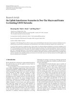
The MC-CDMA transmitter is shown in Figure 1. The sys-
tem contains N
c
subcarriers for N
u
users. A channel-coder
encodes the bit stream of each user. The encoded bits are in-
terleaved by the outer interleaver Π

out
and the interleaved
code bits c
(n)
of user n are passed to the symbol modula-
tor. With respect to different modulation alphabets (e.g., PSK
or QAM), the bits are modulated to complex-valued data
symbols with the chosen cardinality. Before each modulated
signal can be spread with a Walsh-Hadamard sequence of
length L
≥ N
u
, a multiplexer (MUX) arranges the signals
to N
d
≤ N
c
/L parallel data symbols per user. For the case
that N
d
= N
c
/L, the data stream is distributed over all avail-
able subcarriers. On the other hand, if N
d
<N
c
/L, other data
streams are assigned to the remaining subcarriers, which are
named user groups [7] and are independent from the afore-

mentioned data stream. This guarantees equally loaded sub-
carriers. The kth symbol of all users, d
k
= [d
(1)
k
, , d
(N
u
)
k
]
T
,
is multiplied with an L
×N
u
spreading matrix C
L
resulting in
s
k
= C
L
d
k
, s
k
∈ C,1≤k ≤ N
d

. (1)
In an MC-CDMA system, the system load is N
u
/L and
can be set to a value ranging from 1/L to 1. For maximizing
the diversity gain, the block s
= [s
1
, , s
N
d
]
T
is frequency-
interleaved by the inner random interleaver Π
in
which rep-
resents one OFDM symbol. By taking into account a whole
OFDM frame the interleaving can be done in two dimension,
that is, time and frequency. X
(m)
l,i
denotes the value of the lth
OFDM symbol in the ith subcarrier at base station (BS) m
out of N
BS
. Furthermore, N
s
OFDM symbols describe one
OFDM frame whereby each OFDM symbol has N

c
subcarri-
ers.
An OFDM modulation is performed on each block and
contains operations as follows. First, an inverse FFT (IFFT)
with N
FFT
≥ N
c
points is done. Thus, the time domain sig-
nal is given by x
(m)
l,n
= IFFT{X
(m)
l,i
},wheren = 1, , N
FFT
.
Then, a guard interval (GI) in form of a cyclic prefix is in-
serted having N
GI
samples. At the end of the transmitter a
D/Aconversioniscarriedoutandx
(m)
(t) is obtained.
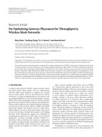
2.2. Cellular MC-CDMA receiver
Figure 2 depicts the receiver structure of the MC-CDMA sys-
tem. The signal x
(m)

(t) is transmitted over a mobile radio
channel and y(t) is received. Then the inverse OFDM is per-
formed including the removing of the GI and the FFT. We
assume for the channel fading a quasi-static fading process,
that is, the fading is constant for the duration of one OFDM
frame. With this quasi-static channel assumption the well-
known description of OFDM in the frequency domain is
given.
After OFDM demodulation of the OFDM symbol, the re-
ceived signal is
Y
l,i
=
N
BS
−1

m=0
X
(m)
l,i
H
(m)
l,i
+ N
l,i
,(2)
where H
(m)
l,i

is the channel transfer function and N
l,i
is the
additive white Gaussian noise (AWGN) with zero mean and
variance N
0
.
The inner deinterleaver Π
−1
in
and a parallel-to-serial con-
verter arranges the received signal to the kth spread symbol
of the N
u
users r
k
= [r
k,1
, , r
k,L
]
T
. The entries of the de-
spreader results from the linear minimum mean-squared er-
ror (MMSE) one tap equalizer G which restores the lost or-
thogonality between the spreading codes. Within a cellular
Simon Plass 3
User 1
User N
u

COD Π
out
c
(1)
Mod
.
.
.
.
.
.
.
.
.
COD
Π
out
c
(N
u
)
Mod
MUX
d
(1)
1
.
.
.
d

(N
u
)
1
d
(1)
N
d
.
.
.
d
(N
u
)
N
d
C
L
.
.
.
C
L
+
+
s
1
.
.

.
s
N
d
S/P
Π
in
X
(m)
l,i
.
.
.
X
(m)
l,N
c
IFFT
GI D/A
x
(m)
(t)
Figure 1: MC-CDMA transmitter of the mth base station.
y(t)
A/D GI
−1
FFT
.
.
.

Y
l,i
Y
l,N
c
Π
−1
in
.
.
.
P/S
r
1
r
N
d
Eq
.
.
.
Eq
C
H
L
.
.
.
C
H

L

d
1
.
.
.

d
N
d
S/P
DMUX
.
.
.
Demod
Demod
q
1
q
N
u
Π
−1
out
.
.
.
Π

−1
out
DEC
.
.
.
DEC
User 1
User N
u
Figure 2: MC-CDMA receiver.
environment the MMSE has to be modified [11], resulting in
the diagonal matrix entries
G
i,i
=
H
(m)∗
l,i


H
(m)
l,i


2
+ σ
2
+


N
BS
−1
m

=0
m

=m
E



X
(m

)
l,i
H
(m

)
l,i


2

,(3)
where σ

2
= (L/N
u
)( N
0
/E
s
) is the actual variance of the noise
and

N
BS
−1
m

=0,m

=m
E{|X
(m

)
l,i
H
(m

)
l,i
|
2

} is the total power of the
intercell interference. (
·)
∗
denotes for complex conjugation.
Therefore, the data symbols for the demodulator process re-
sult in
d
k
= C
H
L
Gr
k
=


d
(1)
k
, ,

d
(N
u
)
k

T
. (4)

All symbols of the desired user

d
(1)
k
are combined to a
serial data stream. Without loss of generality, we skip the
symbol and user indices k and n for notational convenience
in the following. The symbol demodulator demodulates the
data symbols to real-valued soft-decisions q. In addition, it
calculates the log-likelihood ratio (LLR) [22]foreachcode
bit c by
L(c)
= log
P

c = 0 |

d

P

c = 1 |

d

. (5)
The sign of L(c) is the hard decision and the magnitude
|L(c)| is the reliability of the decision. The code bits are dein-
terleaved and decoded using the MAX-Log-MAP algorithm

[23] which generates the LLR
L(c
| q) = log

P(c = 0 | q)
P(c = 1 | q)

. (6)
In contrast to (5), the LLR value L(c
|q) is the estimate of all
bits in the coded sequence q [19].
r
α
d
0
MT
BS
(0)
BS
(I,2)
BS
(I,3)
BS
(I,4)
BS
(I,5)
BS
(I,6)
BS
(I,1)

Figure 3: Cellular environment.
Another degree of reliability of the decoder output can
begivenbytheexpectationofE
{c|q}, the so-called soft bits
[19, 24] which are defined by
λ(c
|q) = (+1)·P(c = 0 | q)+(−1)·P(c = 1 | q)
= tanh

L(c | q)/2

.
(7)
These soft bits are in the range of [
−1, +1]. The closer to the
minimum or maximum, the more reliable the decoded bits
are. There exists no reliable decision for λ(c
| q) = 0.
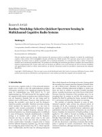
2.3. Cellular setup
We consider a synchronized cellular system in time and fre-
quency. The mth BS has a distance d
m
to the desired mobile
terminal (MT) and the BSs are distributed in a hexagonal
grid. We assume a normalized cell radius of one, and there-
fore, the distance is d
0
= 1forα = 30
◦
. The cellular setting is

illustrated in Figure 3.
The slowly varying signal power attenuation due to path
loss is generally modeled as the product of the γth power of
4 EURASIP Journal on Wireless Communications and Networking
distance d
m
and a log-normal component representing shad-
owing losses [25]. γ represents the path loss factor and η
m
is the Gaussian-distributed shadowing factor. Depending on
the position of the MT the carrier-to-interference ratio (C/I)
variesandisdefinedby
C
I
=
E



X
(0)
l,i
·H
(0)
l,i
·d
−γ
0
·10
η

0
/10 dB


2


N
BS
−1
m
=1
E



X
(m)
l,i
·H
(m)
l,i
·d
−γ
m
·10
η
m
/10 dB



2

. (8)
3. INTERCELL INTERFERENCE CANCELLATION
In this section we introduce different ICIC strategies. For
most of interference cancellation schemes additional infor-
mation is needed at the receiver. The receiver needs a de-
tectable signaling from the involved BSs which can be given
by an orthogonal signaling between the BSs. Further, a chan-
nel estimation process is needed for all impinging signals. On
the other side, intercell interference cancellation schemes at
the receiver avoid large configurations to reduce the intercell
interference at the transmitter side, namely, the base stations
and network. In the following, the concepts of hard and soft
ICICs are introduced which try to remove the interfering sig-
nals from the desired signal. This can guarantee a more suc-
cessful final decoding of the desired signal.
3.1. Hard ICIC
A first approach of ICIC is based on the use of the hard out-
put of the demodulator at the receiver to reproduce the in-
terfering or desired signals

Y
(m)
. We name this process hard
ICIC. In [18] three different combinations of the hard ICIC
are proposed. Simplified block diagrams of the hard ICIC
and its combinations are shown in Figures 4(a) and 4(b).
Without loss of generality, we skip the subcarrier and time

indices l and i for notational convenience in the following.
We extend the already proposed hard ICIC concepts to more
than one interfering cell. This is done by parallel processing
of the reconstruction of the interfering signals (m
= 0). All
blocks are set up with their specific cell parameters. First, the
direct hard ICIC (D-ICIC) with output

Y
D
= Y −
N
BS
−1

m=1

Y
(m)
(9)
can be seen as the basic concept block. Note that for the D-
ICIC the processing of the interfering cells (m
= 0) is used.
The indirect hard ICIC (I-ICIC) tries to reconstruct the de-
sired signal first and then the interfering signals. It should be
mentioned that the estimated interfering signals will be sub-
tracted in the final step from the received signal Y in contrast
to Figure 4(b). Therefore, the I-ICIC calculates

Y

I
= Y −
N
BS
−1

m=1

Y
(m)

Y
(0)
, (10)
Y
Π
−1
in
Equalizer
Despreader
Demod
Mod
Spreader
Π
in
H
(m)

Y
(m)

Hard ICICCell m
N
BS
−1

m

=
0
m

=
m
E{X
(m

)
H
(m

)
}
(a) Concept of the hard ICIC
Y
Hard ICIC
cell m
= 0

Y
(0)

−
+

Y
D
Parallel
hard ICICs
cells m
= 0
+
× +
−

Y
M
1/2
Indirect hard ICIC
Direct hard ICIC
Mean hard ICIC
Parallel
hard ICICs
cells m
= 0
N
BS
−1

m=1

Y

(m)
(b) Combinations of hard ICICs
Figure 4: Concept and combination of the hard ICIC.
where

Y
(m)

Y
(0)
represents the estimates depending on the first
estimate

Y
(0)
= Y −

Y
(0)
.Themean hard ICIC (M-ICIC)
combines the D-ICIC and I-ICIC concepts by

Y
M
= Y −0.5

N
BS
−1


m=1

Y
(m)

Y
(0)
+
N
BS
−1

m=1

Y
(m)

. (11)
All three concepts try to remove the intercell interference sig-
nals from the desired signal. In the final step, the output of
the hard ICIC is taken to be demodulated and decoded.
Due to the use of orthogonal signaling between the cells,
pilot signals can be used to achieve the received signal power,
for example, if the communication system is sufficiently syn-
chronized. Therefore, we propose to use this information for
the equalization process (cf. (3)) in all ICIC concepts (cf.
Figure 4(a)) which should influence and improve the over-
all performance of the hard ICICs.
3.2. Soft ICIC
A more sophisticated approach to cancel the intercell inter-

ference is based on the use of the more reliable soft val-
ues. In the following, we describe a soft ICIC technique for
an arbitrary number of interfering cells. Figure 5 shows the
block diagram of the proposed soft ICIC. The received signal
Simon Plass 5
Y
+
−
Y
des
Π
−1
in
Equalizer
Despreader
Demod +
−
L
E
Demod
L
A
Demod
Π
−1
out
L
A
Decod
Decod

b

Y
des
H
(0)
Π
in
Spreader
Mod
Π
out
L
E
Decod
+
−
Desired cell
Y
(m

)
int

Y
(m

)
int
+

−
−
+
+
Reconstruction of other interfering cells
m

= m
+
−
Y
(m)
int
Π
−1
in
Equalizer
Despreader
Demod
+
−
Π
−1
out
Decod
H
(m)
Π
in
Spreader

Mod
+
−
Π
out
Interfering cell m

Y
(m)
int
Figure 5: Concept of soft ICIC.
Y is processed as described in Section 2.2 in respect to its
specific cell parameters m for the desired and intercell in-
terference signals in parallel. In contrast to the hard ICIC
process, the demodulator computes from the received sym-
bols soft-demodulated extrinsic log-likelihood ratio values
L
E
Demod
. Unlike (5) without the use of a priori knowledge, the
demodulator, and therefore, L
E
Demod
exploits the knowledge
of a priori LLR-values L
A
Demod
with
L
A

Demod
= log
P(c
= 0)
P(c = 1)
(12)
coming from the decoder. L
E
Demod
is given by
L
E
Demod
(c) = log
P

c = 0 |

d,L
A
Demod
(c)

P

c = 1 |

d,L
A
Demod

(c)

−
L
A
Demod
(c). (13)
In the initial iteration, the LLR-values L
A
Demod
for the demod-
ulator are set to zero. After deinterleaving, the extrinsic LLR-
values L
E
Demod
become the a priori LLR-values L
A
Decod
of the
channel decoder. The channel decoder computes for all code
bits the a posteriori LLR-values L(c
| q) using the MAX-Log-
MAP algorithm (cf. (6)) and the extrinsic information L
E
Decod
is given by
L
E
Decod
= L(c | q) −L

A
Decod
. (14)
The extrinsic LLR-values L
E
Decod
are then interleaved to be-
come the a priori LLR-values L
A
Demod
used in the next itera-
tion in the demodulator. The signals of the desired cell

Y
des
and the interfering cells

Y
(m)
int
are reconstructed and for the
next iteration step the inputs of the processing blocks are
Y
des
= Y −
N
BS
−1

m=1


Y
(m)
int
,
Y
(m)
int
= Y −


Y
des
+
N
BS
−1

m

=1
m

=m

Y
(m

)
int


.
(15)
The iterative cancellation process requires high computa-
tional complexity at the receiver and additionally introduces
a delay to the signal processing. Each canceled interfering sig-
nal needs the same processing as the desired signal. Further-
more, this complexity is multiplied by the number of pro-
cessed iterations.
In contrast to the hard ICIC concepts, the soft ICIC is
not limited to one processing iteration. With this iterative
approach, the intercell interference can be stepwise removed
from the received signal.
4. SIMULATION RESULTS
The transmission system is based on a carrier frequency of
5 GHz, a bandwidth of 101.25 MHz, and an FFT length of
N
FFT
= 1024. The number of used subcarriers is N
c
= 768
and the guard interval length is set to N
GI
= 226. Therefore,
the sample duration is T
samp
= 7.4 nanoseconds. The spread-
ing length L is set to 8. QPSK is used with set partitioning
mapping throughout all simulations. The system runs either
6 EURASIP Journal on Wireless Communications and Networking

Table 1: Parameters of the transmission system.
Carrier frequency 5 GHz
Bandwidth 101.25 MHz
No. of subcarriers 768
FFT length 1024
Guard interval length 226
Sample duration 7.4 ns
Frame length 16
Spreading length 8
Modulation QPSK
Channel coding CC (561,753)
8
Channel coding rate 1/2
ΔP decay between adjacent taps
Δτ tap spacing
Time
···
Q
0
number of
nonzero taps
Q
0
= 12
τ
max
= 177 T
samp
Δτ = 16 T
samp

ΔP = 1dB
Figure 6: Parameters of the used power delay profile of the channel
model.
in a half-loaded case or in a single-user mode. The interfer-
ing BSs have the identical parameters as the desired BS which
also includes the number of active users. For the simulations,
different signal-to-noise ratios (SNRs) are chosen and per-
fect channel knowledge of all cells is assumed. Furthermore,
a (561, 753)
8
convolutional code with rate R = 1/2 was se-
lected as channel code. A 2-dimensional random frequency
interleaving is carried out. We assume i.i.d. channels with
equal stochastic properties from each BS to the MT. The used
channel model is a tapped delay-line model with equidis-
tant 12 taps with a 1 dB decrease per tap and a maximum
channel delay of τ
max
= 1.31 microseconds. The path loss
factor is set to γ
= 4.0 and the standard deviation of the
Gaussian-distributed shadowing factor η
m
is set to 8 dB for
each cell. Ta ble 1 summarizes the used simulation parame-
ters and Figure 6 illustrates the power delay profile. In the
following, we separate the simulation results in three blocks.
First, we discuss the influence of the intercell interference;
then, the simulation results of the different hard ICIC con-
cepts are investigated; finally, the simulation results of the

soft ICIC and its extrinsic information as reliability informa-
tion are described.
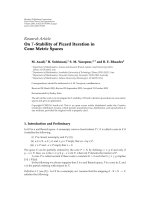
4.1. Influence of intercell interference
Since the complexity of cancellation techniques depends di-
rectly on the number of paths or signals to be canceled, we in-
vestigate the influence of the neighboring signals to the over-
all interfering signal. Figure 7 shows the received C/I ratio at
the mobile terminal for different locations within the cellular
setup for a varying number of interfering cells. We assume
that the MT moves along a straight line between the cell cen-
ter and the outer part of the desired cell centered between
00.20.40.60.811.21.41.6
Distance
−20
−10
0
10
20
30
40
C/I (dB)
1 interfering cell
2 interfering cells
3 interfering cells
4 interfering cells
6 interfering cells
Figure 7: Influence of varying number of interfering cells on the
C/I ratios at different MT positions.
two interfering BSs (α = 30
◦

). At the position d
0
= 1.0, the
MT receives the same signal power from the three closest BSs.
For these simulations, the order of interfering BSs are chosen
by their decreasing distance to the MT. The closest interfer-
ing BS is the first and an SNR of 10 dB is given within all
cells. Since the spreading combines the signals and all avail-
able subcarriers are allocated, there is no difference in the C/I
ratio by varying the system load [26].
The simulation results for one interfering BS show at
d
0
= 1.0 the expected C/I ratio of about 0 dB because both
signals are received with the same power at this location. By
increasing the number of interfering BSs a degradation of the
C/I ratio over all MT positions is given. In the outer regions
of the desired cell (d
0
≥ 0.8) there is no influence on the C/I
ratio for more than two interfering BSs. In the inner part of
the desired cell a small influence of the number of interfering
cells is visible because the MT is nearly equidistant to all sur-
rounding BSs. These results show that the main contribution
of the intercell interference in a cellular MC-CDMA system
is generated by the two closest interfering BSs. Therefore, it is
appropriate and sufficient to take into account only the two
strongest interfering signals for ICIC techniques.
4.2. Impact of hard ICIC
In the following, we verify the results in [18] by using the pro-

posed hard ICIC concepts as described in Section 3.1. These
hard ICIC techniques do not take into account the possible
available signal powers for the equalization process. Figure 8
presents the bit-error rate (BER) performance versus the C/I
ratio. The simulations are carried out with an SNR of 10 dB
and within a two-cell environment where each cell is half
loaded. Therefore, the low C/I values represent the outer part
of the desired cell, C/I
= 0 dB is the cell border, and positive
C/I values are given in the inner cell area.
Simon Plass 7
−10 −50 5 10
C/I (dB)
1e
−04
1e
−03
1e
−02
1e
−01
BER
No ICIC, w/o signal power
Direct hard ICIC, w/o signal power
Indirect hard ICIC, w/o signal power
Mean hard ICIC, w/o signal power
Figure 8: Performance of half-loaded system with different hard
ICIC concepts in the cell border area with an SNR of 10 dB, without
signal power knowledge.
All three hard ICIC concepts can increase the BER per-

formance for low C/I values and at the cell border compared
to the non-ICIC performance. The combination of D-ICIC
and I-ICIC, namely, M-ICIC, can benefit from their perfor-
mance behavior and provides the best performance. Only for
C/I
≤−5 dB, M-ICIC performs worse than D-ICIC because
the first component in the I-ICIC generates wrong estimates
of the recovered signal. This is caused by the weak desired
signal and the hard decided output. Since the decoding and
re-encoding process is not used in the hard ICIC concept, the
performances of the D-ICIC and I-ICIC suffer from wrong
recovered signals in the reconstruction process for high C/I
values. This should be avoided by the soft ICIC concept.
Figure 9 shows the performance gains of the different
combinations for hard ICIC with the proposed knowledge of
the received signal powers. Since the D-ICIC tries to remove
only the interfering signal, it cannot profit from both signal
powers and does not outperform the I-ICIC in contrast to
Figure 8 and [18]. Only for high intercell interference sce-
narios the D-ICIC reconstructs and removes the interfering
signal better than I-ICIC. There is no performances differ-
ence between the I-ICIC and M-ICIC for C/I
≥−5dB.Only
for larger intercell interference the M-ICIC benefits from the
parallel D-ICIC for interfering cell m
= 1 (cf. Figure 4(b)).
But the inner I-ICIC still causes errors and the pure D-ICIC
outperforms the M-ICIC.
By comparing Figures 8 and 9,weseeaperformancedif-
ference of the reference curves without an applied hard ICIC

concept due to the knowledge of the interfering signal power.
There is also a large performance gain for the hard ICIC con-
cepts with the additional information of this power. In terms
of the C/I ratio, the M-ICIC or I-ICIC can gain at the cell
border about 2.5 dB with the additional power information
compared to the M-ICIC without power knowledge.
−10 −50 5 1015
C/I (dB)
1e
−04
1e
−03
1e
−02
1e
−01
BER
No cancelation
DPIC
IdPIC
MPIC
Figure 9: Performance of half-loaded system with different hard
ICIC concepts in the cell border area with an SNR of 10 dB, with
signal power knowledge.
4.3. Impact of soft ICIC
The influence to the performance within a cellular MC-
CDMA system by applying a soft ICIC concept is shown in
the following. It is possible to use the extrinsic information
(cf. (14)) as a degree of reliability for the iterative process
of the signal reconstruction. For the soft ICIC the mean of

the absolute extrinsic information L
E
Decod
over all desired bits
within one OFDM frame is taken to calculate a reliability in-
formation of the decoded signal in the jth iteration following
the definition of soft bits (cf. (7)) by
λ
j
= tanh

1
N
N

n=0


L
E
Decod


/2

, (16)
where N represents the total number of desired bits. Since the
absolute value of L
E
Decod

is taken, the range of λ
j
is now from
[0, 1]. The lower λ
j
the lower is the reliability of a correct
reconstruction of the signal and vice versa. The difference
Δλ
j+1,j
= λ
j+1
−λ
j
(17)
represents the reliability change between the iterations. The
a posteriori knowledge L(c
| q) (cf. (6)) is not taken into
account in this paper which would give a measure of the re-
sulting BER in the final decoding step [27].
A whole tier of cells, that is, 6 interfering cells, around
the desired cell are assumed for the following investigations.
The reliability information λ
j
of the desired signal is sim-
ulated for positions of the mobile terminal in the range of
d
0
= [0.4, 1.4] around the desired BS. The SNR is set to 5 dB
and the system is half loaded. Figure 10(a) shows λ
1

depend-
ing on the position for the first iteration of the soft ICIC in a
three-dimensional illustration. It can be seen that in the in-
ner part of the cell, (d
0
≤ 0.6) λ
1
is mostly 1.0. Therefore,
the desired signal should be detected appropriately in this re-
gion. For the outer parts (d
0
> 0.6) there is a large degra-
dation of the reliability for the decoding process. Differences
8 EURASIP Journal on Wireless Communications and Networking
2
1
0
−1
−2
y-coordinate
10
−6
10
−4
10
−2
10
0
λ
1

−2
−1
0
1
2
x-coordinate
(a) 3D presentation of first iteration
−2 −1.5 −1 −0.50 0.511.52
x-coordinate
−2
−1.5
−1
−0.5
0
0.5
1
1.5
2
y-coordinate
0.1
0.2
0.3
0.4
0.5
0.6
0.7
0.8
0.9
1
λ

1
(b) 2D presentation of first iteration
2
1
0
−1
−2
y-coordinate
10
−6
10
−4
10
−2
10
0
λ
2
−2
−1
0
1
2
x-coordinate
(c) 3D presentation of second iteration
−2 −1.5 −1 −0.50 0.511.52
x-coordinate
−2
−1.5
−1

−0.5
0
0.5
1
1.5
2
y-coordinate
0.1
0.2
0.3
0.4
0.5
0.6
0.7
0.8
0.9
1
λ
2
(d) 2D presentation of second iteration
Figure 10: Resulting values of λ
j
for the desired signal within the coverage of the desired base station depending on the position of the
mobile terminal (base stations have rectangular markers) in two- and three-dimensional representations.
between the mobile terminal position are also visible, for ex-
ample, the mobile terminal experiences one strong interfer-
ing BS ((x, y)
= (−1.4, 0)) or the mobile terminal is located
between two weaker interfering BSs ((x, y)
= (−1.2, −0.7)).

The distribution of λ
2
for the second iteration is shown in
Figure 10(c). Already the second iteration can increase λ
2
over the whole area for this scenario compared to λ
1
.Evenin
the cell border area, (d
0
= [0.8, 1.2]) λ
2
achieves values close
to one. Therefore, this second iteration broadens the area for
successful detection of the desired signal. Another represen-
tation of λ
j
within the cellular environment is given in Fig-
ures 10(b) and10(d) for one and two iterations, respectively.
The positions of the involved BSs are given by the rectangu-
lar marks. These plots show more precisely that in the first
iteration the more reliable λ
1
values are limited to d
0
< 1.0.
For the second iteration reliable, λ
2
values stretch already to
d

0
≤ 1.2.
Due to the large simulation complexity of the whole cel-
lular environment and its reproduction, we also provide the
difference Δλ
2,1
in the three dimensional plot of Figure 11.
It is clearly visible that the rim area gains in reliability for
the decoding process for the second iteration. There are cor-
ridors without an increase of λ
2
due to the constellation of
the cellular environment. Since the signal strength of the two
closest interfering cells in these corridors (e.g., α
= 30
◦
)do
not differ significantly, the soft ICIC process cannot improve
the already good λ
1
values in the second iteration. If only
one BS is the major interferer (e.g., α
= 0
◦
) and the signal
strength between the desired and main interferer differs, the
soft ICIC can detect both signals in the second iteration more
precisely.
The distribution of λ
j

depends directly on the chosen
scenario. Figure 12 presents different SNR scenarios within
a one-tier cellular environment. We investigate λ
j
for the
desired and the two closest interfering signals where the
mobile terminal is located close to the cell border with al-
most the same distance to all these three BSs, that is, d
0
=
0.9, α = 30
◦
,or(x, y) = (0.78, 0.45). Due to the previous re-
sults in Section 4.1, the two closest interfering cells are taken
into account for the soft ICIC process. Furthermore, we as-
sume a single-user case within all cells. For low SNR values
(SNR
≤ 0 dB), low and constant values of λ
j
are given over
all iterations. If the SNR is larger than 2 dB, λ
j
increases for
higher number of iterations. In the case of SNR
= 8 dB, there
Simon Plass 9
2
1
0
−1

−2
y-coordinate
0
0.2
0.4
Δλ
2,1
−2
−1
0
1
2
x-coordinate
Figure 11: Difference Δλ
2,1
= λ
2
−λ
1
of the reliability information
between the first and second iterations of the soft ICIC process.
01234
Iteration
0
0.25
0.5
0.75
1
λ
j

Desired cell
First interfering cell
Second interfering cell
−2dB
0dB
2dB
4dB
8dB
SNR
Figure 12: Reliability of decoding process of recovering the signals
of different cells close to the cell border for several iterations at vary-
ing SNR scenarios.
exists a large step between the first and second iteration but
the following iterations do not increase λ
j
for j>2anymore.
Due to the small power differences of the three received sig-
nal (d
0
= 0.9), the reliability information λ
j
varies for the de-
tected signals. It is obvious that a higher SNR provides better
detection possibilities than low SNR scenarios for the desired
signal.
The same simulation setup is chosen for Figure 13 ex-
cept that this single-user scenario is directly located at the
cell border (d
0
= 1.0, α = 30

◦
). The performance regarding
the BER versus SNR is given. As an upper bound of the sys-
tem, the performance with no ICIC is illustrated. The lower
bound is represented by the single-user performance with-
out any intercell interference. Already the first iteration in-
creases the performance for SNR > 2dB. The second itera-
tion can increase the performance significantly which con-
−20 2 4 6 8
SNR (dB)
1e
−04
1e
−03
1e
−02
1e
−01
BER
Indirect hard ICIC
No ICIC at cell border
Direct hard ICIC
Mean hard ICIC
Soft ICIC, 1 iteration
Soft ICIC, 2 iterations
Soft ICIC, 3 iterations
Soft ICIC, 4 iterations
No inter-cell interference,
single user
Figure 13: Performance of the soft ICIC for the single-user case at

the cell border for different SNR values.
firms the characteristics of the λ
j
values in Figure 12.Even
the single-user bound can be almost reached within 2 itera-
tions for higher SNRs. With 4 iterations it is possible to reach
the single-user bound, and therefore, the intercell interfer-
ence is removed.
For comparison we included the performance curves of
the hard ICIC concepts in Figure 13. Since no decoding is
taken into account in this cancellation technique, the perfor-
mance does not reach the first iteration performance of the
soft ICIC. Still the M-ICIC and D-ICIC can improve the per-
formance significantly compared to no applied ICIC. In con-
trast to a two-cell scenario (cf. Figure 9), the I-ICIC cannot
handle the intercell interference of several interfering cells
appropriately, and therefore, there exists a large performance
loss.
The performance in the cell border area for the soft ICIC
is presented in Figure 14. The SNR is set to 10 dB and the
system is half loaded in all seven cells. The desired and the
two closest interfering cells are chosen to be processed in the
soft ICIC. The mobile terminal moves along a straight line
from d
0
= 0.6tod
0
= 1.6withα = 30
◦
. The performance

without any applied ICIC technique is represented by the
dotted line. For this scenario the first iteration cannot cancel
out the intercell interference. Therefore, the hard ICIC con-
cepts also fail for this scenario, represented by the M-ICIC
performance. The second iteration of soft ICIC can achieve
a small performance improvement. The so-called turbo cliff
is reached with the third iteration and large performance
gains can be achieved. A fourth iteration yields no apprecia-
ble improvement. All performance curves merge to the non-
ICIC curve if they reach the intercell interference free case
(d
0
< 0.8). Directly at the cell border (d
0
= 1.0) all processed
signals are received with the same power, and therefore, the
signals are at most difficult to separate and the soft ICIC per-
formance is worst at this point. Due to the different received
10 EURASIP Journal on Wireless Communications and Networking
0.60.81 1.21.41.6
Distance
1e
−04
1e
−03
1e
−02
1e −01
BER
w/o soft ICIC

Mean hard ICIC
Soft ICIC, 1 iteration
Soft ICIC, 2 iterations
Soft ICIC, 3 iterations
Soft ICIC, 4 iterations
Figure 14: Performance of a half-loaded system with soft ICIC in
the cell border area with an SNR of 10 dB.
signal powers, the soft ICIC can maximize the performance
at d
0
= 1.2. This performance is similar to the almost inter-
cell interference free case at d
0
= 0.8. For larger distances to
the desired BS (d
0
> 1.2), the performance degrades because
the desired signal becomes weak and the final decoding step
for the desired signal can fail.
We can conclude from these investigations that the less
complex hard ICIC concepts can be beneficial in scenarios
where the impinging signals can be well distinguished. This
correlates directly to the behavior of the decoding capabil-
ity of the first iteration in the soft ICIC. The more complex
soft ICIC technique is more robust to different scenarios and
can improve the performance significantly by using several
iterations. Due to the larger complexity of the soft ICIC, this
technique can be applied at receivers with the available pro-
cessing capabilities.
5. CONCLUSIONS

In this paper, we have described and investigated sev-
eral approaches of intercell interference cancellation (ICIC)
schemes in a cellular MC-CDMA downlink environment.
The hard ICIC takes into account the hard decided output
of the demodulator and with the proposed use of the signal
power information the overall performance benefits. A more
sophisticated approach is based on the use of the soft out-
puts of the decoder to reconstruct the signals for cancellation.
Both schemes can improve significantly the performance in
the severe cell border area. Performance results show that the
soft ICIC approaches the single-user bounds without inter-
cell interference, and therefore, the interference of the cellu-
lar environment can be almost eliminated. The extrinsic in-
formation of the decoding process can give a reliability infor-
mation about the successful decoding process, and therefore,
the behavior of the soft ICIC for different scenarios can be
described and analyzed. The profit of the soft ICIC depends
directly on the given scenarios and the used number of itera-
tions.
REFERENCES
[1] IST-4-027756 WINNER Project, />[2] J. A. C. Bingham, “Multicarrier modulation for data transmis-
sion: an idea whose time has come,” IEEE Communications
Magazine, vol. 28, no. 5, pp. 5–14, 1990.
[3] Z. Wang and G. B. Giannakis, “Wireless multicarrier commu-
nications: where Fourier meets Shannon,” IEEE Signal Process-
ing Magazine, vol. 17, no. 3, pp. 29–48, 2000.
[4] K. Fazel and L. Papke, “On the performance of convo-
lutionally-coded CDMA/OFDM for mobile communications
systems,” in Proceedings of the IEEE International Sympo-
sium on Personal, Indoor and Mobile Radio Communications

(PIMRC ’93), pp. 468–472, Yokohama, Japan, September
1993.
[5] N. Yee, J P. Linnartz, and G. Fettweis, “Multi-carrier CDMA
for indoor wireless radio networks,” in Proceedings of the IEEE
International Symposium on Personal, Indoor and Mobile Ra-
dio Communications (PIMRC ’93), pp. 109–113, Yokohama,
Japan, September 1993.
[6] S. Weinstein and P. Ebert, “Data transmission by frequency-
division multiplexing using the discrete Fourier transform,”
IEEE Transactions on Communications,vol.19,no.5,part1,
pp. 628–634, 1971.
[7] K. Fazel and S. Kaiser, Multi-Carrier and Spread Spectrum Sys-
tems, John Wiley & Sons, New York, NY, USA, 2003.
[8] G. Auer, S. Sand, A. Dammann, and S. Kaiser, “Analysis of cel-
lular interference for MC-CDMA and its impact on channel
estimation,” European Transactions on Telecommunications,
vol. 15, no. 3, pp. 173–184, 2004.
[9] S. Plass, S. Sand, and G. Auer, “Modeling and analysis of a cel-
lular MC-CDMA downlink system,” in Proceedings of the 15th
IEEE International Symposium on Personal, Indoor and Mo-
bile Radio Communications (PIMRC ’04), vol. 1, pp. 160–164,
Barcelona, Spain, September 2004.
[10] X. G. Doukopoulos and R. Legouable, “Impact of the inter-
cell interference in DL MC-CDMA systems,” in Proceedings
of the 5th International Workshop on Multi-Carrier Spread-
Spectrum (MC-SS ’05), pp. 101–109, Oberpfaffenhofen, Ger-
many, September 2005.
[11] S. Plass, X. G. Doukopoulos, and R. Legouable, “On MC-
CDMA link-level inter-cell interference,” in Proceedings of the
65th IEEE Vehicular Technology Conference (VTC ’07),pp.

2656–2660, Dublin, Ireland, April 2007.
[12] F. Bauer, E. Hemming, W. Wilhelm, and M. Darianian, “Inter-
cell interference investigation of MC-CDMA,” in Proceedings
of the 61st IEEE Vehicular Technology Conference (VTC ’05),
vol. 5, pp. 3048–3052, Stockholm, Sweden, May-June 2005.
[13] S. Plass, “Hybrid partitioned cellular downlink structure for
MC-CDMA and OFDMA,” Electronics Letters, vol. 42, no. 4,
pp. 226–228, 2006.
[14] S. Plass and A. Dammann, “On the error performance of sec-
torizedcellularsystemsforMC-CDMAandOFDMA,”inPro-
ceedings of the 16th IEEE International Symposium on Personal,
Indoor and Mobile Radio Communications (PIMRC ’05), vol. 1,
pp. 257–261, Berlin, Germany, September 2005.
[15] M. K. Karakayali, G. J. Foschini, and R. A. Valenzuela, “Net-
work coordination for spectrally efficient communications in
cellular systems,” IEEE Wireless Communications,vol.13,no.4,
pp. 56–61, 2006.
Simon Plass 11
[16] I. Katzela and M. Naghshineh, “Channel assignment schemes
for cellular mobile telecommunication systems: a comprehen-
sive survey,” IEEE Personal Communications,vol.3,no.3,pp.
10–31, 1996.
[17] N. Feng, S C. Mau, and N. B. Mandayam, “Pricing and power
control for joint network-centric and user-centric radio re-
source management,” IEEE Transactions on Communications,
vol. 52, no. 9, pp. 1547–1557, 2004.
[18] X. G. Doukopoulos and R. Legouable, “Intercell interference
cancellation for MC-CDMA systems,” in Proceedings of the
65th IEEE Vehicular Technology Conference (VTC ’07),pp.
1612–1616, Dublin, Ireland, April 2007.

[19] S. Kaiser and J. Hagenauer, “Multi-carrier CDMA with it-
erative decoding and soft-interference cancellation,” in Pro-
ceedings of the IEEE Global Telecommunications Conference
(GLOBECOM ’97), vol. 1, pp. 6–10, Phoenix, Ariz, USA,
November 1997.
[20] M. Chacun, M. H
´
elard, and R. Legouable, “Iterative intercell
interference cancellation for DL MC-CDMA systems,” in Pro-
ceedings of the 6th International Workshop on Multi-Carrier
Spread Spectrum, S. Plass, A. Dammann, S. Kaiser, and K.
Fazel, Eds., vol. 1, pp. 277–286, Springer, Herrsching, Ger-
many, May 2007.
[21] S. Plass, “Investigations on soft inter-cell interference cancella-
tion in OFDM-CDM systems,” in Proceedings of the 12th Inter-
national OFDM Workshop (InOWo ’07),Hamburg,Germany,
August 2007.
[22] J. Hagenauer, E. Offer, and L. Papke, “Iterative decoding of bi-
nary block and convolutional codes,” IEEE Transactions on In-
formation Theory, vol. 42, no. 2, pp. 429–445, 1996.
[23] P. Robertson, E. Villebrun, and P. Hoeher, “A comparison of
optimal and sub-optimal MAP decoding algorithms operat-
ing in the log domain,” in Proceedings of the IEEE International
Conference on Communications (ICC ’95), vol. 2, pp. 1009–
1013, Seattle, Wash, USA, June 1995.
[24] P.A.Hoeher,P.Robertson,E.Offer, and T. Woerz, “The soft-
output principle reminiscences and new developments,” Euro-
pean Transactions on Telecommunications, 2007.
[25] G. D. Ott and A. Plitkins, “Urban path-loss characteristics at
820 MHz,” IEEE Transactions on Vehicular Technology, vol. 27,

no. 4, pp. 189–197, 1978.
[26] S. Plass, A. Dammann, and S. Kaiser, “Error performance for
MC-CDMA and OFDMA in a downlink multi-cell scenario,”
in Proceedings of the 14th IST Mobile & Wireless Communica-
tions Summit (IST Summit ’05), Dresden, Germany, June 2005.
[27] S. ten Brink, “Convergence behavior of iteratively decoded
parallel concatenated codes,” IEEE Transactions on Communi-
cations, vol. 49, no. 10, pp. 1727–1737, 2001.