Báo cáo hóa học: " Research Article Dimensioning Method for Conversational Video Applications in Wireless Convergent Networks" docx

Hindawi Publishing Corporation
EURASIP Journal on Wireless Communications and Networking
Volume 2008, Article ID 328089, 14 pages
doi:10.1155/2008/328089
Research Article
Dimensioning Method for Conversational Video
Applications in Wireless Convergent Networks
Alfonso Fernandez-Duran,
1
Raquel Perez Leal,
1
and Jos
´
e I. Alonso
2
1
Alcatel-Lucent Spain, Ramirez de Prado 5, 28045 Madrid, Spain
2
Escuela Tecnica Superior de Ingenieros de Telecomunicaci
´
on, Universidad Polit
´
ecnica de Madrid,
Ciudad Universitaria, 28040 Madrid, Spain
Correspondence should be addressed to Alfonso Fernandez-Duran,
Received 1 March 2007; Revised 19 June 2007; Accepted 22 October 2007
Recommended by Kameswara Rao Namuduri
New convergent services are becoming possible, thanks to the expansion of IP networks based on the availability of innovative
advanced coding formats such as H.264, which reduce network bandwidth requirements providing good video quality, and the
rapid growth in the supply of dual-mode WiFi cellular terminals. This paper provides, first, a comprehensive subject overview as
several technologies are involved, such as medium access protocol in IEEE802.11, H.264 advanced video coding standards, and

conversational application characterization and recommendations. Second, the paper presents a new and simple dimensioning
model of conversational video over wireless LAN. WLAN is addressed under the optimal network throughput and the perspective
of video quality. The maximum number of simultaneous users resulting from throughput is limited by the collisions taking place
in the shared medium with the statistical contention protocol. The video quality is conditioned by the packet loss in the contention
protocol. Both approaches are analyzed within the scope of the advanced video codecs used in conversational video over IP, to con-
clude that conversational video dimensioning based on network throughput is not enough to ensure a satisfactory user experience,
and video quality has to be taken also into account. Finally, the proposed model has been applied to a real-office scenario.
Copyright © 2008 Alfonso Fernandez-Duran et al. This is an open access article distributed under the Creative Commons
Attribution License, which permits unrestricted use, distribution, and reproduction in any medium, provided the original work is
properly cited.
1. INTRODUCTION
A large number of technological changes are today impact-
ing on communication networks which are encouraging the
introduction of new end-user services. New convergent ser-
vices are becoming possible, thanks to the expansion of IP-
based networks, the availability of innovative advanced cod-
ing formats such as H.264, which reduce network bandwidth
requirements providing good video quality, and the rapid
growth in the supply of dual-mode WiFi cellular terminals.
These services are ranging from the pure voice, based on un-
licensed mobile access (UMA) or voice call continuity (VCC)
standards, to multimedia including mobile TV and conver-
sational video communications. The new services are being
deployed in both corporate and residential environments.
In the corporate environments, conferencing and collabora-
tion systems could take advantage of the bandwidth available
in the private wireless networks to share presentation mate-
rial or convey video conferences efficiently at relatively low
communication costs. In the residential segment, mobile TV
and IP conversational video communications are envisaged

as key services in both mobile and IP multimedia subsystem
(IMS) contexts. The success of these scenarios will depend
on the quality achievable with the service, once a user makes
ahandoff from one network to the other (vertical handoff)
and stays in the wireless domain. Video communications are
usually a relatively high wireless resource-demanding service,
because of the amounts of information and the real-time re-
quirements. Services of a broadcast nature usually go down-
link in the wireless network, and therefore contention and
collision have a reduced effect on the network performance
and capacity, while conversational video goes in both direc-
tions, suffering from the statistical behavior of the wireless
contention protocol. The wireless network performance will
depend on the particular video and audio settings used for
the communications, and therefore the network will need to
be designed and dimensioned accordingly to ensure a satis-
factory user experience.
2 EURASIP Journal on Wireless Communications and Networking
Video transmission over WLAN has been analyzed un-
der different perspectives. An analysis of different load con-
ditions using IEEE802.11 is presented in [1]; the study makes
an assessment of the video capacity by measuring capacity in
a reference testbed, but the main focus is on video stream-
ing not on bidirectional conversational video. Although no
dimensioning rules are proposed, it is interesting to men-
tion that the measurements shown mix both contention
protocol and radio channel conditions. The implications of
video transmission over wireless and mobile networks are
described in [2]. Although dimensioning is not targeted, the
paper discusses effects of frame slicing on different numbers

of packets per frame commonly used in wireless networks.
The study shows that a rather low slicing in the order of 6 to
10 packets per frame is a good approach for the packet error
concealment. However, it is not directly applicable to con-
versational video over wireless networks, since the resulting
packet size could be so small that the radio protocol efficiency
is severely affected. Performance and quality in terms of peak
signal-to-noise ratio (PSNR) under radio propagation con-
ditions are shown in [3], and a technique to improve the per-
formance under limited coverage conditions is proposed, but
capacity-limited conditions necessary for dimensioning are
not analyzed. A discussion on the packet sizes and the impli-
cations in the PSNR is presented in [4]. The results shown
are based only on simulations, and no model is proposed to
predict the system performance.
The performance of conversational video over wireless
networks, to be used for network dimensioning purposes,
has to be analyzed under the radio access protocol perspec-
tive to evaluate the implications of the wireless network on
the conversational video. The present study is based on the
analysis of the effects of the medium access protocol used in
IEEE802.11 on the video performance. In a first step, perfor-
mance is analyzed by considering the protocol throughput
as a consequence of contention and collisions. In a second
step, a video quality indicator based on effective frame rate is
used to assess the actual video performance beyond the pro-
tocol indicator, so as to arrive at more realistic dimension-
ing figures. In the present study, the availability of standard-
ized (IEEE802.11e) techniques is assumed for trafficpriori-
tization. The standard reference framework for IP network

impairment evaluation is G.1050, and H.264 is assumed for
service profiles, both from ITU-T [5, 6].
The following sections introduce the framework for con-
versational video applications, a new and simple model of
conversational video over wireless LAN dimensioning, and
show that different results are achieved using throughput and
video quality approaches. Both discrepant results could be
conciliated for proper network dimensioning, as it is also
shown in a real-office scenario.
2. CONVERSATIONAL VIDEO APPLICATIONS
Today’s communication networks are greatly affected by a
number of technological changes, resulting in the develop-
ment of new and innovative end-user services.
One of the key elements for these new applications is
video services that impact on the appearance of new multi-
media services. Voice services are complemented with video
and text (instant messaging and videoconference, etc.) ser-
vices; services can be combined and end-users can change
from one type of service to another. Likewise, multiparty
communication is becoming more and more popular. Ser-
vices are being offered across a multitude of network types.
Examples are multimedia conferences and collaborative ap-
plications that are now enhanced to support nomadic (trav-
eling employees with handheld terminals) and IP access
(workers with an SIP client on their PC and WLAN access).
On the other hand, new devices are being introduced to en-
able end-users to use a single device to access multiple net-
works. Examples include the dual-mode phones, that can
access mobile networks or fixed networks, or handheld de-
vices which support fixed-mobile convergence and conver-

sational video applications [7, 8]. As a consequence of the
evolution of the technologies and applications stated in the
previous paragraphs, a new analysis of conversational video
applications in wireless convergent networks is required. To
do that, ITU-T Rec. H.264
| ISO/IEC 14496-10 and H.264
advanced coding techniques have been considered as a video
coding format. Moreover, ITU-T G.1050 recommendations
have been taken into account as a reference framework for
the evaluation of an IP wireless network section in terms of
delay and random packet loss impact.
2.1. ITU-T G.1050 model considerations
ITU-T G.1050 recommendation [5]specifiesanIPnetwork
model and scenarios for evaluating and comparing commu-
nication equipment connected over a converged wide-area
network. This recommendation describes services’ test pro-
files and applications, and it is scenario-based. In order to
apply it to conversational video applications conveyed over
wireless networks, the following services’ profiles and end-
to-end impairment ranges should be taken into account as a
reference framework.
The contribution to delay (one-way latency) and random
packet loss of the wireless LAN section, analyzed in this pa-
per, should be compatible with the corresponding end-to-
end impairment detailed in Tab le 1 . This should be a bound-
ary condition, in a first step, towards the analytical results.
On the other hand, taking into account the kind of ap-
plications proposed, that is, multivideo conference, fixed-
mobile convergent video applications over a single terminal,
and so forth, the typical scenario location combination will

be business-to-business. However, business-to-home and
home-to-business scenarios should be also considered in the
case of teleworking. Even more new scenarios, not included
in the recommendation, such as business-to-public areas and
vice versa (i.e., airport and hotels) in the case of nomadic
use, could take place. End-user terminals will be PCs and/or
handheld terminals with video capabilities.
2.2. H.264 profiles and levels to be used
H.264 “represents an evolution of the existing video coding
standards (H.261, H.262, and H.263) and it was developed
in response to the growing need for higher compression of
Alfonso Fernandez-Duran et al. 3
Table 1: Service test profiles and impairment ranges.
Service test profile Application (examples)
One-way latency range
Random packet loss range
(min–max) (ms)
(min–max) (%)
Profile A: well-managed
IP network
High-quality video and VoIP, conversa-
tional video (real-time applications, loss-
sensitive, jitter-sensitive, high interaction)
20–100 (regional)
90–300 (intercontinental)
0–0.05
Profile B:partially
managed IP network
VoIP, conversational video (real-time ap-
plications, jitter-sensitive, interactive)

50–100 (regional) 90–400
(intercontinental)
0–2
moving pictures for various applications such as videocon-
ferencing, digital storage media, television broadcasting, In-
ternet streaming, and communication” [6].
The H.264 defines a limited subset of syntax called “pro-
files” and “levels” in order to facilitate video data interchange
between different applications. A “profile” specifies a set of
coding tools or algorithms that can be used in generating a
conforming bit stream, whereas a “level” places constraints
on certain key parameters of the bit stream. The last recom-
mendation version defines seven profiles (baseline, extended,
main, and four high-profile types) and fifteen “levels” per
“profile.” The same set of “levels” is defined for all “profiles.”
Just as an example, the H.264 standard covers a broad
range of applications for video content including real-time
conversational (RTC) services such as videoconferencing,
videophone, and so forth, multimedia services over packet
networks (MSPNs), remote video surveillance (RVS), and
multimedia mailing (MMM), all of them are very suitable
to be deployed over convergent networks.
In this paper, video applications have focused on baseline
and extended profiles and low rates (64, 128, and 384 Kbps)
corresponding to levels 1, 1.b, and 1.1 of the H.264 standard.
The new capabilities and increased compression efficiency of
H.264/AVC allow for the improvement of the existing appli-
cations and enable new ones. Wiegand et al. remark the low-
latency requirements of conversational services in [9]. On the
other hand, they state that these services follow the baseline

profile as defined in [10]. However, they pointed out the pos-
sibility of evolution to the extended profile for conversational
video applications.
3. THROUGHPUT-BASED CAPACITY IN WLAN
This section describes a simple method to estimate the video
capacity in IEEE802.11 networks by estimating the effect of
collisions on the air interface. This method is based on the
principles described in [11], further developed in [12], and
adapted to voice communications in [13].
3.1. Principles for throughput estimation
In general, a station that is going to transmit a packet will
need to wait for at least a minimum contention window,
following a distributed interframe space (DIFS) period in
which the medium is free. If the medium is detected as busy,
the packet transmission is delayed by a random exponential
backoff time measured in slot times (timing unit). Looking
at the IEEE802.11 family, there are differences in duration for
the same parameter. This set of values is very relevant since it
defines the performance of the network for each of the PHY
standards [13–16].
The first step in the analysis of the protocol, CSMA-CA, is
to determine the time interval in which the packet transmis-
sion is vulnerable to collisions. Looking at the distributed co-
ordination function (DCF) timing scheme based on CSMA-
CA with request-to-send-clear-to-send (RTS-CTS), it ap-
pears that during the time interval of DIFS and an RTS
packet, a collision could take place. This assumption is true
in the case of a hidden node. This hidden node effect is likely
to happen with certain frequency. For example, in an ac-
cess network using directional antennas, most of the nodes

cannot see each other, that is, most of the nodes are hid-
den. If we denote the period in which the protocol is vul-
nerable to collisions as τ, this could be expressed as τ
=
η(t
DIFS
+ t
RTS
+ t
SIFS
)+t
p
,wheret
DIFS
is the duration of DIFS
interval, t
RTS
is the duration of the signaling packet, t
SIFS
is
the duration of short intraframe space (SIFS) interval, t
p
is the propagation time, and η is the proportion of hidden
nodes. The packet transmission has several parts: the packet
transmission itself, made up of the packet duration T,part
of which is the vulnerability period τ, and the waiting inter-
vals part in which no transmission takes place. In the case
of very few hidden nodes, it is possible not to use the RTS-
CTS protocol, but CTS-to-self. The new vulnerability period
could be estimated as τ

= η(t
DIFS
+ t
CTS
+ t
SIFS
+ T)+t
p
. The
relationship between the vulnerability period and the dura-
tion of the packet transmission is α
= τ/T. This value is key
in estimating the network efficiency. Following the notation
introduced in [17], it is possible to obtain the basic expres-
sions that could be developed to obtain the parameters that
influence the video network throughput and the estimated
quality.
3.2. Contention window
The contention window as defined in IEEE802.11 is a mech-
anism with big influence on the network behavior since it has
a significant impact on the collision probability.
Let the probability of collision or contention in a first
transmission attempt be
P
c
=

1 − P
ex


P
CW0
=

1 − e
−gτ

P
CW0
=

1 − e
−αG

P
CW0
,
(1)
where P
CW0
is the probability that another station selects the
same random value for the contention window, P
ex
is the
4 EURASIP Journal on Wireless Communications and Networking
probability of a successful packet transmission, g is the packet
arriving rate in packets/sec, and G is the offered traffic.
Extrapolating to n transmission attempts
P
c

=
n

i=1

1 − e
−αG

i
P
CW(i−1)
,(2)
where P
CW(i)
will be given by
P
CWi
=
N −1
CWi +1
,(3)
with CWi being the maximum duration of the contention
window in the current status according to [17]andN the
number of simultaneous users.
Combining previous equations, the expected value of the
contention window will be given by
CW
= CW
0
+

n

i=1
CWi
CWi +1
(N
−1)(1 −e
−αG
)
2i+1
. (4)
3.3. Throughput estimation
Taking the approach introduced by [11] and further devel-
oped in [12, 13], following the sequence of activity and in-
activity periods, and because the packet streaming process is
memoryless, we can consider the process of busy transmis-
sion duration times

B and B as its average value. Similarly,
we could call

U the process of durations in which transmis-
sions are successful (with average value U), and

I the dura-
tion of waiting times with average I; therefore the process for
the transmission cycles will be

B +


I, and the throughput will
be obtained from
S
=
U
B + I
. (5)
Let us consider first the inactivity period. This duration is
the same as the duration of the interval between the end of a
packet transmission and the beginning of the next one. Since
the packet sequencing is a memoryless process, we could ex-
press
F
I
(x) = prob


I ≤ x

= 1 −prob


I>x

(6)
= 1 −P[No packet sent during x] = 1 − e
−gx
. (7)
This means that “I” has an exponential distribution with
average

I
=
1
g
. (8)
Following [11–13], and introducing the effect of the con-
tention window described above, we obtain
U
= T

1 − P
CW
+ P
CW
e
−gτ

,
B
= T + τ + P
CW

τ −
1 − e
−gτ
g

.
(9)
1000010001001010.10.010.001

Normalized offered traffic
0
10
20
30
40
50
60
70
80
Throughput (%)
Protocol efficiency
802.11b
802.11b + g
802.11g
802.11a
Figure 1: Throughput efficiency in IEEE802.11.
Table 2: Example of vulnerability factors for packet lengths of 1024
bytes in the different variants of the IEEE802.11 standard.
802.11b 802.11b + g 802.11g 802.11a
Vulnerability factor (α) 0.129 0.120 0.123 0.122
Combining the above results, we finally obtain
S
=
U
B + I
=
T

1 − P

CW

1 − e
−gτ

T + τ + P
CW

τ − (1 −e
−gτ
)/g

+1/g
. (10)
To t u rn S into a more manageable format, we can nor-
malize (10) with respect to the duration of the packet trans-
mission period. If G represents the average packet transmis-
sion time measured in packets per packet transmission pe-
riod, that is,
G
= gT, (11)
using the vulnerability factor defined above, we obtain
α
=
τ
T
. (12)
The throughput expression results in the following:
S
=

G

1 − P
CW

1 − e
−αG

1+P
CW
+ G

1+α

1+P
CW

+ P
CW
e
−αG
. (13)
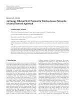
Taking the timing values defined in the standard, the
throughput versus the normalized offered load G for the dif-
ferent values of vulnerability factor in the different variants
of IEEE802.11 is shown in Figure 1.
As can be seen, the relative efficiency in the four func-
tional variants of the standard is practically the same. This is
due to the fact that the resulting vulnerability factor for all of
them is very similar as shown in Ta b le 2 .

If we compare the efficiency of this protocol with the ca-
ble protocols such as Ethernet, we see that the latter are more
efficient. This is because the vulnerability factor resulting in
the radio protocol is larger. While the IEEE802.11 protocol-
reaches maximum throughput at around 70%, as shown in
Alfonso Fernandez-Duran et al. 5
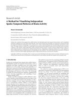
Packet no. 1 Packet no. 2 Packet no. 3 ········· Packet no. N
T
T/G
T
t
Figure 2: Time representation of offered traffic(G), number of si-
multaneous users (N), and expected packet (T)andframe(T
t
)du-
rations.
Figure 1, partially because of the contention window, Ether-
net networks reach 90% in the same packet size (1024 bytes).
It has to be noted that the throughput decreases with the
decrease in the packet size since the relative transmission
time decreases, and then the vulnerability factor increases.
It is therefore evident that the protocol is more efficient with
larger packets than with smaller ones.
3.4. Throughput-based service dimensioning in WLAN
The analysis described so far shows the system’s behavior in
normalized terms, with no relationship to the transport of a
specific service.
The offered traffic G has to be associated with the num-
ber of users to whom a given capacity is offered, in such a
way that the throughput is represented as a function of the

number of users requiring a given type of service.
For a type of service characterized by a bit rate r
b
and an
IP packet size n
b
, we will get an average data frame duration
for the service:
T
t
=
n
b
r
b
. (14)
If we also assume that the packet duration is T, the rela-
tionship between the trafficoffered (G) and the number of
sources (N) will be given by the following expression:
G
=
1
T
t
/NT −1
. (15)
Or in other terms,
N
=
GT

t
T(1 + G)
. (16)
Figure 2 shows a representation of the timing involved to
obtain the relationship between G and N.
As can be seen, the saturation point of the system is
reached for values of N that are very sensitive to the packet
size required by the service, regardless of the total bandwidth
required. This fact is very relevant since it anticipates that the
system performance will be very dependent on the service in-
formation structure apart from its bandwidth requirements.
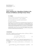
Combining expressions (13)and(15), it is possible to
represent the throughput as a function of the number of si-
multaneous users. Figure 3 shows an example of the behavior
of the IEEE802.11 family of physical layers for given service
bandwidth and packet size.
20100
Simultaneous users
0
10
20
30
40
50
60
70
80
90
Throughput (%)
480-byte packet traffic performance in IEEE802.11

IEEE802.11b
IEEE802.11b + g
IEEE802.11g
IEEE802.11a
Figure 3: Throughput versus number of users for 480-byte packets
in IEEE802.11 variants, for a service of 384 Kbps.
Table 3: Maximum number of users for the variants of IEEE802.11.
802.11b 802.11b + g 802.11g 802.11a
480-byte packets
N
max
3111616
As shown in Figure 3, the throughput reaches a maxi-
mum for a specific value of N depending on the service char-
acteristics. Specifically, the maximum values reached in the
above figure are shown in Ta bl e 3.
It appears to be clear that both the throughput and the
maximum number of users are very sensitive to the packet
size used. As a reference value, 480-byte packets have been
used to determine the maximum system throughput. The
maximum system throughput turns out to be below 80% of
the capacity offered by the physical interface.
As apparent, it is necessary to estimate the maximum
number of simultaneous users that yields the maximum
throughput for a given service configuration. To obtain this
value (N
max
), it is necessary to calculate the maximum of the
expression S(N). Unfortunately, the maximum of S versus N
leads to an expression without an exact analytical solution.

To arrive at an approximate solution, it is necessary to carry
out a polynomial development of one of the terms, which
eventually yields the following expression:
G
max
≈
√
5+4/α −1
α +1
. (17)
Since N is an integer value, we can assume that the ap-
proximated expression matches the exact solution with a rea-
sonable number of terms in the development. The combina-
tion of (16)and(17) produces the following result:
N
max
= Int

T
t

√
5+4/α −1

T

√
5+4/α + α



. (18)
With this expression, we could apply the figures of the
typical multimedia services, that is, data, voice, and video.
6 EURASIP Journal on Wireless Communications and Networking
Table 4: Conversational video service parameters for H.264 at
384 Kbps.
802.11b 802.11b + g 802.11g 802.11a
Phy. capacity
(Mbps)
11 54 54 54
IP packet size (bytes)
240 240 240 240
IP+UDP+RTP
headers (bytes)
40 40 40 40
T(s)
2, 31
·10
−3
6, 73·10
−4
4, 53·10
−4
4, 59.10
−4
Concatenation
1111
T
t
(s)

0,005 0,005 0,005 0,005
α
1, 74
·10
−1
1, 19·10
−1
1, 28·10
−1
1, 26.10
−1
G
max
3,66 4,66 4,45 4,49
N
max
2699
151050
Simultaneous users
0
10
20
30
40
50
60
70
80
90
Throughput (%)

384 Kbps packet video traffic performance in IEEE802.11
IEEE802.11b
IEEE802.11b + g
IEEE802.11g
IEEE802.11a
Figure 4: 384 Kbps conversational video over IP performance with
IEEE802.11e protocol using 240-byte packets.
3.5. Throughput of conversational video
over IP service
Conversational video over IP introduces additional restric-
tions to the system, mainly resulting from the average band-
width required. Since voice and telephony traffic character-
istics are well known, their Poisson process characteristics
match the contention model described in the previous sec-
tions very well. This is still valid even with the introduction
of prioritization mechanisms from IEEE802.11e.
Considering the use of 384 Kbps video codec, the service
will be defined by the parameters shown in Ta bl e 4.
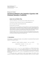
With the service configuration defined as shown in
Ta bl e 3, it results in a behavior as shown in Figure 4.
As it becomes apparent, the differences between the
IEEE802.11 physical layer variants are significant. In addi-
tion, it has to be noted that, depending on the particular
operating conditions, that is, on the maximum capacity of-
fered by the physical layer, the video codec used, video frame
size, and so forth, the results could differ significantly. For
Table 5: Throughput-based video capacity.
Throughput-based video conversations
802.11b 802.11b + g 802.11g 802.11a
64 Kbps 11 36 52 51

128 Kbps 5 19 27 27
384 Kbps 2 6 9 9
1009080706050403020100
Proportion of hidden nodes (%)
10
15
20
25
30
35
Maximum number of users
Protocol and hidden node effects for 128Kbps
conversational video using IEEE802.11g
RTS-CTS
CTS-to-self
Figure 5: Effect of hidden node on the system capacity.
example, Tab le 5 shows the maximum number of simultane-
ous users using 240-byte packets which is a typical expected
packet size in conversational video applications.
3.6. RTS-CTS versus CTS-to-self approach for
conversational video capacity
In the normal use of WLANs, it is possible to select the use
of the RTS-CTS protocol or leave it in the default CTS-to-
self mode. In conditions in which many users share the air
interface, and in conditions in which a hidden node effect
appears, it is reasonable to use the RTS-CTS protocol to en-
sure system performance in terms of delay and capacity. On
the other hand, when few users share the medium, it could
happen that the use of the CTS-to-self mode provides some
improvement. This section compares both protocols belong-

ing to the IEEE802.11, to determine the optimal conditions
of use as a function of the hidden nodes in the network.
According to the definition of the protocol in Section 3,
the protocol performance in terms of throughput is condi-
tioned by the vulnerability time period. The difference be-
tween RTS-CST and CTS-to-self is twofold. On the one hand
RTS-CTS uses extra resources to manage the protocol, but
it has a reduced vulnerability time period, and on the other
hand, CTS-to-self uses fewer network resources, but it has a
longer vulnerability period. Comparing the two approaches,
there is a tradeoff between use of resources and vulnerability
to collisions.
To illustrate the effect of hidden nodes on the system ca-
pacity, the two protocol variants RTS-CTS and CTS-to-self
have been compared, and the results are shown in Figure 5.
Alfonso Fernandez-Duran et al. 7
As the proportion of hidden nodes increases, the prob-
ability of collision also increases regardless of the protocol
scheme selected. In the case of RTS-CTS scheme, mecha-
nisms to maintain the vulnerability time period under cer-
tain limits are available. This is why the reduction in capacity
is in the order of 16%. In the case of CTS-to-self, the vulner-
ability time period is extended to the complete packet, and
that is why it experiences a capacity reduction in the order of
47%. Depending on the particular network conditions and
services, the figures could differ, but in general terms, the use
of RST-CTS protocol appears to be advantageous for services
with moderate number of users.
A simple and approximated approach to estimate the per-
formance in hidden node conditions consists of substituting

α in (18)withα

η,whereη is the estimated proportion of
hidden nodes.
3.7. Influence of conversational video
packaging on the performance
According to the system performance estimation shown in
Section 3.3, the total system capacity and throughput could
depend significantly on the expected packet size used by the
service. Because of the nature of video payload, it cannot be
guaranteed that IP packets are of a given size; nevertheless
the video IP packet sizes correspond to a multimodal distri-
bution in which only certain values are possible. Therefore,
the analysis has to be based on the expected packet size val-
ues. Depending on the profile and the group of video objects
(GoV) scheme selected, the expected packet size delivered
could differ,unlessmeasuresaretakentoensureanaverage
packet size. The larger the packet size used for a given ser-
vices, the higher the throughput and capacity of the system
will be.
Let us take the expected packet size as
E(s)
= S =

k
s
k
P
k
, (19)

where s is the distribution of packet sizes, s
k
are the discrete
values associated to s,andP
k
is the probability of occurrence
of each type of packet sizes.
To illustrate the effect of the packet size on the perfor-
mance, Figure 6 shows how the maximum number of si-
multaneous users could increase the expected payload packet
size.
This behavior follows two principles: the larger the ex-
pected payload packet sizes are, the fewer number of packets
will be needed to maintain the average bit rate, and there-
fore less collision events may occur, and the larger the packet
is, the lower the impact of the necessary headers will be. As a
counterpart, if radio channel conditions suffer from degrada-
tion (increase in the packet error rate), the total video PSNR
could be reduced as described in [4]. In general, the frame
slicing of conversational video will be rather small.
3.8. Audio and video performance interaction
Audio could also play an important role in conversational
video communications. There are two possibilities to con-
450400350300250200150100
Payload packet size (bytes)
0
2
4
6
8

10
12
14
16
Maximum simultaneous users
Influence of packet size on the network
performance for 384 Kbps conversational video
IEEE802.11b + g
IEEE802.11g
Figure 6: Influence of packet size on the system performance.
vey the audio: including the audio as part of the audio and
video payload, taking advantage of packet grouping and syn-
chronization, or taking audio and video streams separately
through the network, making it possible to have a greater
diversity of end-user profiles and devices. Both schemes are
equally used for conversational video calls, but from the wire-
less protocol point of view, the interleaving of audio and
video has advantage of performing close to the case of video
only.
The case of separate audio and video streams is very com-
mon for multiconference environments where user terminals
could have audio only or audio and video capabilities, and all
could take part in the same conference. Many cases of sepa-
rate audio and video flows come from the fact that part of the
communication is conveyed through a network (e.g., audio
through the cellular mobile) and the other part is conveyed
through an IP wireless network (e.g., video part through
IEEE802.11 interface). These conditions are easily experi-
enced using dual-mode cellular wireless terminals. In the
case of using strictly separate audio and video streams, some

extra room has to be allowed to allocate the audio streams
in the network. Fortunately, both audio and video behaviors
are sufficiently linear below the maximum throughput, and
this allows the combination of the two services using simple
proportion rules. For example, if under certain conditions an
IEEE802.11g network can afford 21 G.729 calls or 9 H.264
384 Kbps video calls. However, if we combine separate audio
and video streams, the total audio plus video calls will be in
the order of 6. More information of the voice capacity esti-
mation can be found in [17, 18, 20, 21].
4. VIDEO QUALITY ESTIMATION PRINCIPLES
As described in previous sections, the maximum number
of simultaneous users running conversational video appli-
cations can be estimated from the maximum throughput of
the IEEE802.11 protocol. Moving to a more user-centric ap-
proach, it would be convenient to estimate the conversational
video capacity also based on the video quality. By following
8 EURASIP Journal on Wireless Communications and Networking
this approach, it appears that the maximum number of si-
multaneous users could be different.
The first step is to select a reasonable video quality indi-
cator that relates quality to the wireless network conditions.
The two main potential indicators of the network conditions
are the delay for packet delivery and the packet loss probabil-
ity.
A usual approach to estimate video quality is the peak
signal-to-noise ratio (PSNR), or more recently video qual-
ity rating (VRQ); both are usually estimated from the mean
square error (MSE) of the video frames after the impairments
(e.g., packet loss) with respect to the original video frames

[22, 23]. From these values, there is some correlation to video
mean opinion score (MOS). Unfortunately, the relationship
between packet loss and MSE is not straightforward since not
all packets conveyed through the wireless network have the
same significance. Alternatively, a relatively simpler quality
indicator introduced in [24] is proposed. This indicator is
the effective frame rate that is introduced and discussed in
later sections of this paper.
As packet errors occur in the wireless network, video
frames are affected, making some of them unusable, and
therefore the total frame rate is reduced. Video quality will
be acceptable if the expected frame rate of the video conver-
sationsiskeptabovecertainvalue.
4.1. Delay in conversational video over
IP in wireless networks
A very important characteristic in conversational video com-
munications is the end-to-end delay, since it could have a di-
rect impact on the perceived communication quality, by pro-
ducing buffering or synchronization problems between au-
dio and video in case of separate streams.
To estimate the delay contribution introduced by the
wireless network, let us proceed as in Sections 3.2 and 3.3.
According to (1), the probability of success for a packet trans-
mission is given by the following expression:
P
ex
= e
−gτ
. (20)
The probability of a packet transmission being unsuc-

cessful will be
P
c
= 1 −P
ex
= 1 −e
−gτ
. (21)
Because of the IEEE802.11 operation, we know that in
the case of unsuccessful packet delivery at the first attempt,
the backoff time is increased to the next integer power of
two. This in turn will be the window to generate a random
waiting time before the transmission or retransmission takes
place. Although many retransmissions could take place be-
fore a packet is successfully delivered, there is a dominant in-
fluence on the first retransmission to the total delay. Since
the rest of the packet transmissions are not necessarily in the
same contention window backoff, the nominal delay will be
given by
C
=

b +(N −1)T

P
c
=

b +(N −1)T


1 − e
−gτ

, (22)
1197531
Simultaneous users
0
1
2
3
4
5
6
Delay (ms)
Network delay versus simultaneous video users using H.264 at 384 Kbps
802.11b
802.11b + g
802.11g
802.11a
Figure 7: Video communication delay for the different variants of
IEEE802.11 as a function of the number of simultaneous users.
Table 6: Video transmission delay values in the maximum through-
put conditions for H.264 at 384 Kbps.
802.11b 802.11b + g 802.11g 802.11a
N
max
2699
Expected delay (ms) 1.9 1.3 1.2 1.1
where N is the number of simultaneous voice communica-
tions and b is the backoff time.

The expected value for the duration of a transmission will
be given by the time associated to the successful transmis-
sions and the time associated to the retransmissions. There-
fore the expected delay will be
D
= C + Te
−gτ
=

b +(N −1)T

1 − e
−gτ

+ Te
−gτ
(23)
or
D
=

b +(N −2)T

1 − e
−gτ

+ T. (24)
Combining (11), (12)and(15), (24) can be also ex-
pressed using the service variables as
D

=

b +(N −2)T

1 − e
−α(NT/(T
t
−NT))

+ T. (25)
As can be seen in Figure 7, the delay grows monotoni-
cally with the number of simultaneous video communica-
tions, until the point at which network saturation is reached.
Under these conditions, the delays that are achieved are those
corresponding to the maximum throughput conditions. An
example of these results is shown in Ta bl e 6 .
The delay values shown so far take into account only the
delay introduced by the wireless network in the uplink. To
consider the total delay, it is necessary to introduce the delays
introduced by the voice codecs, the concatenation delay, and
any other delay resulting from the video processing.
The total delay contribution from the wireless network
could be comparatively smaller than the delay resulting from
the rest of the actions taking place in the conversational video
transmission. As an example, it is common that video codecs
introduce delays for frame buffering and video processing. In
the case of 16 frames per second, the delay of a single frame
Alfonso Fernandez-Duran et al. 9
1197531
Users

0
20
40
60
80
100
(%)
802.11b
802.11b + g
802.11g
802.11a
Figure 8: Packet loss probability as a function of the number of
simultaneous users for H.264 at 384 Kbps.
buffering will be 62.5 milliseconds, which is about one order
of magnitude longer than the delay introduced by the wire-
less protocol. As it is detailed in [25], additional processing
delay has to be added to the buffering delay. Therefore, by
comparison, there is no impact on the display deadline vio-
lations caused by the protocol contention or collision. On the
other hand, the contribution of the protocol to the resulting
delay is compatible with the one-way latency expected in Pro-
file B, partially managed IP networks defined in G.1050 [5],
and even in most of the scenarios, it will also be compatible
with Profile A; so the impact on quality should be low.
4.2. Packet loss of conversational video over
IP in wireless networks
The network throughput behavior is not monotonic as
shown in previous sections. This effect is a result of the in-
crease in the number of retransmissions that produces an
avalanche effect. In the case of conversational video over IP,

the maximum number of retransmissions to deliver the same
voice packet should remain limited. According to [4], the in-
crease in the number of transmission attempts from two to
three has a maximum improvement of 2 dB in PSNR, and
further increase has practically no effect on the PSNR. This
in addition avoids an unnecessary increase in delay and jit-
ter. Following this rationale, the maximum number of packet
reattempts could be limited to two, and after that, the packet
is dropped.
If the probability of successful packet transmission is
given by (7) or equivalently by P
= e
−αG
, then the proba-
bility of two consecutive packets being unsuccessful will be
given by
P
pl
=

1 − e
−αG

2
=

1 − e
−α(NT/(T
t
−NT))


2
. (26)
Taking the values shown in previous sections for G and
α, the packet loss probability becomes as shown in Figure 8.
Although packet loss probabilities shown could reach rel-
atively high values, the maximum acceptable limit is around
20%. These values will be used later to estimate their influ-
ence on the resulting video conversation quality.
4.3. Packet loss and radio propagation channel
Although the discussion in the previous sections is mainly
focused on the radio protocol performance, radio propaga-
tion conditions have a decisive impact on the performance of
the conversational video. To illustrate this fact, it is necessary
to understand the behavior of the signal strength. In complex
propagation scenarios, such as indoor ones, small changes in
the spatial separation between wireless access points and ob-
servation points bring about dramatic changes in the signal
amplitude and phase. In typical wireless communication sys-
tems, the signal strength analysis is based on the topologies
of combined scenarios that experience fading, produced by
several causes. Several propagation studies assume that the
fading can be modeled with a random variable following a
lognormal distribution as described in [26–28] in the form
of
f
i
(s) =
1
σ

i
√
2π
e
−(s−μ

i
)
2
/2σ
2
i
, (27)
where
s is the received path attenuation represented in dB, μ

i
is the average signal losses received at the mobile node from
the wireless access point i and could be expressed as
μ

i
= k
1
+ k
2
log (d
i
). (28)
μ


i
represents the propagation losses at the observation point
from the access point (AP), AP i,andd
i
represents the dis-
tances from the observation point to the wireless access point
i. Constants k
1
and k
2
represent frequency-dependent and
fixed attenuation factors and the propagation constant, re-
spectively. Finally σ
i
represents the fading amplitude.
The received signal strength could be similarly expressed
as
μ
i
= P
tx
−

k
1
+ k
2
log


d
i

, (29)
where P
tx
is the transmitted power.
Following this principle for dimensioning purposes,
video packets will be lost in conditions in which the signal
strength falls below a sensitivity threshold s
T
. Therefore the
probability of having a signal strength outage would be
P
T
= P

s>s
T

= 1 −P

s<s
T

= 1 −F

s
T


, (30)
where F is the cumulative distribution function of f ,com-
monly represented as
F
i
(s) =
1
σ
i
√
2π

s
0
e
−(r−μ

i
)
2
/2σ
2
i
dr. (31)
Equation (31) does not provide information on the dura-
tion and occurrence rate of the fading; nevertheless extensive
measurement campaigns have shown that fading tends to oc-
cur in lengthy periods and at a low frequency as described in
[28], rather than short isolated and frequent events. On the
10 EURASIP Journal on Wireless Communications and Networking

−66−68−70−72−74−76−78−80
Signal strength (dBm)
0
0.01
0.02
0.03
0.04
0.05
0.06
0.07
0.08
0.09
0.1
−88 dBm
−90 dBm
Figure 9: Packet error probability as a function of the signal
strength for 6 dB lognormal fading.
other hand, since conversational video packets are of rela-
tively short duration (e.g., 5 milliseconds), the probability of
outage as provided in (30) could be taken as an estimate of
the packet loss probability for a set of channel conditions.
In selecting a set of typical working conditions, it is pos-
sible to estimate the probability of packet errors due to the
fading. For instance, selecting σ
= 6 dB lognormal fading
and sensitivity thresholds of
−88 dBm and −90 dBm, the re-
sults are shown in Figure 9. The signal strength shown on the
horizontal axis is the average power estimated using a propa-
gation model like the one described in ITU-R recommenda-

tion P.1238-3, once the average power is obtained. It is then
possible to estimate the link performance in terms of packet
losses. In the case of network deployment with good cover-
age (
−76 dBm to −73 dBm average), the packet loss is kept
below 1%.
5. CONVERSATIONAL VIDEO CAPACITY OVER
WIRELESS LAN BASED ON QUALITY
As mentioned in Section 4, a good approach to estimate the
video quality is based on evaluating the frame rate drop due
to the impact of packet losses on the video frame integrity.
The sources of packet losses are on one hand the con-
tention protocol, and on the other hand the losses caused
by the radio channel conditions. For specific scenarios, both
should be taken into account. Since both processes are statis-
tically independent, the total packet loss could be obtained as
the addition of both. Nevertheless, to analyze the effect of the
contention protocol, it is assumed that the radio propagation
conditions are sufficiently good to consider the contention
protocol as the dominant effect.
The consequence of a packet loss in a generic video se-
quence depends on the particular location of the erroneous
packet in the compressed video sequence. The reason for this
is related to how compressed video is transmitted through
the IP protocol. The plain video source frames are com-
pressed to form a new sequence of compressed video frames.
The new sequence, depending on the H.264 service profile
applied, could be made up of three types of frames: I (Intra)
frames that transport the content of a complete frame with
IPBBPB BP BB PBB PBB

Figure 10: Compressed video frame-type interrelations.
lower compression ratio, P (Predictive) frames that trans-
port basic information on prediction of the next frame based
on movement estimators, and B (Bidirectional) frames that
transport the difference between the preceding and the next
frames. These new frames are grouped in the so-called group
of pictures (GoP) or groups of video objects (GoV) depend-
ing on the standard. The GoV could adopt many forms and
structures, but for our analysis, we assume a typical config-
uration of the form IPBBPBBPBBPBBPBB. This means that
every 16 frames there is an Intra followed by Predictive and
Bidirectional frames. IP video packets are built from pieces
of the aforementioned frame types and delivered to the net-
work. If a packet error has been produced in a packet belong-
ing to an Intra frame, the result is different from the same
error produced in a packet belonging to a Predictive [29]or
Bidirectional frame. A model is proposed in [24]tocharac-
terize the impact of packet losses on the effective frame rate
of the video sequence.
There are some characteristics that are applicable to the
case of conversational video, and in particular to portable
conversational video, and that are not necessarily applicable
to other video services like IPTV or video streaming. The first
important characteristic is the low-speed and low-resolution
formats (CIF or QCIF) that in turn produce a very low num-
ber of packets per frame, especially if protocol efficiency is
taken into account increasing the average packet size (see
Figure 6). In these conditions, a single packet could convey
a substantial part of a video frame. The second important
characteristic comes from the portability and low consump-

tion requirement at the receiving end that in turn requires
a lighter processing load to save battery life. The combina-
tion of the two aforementioned characteristics makes those
packet losses impact greatly on the frame integrity, and con-
cealment becomes very restrictive. In conversational video, it
could be better, for instance, to maintain a clear fixed image
of the other speaker on the screen than to try error compen-
sation at the risk of severe image distortions and artifacts.
Following these characteristics, every time a packet is lost in
a frame, the complete frame becomes unusable, and some ac-
tion could be taken at the decoder end, to mitigate the effect
such as freezing or copying frames, but the effective frame
rate has been reduced, and it has to afford some form of video
quality degradation.
Following the notation in [24], the observed video frame
rate will be f
= f
0
(1−φ), where φ is the frame drop rate and
f
0
is the original frame rate.
Alfonso Fernandez-Duran et al. 11
7531
Simultaneous users
0
2
4
6
8

10
12
14
16
18
Frame rate
Quality degradation for 384 Kbps H.264
conversational video
IEEE802.11b
IEEE802.11b + g
IEEE802.11g
IEEE802.11a
Figure 11: Frame rate as a function of simultaneous users for
384 Kbps H.264 CIF.
In turn, the frame drop rate comes from
φ
=

i
P

f
i

P

F


f

i

, (32)
where “i” denotes the different types of I, P, and B frames,
P( f
i
) is the fraction of bit streams from each type of frames,
and P(
F | f
i
) is the conditional probability of having a packet
loss on a frame of type i. The latter can be estimated by taking
into account the interrelation between frames as shown in
Figure 10.
As a consequence of this, [24] arrives at closed form ex-
pressions for the conditional probabilities as follows:
P

F|@I

=
1 − (1 − p)
S
I
, (33)
P

F



P

= 1 −
(1 − p)
S
I
N
P

1 − (1 − p)
S
P


1 − (1 − p)
S
P
N
P

,
(34)
P

F


B

≤ 1 −

(1 − p)
S
I
+S
P
+S
B
N
P

1 − (1 − p)
S
P


1 − (1 − p)
S
P
N
P

,
(35)
where S
I
, S
P
,andS
B
are the number of packets in the re-

spective frame types and N
P
is the number of P frames. For
simplicity, in this estimation, it is considered that a packet
loss within a frame produces an unusable frame. Although
the assumption is very restrictive, it yields a conservative in-
dicator of quality.
Combining (26)to(35), it is possible to obtain a simple
video quality estimator based on the effective frame rate re-
sulting from the packet losses. In Figures 11–13, the effective
frame rate reduction as the number of simultaneous conver-
sational video users increases is shown, for the cases of H.264
at 384 Kbps CIF format, and 128 Kbps and 64 Kbps QCIF
formats.
From the results above, it is possible to obtain the maxi-
mum number of simultaneous users that ensures a minimum
frame rate, and therefore dimensioning could be related to a
quality estimator. As a quality limit indicator, a frame rate of
2621161161
Simultaneous users
0
2
4
6
8
10
12
14
16
18

Frame rate
Quality degradation for 128 Kbps H.264 QCIF
conversational video
IEEE802.11b
IEEE802.11b + g
IEEE802.11g
IEEE802.11a
Figure 12: Frame rate as a function of simultaneous users for
128 Kbps H.264 QCIF.
464136312621161161
Simultaneous users
0
2
4
6
8
10
12
14
16
18
Frame rate
Quality degradation for 64 Kbps H.264 QCIF
conversational video
IEEE802.11b
IEEE802.11b + g
IEEE802.11g
IEEE802.11a
Figure 13: Frame rate as a function of simultaneous users for
64 Kbps H.264 QCIF.

Table 7: Quality-based conversational video capacity.
Quality-based video conversations
802.11b 802.11b+g 802.11g 802.11a
64 Kbps 7 28 40 39
128 Kbps 3 13 19 19
384 Kbps 1 3 5 5
6 frames per second has been selected, because even in con-
versational video lower frame rate results are too annoying
for the user’s perception. Tab le 7 summarizes the different
cases. If we compare Tables 3 and 7, it appears that select-
ing the peak throughput as an indicator for conversational
video capacity could result in low video quality, since even at
that point some packet losses take place, and although the
losses are small, the potential impact could be significant.
The frame rate quality indicator places the system at a point
in which user experience could be more satisfactory.
12 EURASIP Journal on Wireless Communications and Networking
15 m
Figure 14: Simulation scenario layout.
15 m
Figure 15: Simulation scenario power levels.
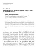
6. SCENARIO SIMULATION
To illustrate the principles shown in the previous sections, an
example has been selected as shown in Figure 14. The sce-
nario corresponds to a small office environment of 103
×
28 meters covered by three access points represented with
the lighter and darker shapes within the layout. The access
points are supposed to operate in IEEE802.11b + g, that is,
in g mode with backward compatibility to b.Tosimulate

the conditions as realistically as possible, the walls have been
modeled to introduce attenuation in the signal propagation
and edge diffraction.
The power levels that result in the scenario are also shown
as isolines in Figure 15 where darker shading corresponds to
higher signal strength. As can be seen, most of the interest
area in the scenario is within the
−80 dBm line, which is suf-
ficient to obtain maximum capacity with IEEEE802.11b + g.
To highlight the critical areas in the scenario, the peak
capacity has been estimated and shown in Figure 16.The
lighter areas represent the weaker signal conditions, that in
turn result in lower peak capacity in the scenario.
For the conversational video service, the approach fol-
lowed in previous sections could be compared with simu-
lation results of video capacity. The simulation consists of
running iterations that place a number of users in random
positions, ranging from a minimum number of users, to a
maximum one, and evaluating the number of call attempts
rejected by the call admission control for each value, because
of the congestion conditions and the field strength. The ra-
tio between the call attempts and the rejections is the outage
probability.
The overall process followed in the simulations is repre-
sented in Figure 17.
For each of the video configurations, the process starts
with a minimum number of simultaneous users. Uniform
random coordinates of users are generated to meet the num-
ber of users within the perimeter of the layout in Figure 14.
The next step in the process is to associate the clients to the

15 m
Figure 16: Simulation scenario peak available capacity.
Set number of
users
Random clients
generation
Client association
to AP
Client radio signal
quality estimation
Client assignment
to AP resources
Number of clients
in outage
Number
of iterations
reached
Average estimation
for the current
conditions
Maximum
number of users
reached
End
No
Ye s
No
Ye s
Figure 17: Simulations flow diagram.
access points. The association is based on signal strength; that

is, each of the clients will be linked to the AP with the better
radio link. Since the scenario is indoor, the association is not
necessarily correlated with the distance to the AP. For each
of the user’s coordinates p
i
, it is possible to find the power
received from the access points using
μ

j

x
i
, y
i

=

k
λ
k
+20log

max

1, d
j
(x, y)

, (36)

where μ

j

x
i
, y
i

represents the propagation losses at the user’s
coordinates p
i
to the j access points, λ
k
the attenuation of the
k crossed walls in the path from the user’s coordinates to the
base station, and d
j
the distances from the user’s coordinates
p
i
to the j access points. The average signal strength will then
be expressed as
S
j
= P
TX
+ G
TA
−l

T
−μ

j
+ G
RA
−l
R
, (37)
where P
TX
is the transmission power in dBm, G
TA
is the
gain of the transmission antenna in dBi, l
T
are the additional
losses in the transmission path before the antenna, G
RA
is the
gain of the receiving antenna, and l
R
are the additional losses
between the receiving antenna and the receiver.
The association of a user located at point p
i
will be to
the access point from which it receives the higher power level
Alfonso Fernandez-Duran et al. 13
Table 8: Simulation results for several outage probabilities.

Outage probability H.264 @ 64 Kbps H.264 @ 128 Kbps H.264 @ 384 Kbps 128 Kbps quality 384 Kbps quality
1% 94 48 12 29 6
5% 102 51 13 32 7
10% 105 54 15 34 8
Average simultaneous users per access point
Reference 36 19 6 13 3
1% 31 16 4 10 2
5% 34 17 4 11 2
10% 35 18 5 11 3
140120100806040200
Simultaneous users
0
10
20
30
40
50
60
70
80
90
100
Outage probability (%)
H.264@64 Kbps
H.264@128 Kbps
H.264@384 Kbps
128 Kbps quality
384 Kbps quality
Figure 18: Scenario simulation results.
between the j access points. This simple process can be mod-

eled as the j value for which power is
S
= max

S
j

. (38)
The association process in a multicell environment will also
fix the frequency channel used by the user client, and there-
fore it will condition the interaction with the rest of the cells.
The signal quality at each of the user positions is esti-
mated by using the resulting signal strength from (37)and
(38) with respect to the associated access point. The signal
quality in turn provides the working point for the particu-
lar client and then the resources needed for the video trans-
mission. In the case where the radio quality does not reach a
minimum threshold, the client is considered to be in an out-
age. The remaining clients are considered at their respective
working conditions to evaluate whether the total available re-
sources are enough to allocate all the video conversations. If
the resources are not enough, the number of clients is re-
duced till the video conversations fit in the system. The dif-
ference from the initial number of clients and the allocated
video conversations is the outage fraction of users. This pro-
cess is repeated several times for each number of clients rang-
ing in an interval that depends on the video mode used.
Following this approach, the results obtained are shown
in Figure 18, for the different types of video codecs.
Every point in Figure 18 is the average result of run-

ning similar condition over a large number of realizations,
and therefore the distributions of points follow exponential
trends as could be expected. The solid lines represent the
best-fit exponential trend for the sets of points.
From the outage probability curves, the maximum num-
ber of simultaneous video conversations could be obtained
for a given value of outage probability (typically between
1% and 10%). Figure 18 shows the network behavior for the
main video codecs, with the use of quality-related metrics in
the admission control (reduction of video frame rate).
Ta bl e 8 shows a summary of results from the scenario
simulation, where it can be seen that the total number of
simultaneous video calls estimated using the capacity ap-
proach (marked as reference) a bit higher than the one is ob-
tained in the simulation results. This is caused by the random
placement of video users in weaker propagation areas of the
scenario. It has to be noted that these results could be very
dependent on the particular scenario, and this is only taken
as an example.
7. CONCLUSIONS AND FUTURE WORK
Conversational video over wireless LAN dimensioning has
been addressed under the optimal network throughput and
the perspective of video quality. The paper proposes a sim-
ple and new dimensioning model that incorporates both key
aspects of throughput and quality.
The maximum number of simultaneous users due to
throughput is limited by the collisions taking place in the
shared medium with a statistical contention protocol. The
video quality is conditioned by the packet loss in the con-
tention protocol. Both approaches have been analyzed un-

der the scope of common conversational video profiles used
in conversational video applications over wireless LANs. The
approach presented is compatible and could be comple-
mented with radio propagation effects.
To illustrate the applicability of the dimensioning model
proposed, an office scenario has been simulated.
Subsequent research steps will be taken, to incorporate
the effects of handover in the conversational video perfor-
mance, as well as video quality indicators applicable to video
streaming and IPTV over WLAN.
14 EURASIP Journal on Wireless Communications and Networking
ACKNOWLEDGMENT
The authors are thankful to the support of the Spanish Min-
istry of Education and Science within the framework of
Project no. TEC2005-07010-C02-01/TCM.
REFERENCES
[1] Y. Koucheryavy, D. Moltchanov, and J. Harju, “Performance
evaluation of live video streaming service in 802.11b WLAN
environment under different load conditions,” in Proceedings
of the 1st International Workshop on Multimedia Interactive
Protocols and Systems (MIPS ’03), vol. 2899 of Lecture Notes
in Computer Science, pp. 30–41, Napoli, Italy, November 2003.
[2] T. Stockhammer, M. M. Hannuksela, and T. Wiegand,
“H.264/AVC in wireless environments,” IEEE Transactions on
Circuits and Systems for Video Technology,vol.13,no.7,pp.
657–673, 2003.
[3] A. Miu, J. G. Apostolopoulos, W. Tan, and M. Trott, “Low-
latency wireless video over 802.11 networks using path diver-
sity,” in Proceedings of the International Conference on Multi-
media and Expo (ICME ’03), vol. 2, pp. 441–444, Baltimore,

Md, USA, July 2003.
[4] E. Masala, C. F. Chiasserini, M. Meo, and J. C. De Martin,
“Real-time transmission of H.264 video over 802.11-based
wireless ad hoc networks,” in Proceedings of Workshop on DSP
in-Vehicular and Mobile Systems, pp. 193–207, Nagoya, Japan,
April 2003.
[5] ITU-T Recommendation G.1050, “Quality of service and
performance-generic and user related aspects network model
for evaluating multimedia transmission performance over In-
ternet Protocol,” November 2005.
[6] ITU-T Recommendation H.264, “Infrastructure of audiovi-
sual services-coding of moving video. Advanced video coding
for generic audiovisual services,” March 2005.
[7] Alcatel, “Open IMS solutions for innovative applications,”
White Paper, Ed. 7, November 2005.
[8] R. P
´
erez Leal and P. Cid Fern
´
andez, “Aplicaciones innovadoras
en el entorno IMS/TISPAN,” in Proceedings of Telecom I+D,p.
9, Madrid, Spain, November-December 2006.
[9] T. Wiegand, G. J. Sullivan, G. Bjøntegaard, and A. Luthra,
“Overview of the H.264/AVC video coding standard,” IEEE
Transactions on Circuits and Systems for Video Technology,
vol. 13, no. 7, pp. 560–576, 2003.
[10] ITU-T Recommendation H.241, “Infrastructure of audiovi-
sual services-communication procedures extended video pro-
cedures and control signals for H.300-series terminals,” May
2006.

[11] F. A. Tobagi, “Multiaccess protocols in packet communica-
tion systems,” IEEE Transactions on Communications Systems,
vol. 28, no. 4, pp. 468–488, 1980.
[12] R. Rom and M. Sidi, Multiple Access Protocols: Performance and
Analysis, Springer, New York, NY, USA, 1990.
[13] A. F. Fernandez and J. I. Alonso, “Method to estimate voice
over IP and data trafficcapacityinIEEEWLANs,”inInterna-
tional Workshop on Networks and Applications Towards a Ubiq-
uitously Connected World (EUNICE ’05), pp. 204–208, Madrid,
Spain, July 2005.
[14] S. W. Kim, B S. Kim, and Y. Fang, “Downlink and uplink re-
source allocation in IEEE 802.11 wireless LANs,” IEEE Trans-
actions on Vehicular Technolog y , vol. 54, no. 1, pp. 320–327,
2005.
[15] M. S. Gast, 802.11 Wireless Networks: The Definitive Guide,
O’Reilly Media, Sebastopol, Calif, USA, 2002.
[16] ISO/IEC 8802-11ANSI/IEEE Std 802.11 First Edition 1999-
00-00, “Information technology–telecommunications and in-
formation exchange between systems–local and metropolitan
area networks–specific requirements–part 11: wireless LAN
medium access control (MAC) and physical Layer (PHY) spec-
ifications,” 1999.
[17] K. Medepalli, P. Gopalakrishnan, D. Famolari, and T. Kodama,
“Voice capacity of IEEE 802.11b, 802.11a and 802.11g wireless
LANs,” in Proceedings of IEEE Global Telecommunications Con-
ference (GLOBECOM ’04), vol. 3, pp. 1549–1553, 2004.
[18] O. Awoniyi and F. A. Tobagi, “Effect of fading on the perfor-
mance of VOIP in IEEE 802.11 a WLANs,” in Proceedings of
IEEE International Conference on Communications, vol. 6, pp.
3712–3717, Paris, France, June 2004.

[19] D. P. Hole and F. A. Tobagi, “Capacity of an IEEE 802.11b
wireless LAN supporting VoIP,” in Proceedings of IEEE Inter-
national Conference on Communications, vol. 1, pp. 196–201,
Paris, France, June 2004.
[20] K. Medepalli, P. Gopalakrishnan, D. Famolari, and T. Kodama,
“Voice capacity of IEEE 802.11b and 802.11a wireless LANs in
the presence of channel errors and different user data rates,” in
Proceedings of the 60th IEEE Vehicular Technology Conference
(VTC ’04), vol. 60, pp. 4543–4547, Los Angeles, Calif, USA,
September 2004.
[21] N. Hegde, A. Prouti
`
ere, and J. Roberts, “Evaluating the voice
capacity of 802.11 WLAN under distributed control,” in Pro-
ceedings of the 14th IEEE Workshop on Local and Metropolitan
Area Networks (LANMAN ’05), pp. 6, September 2005.
[22] J. Hu, S. Choudhury, and J. D. Gibson, “PSNRr,f: assessment of
delivered AVC/H.264 video quality over 802.11a WLANs with
multipath fading,” in Proceedings of the 1st Multimedia Com-
munications Workshop (MULTICOMM ’06), pp. 1–6, Istam-
bul, Turkey, June 2006.
[23] S. Winkler, Digital Video Quality: Vision Models and Metrics,
John Wiley & Sons, New York, NY, USA, 2005, Genista Cor-
poration, Montreux (Switzerland).
[24] N. Feamster and H. Balakrishnan, “Packet loss recovery for
streaming video,” in Proceedings of the 12th International
Packet Video Workshop,pp.11,Pittsburgh,Pa,USA,April
2002.
[25] M. Horowitz, A. Joch, F. Kossentini, and A. Hallapuro,
“H.264/AVC baseline profile decoder complexity analysis,”

IEEE Transactions on Circuits and Systems for Video Technol-
ogy, vol. 13, no. 7, pp. 704–716, 2003.
[26] T. K. Sarkar, Z. Ji, K. Kim, A. Medouri, and M. Salazar-Palma,
“A survey of various propagation models for mobile commu-
nication,” IEEE Antennas and Propagation Magazine, vol. 45,
no. 3, pp. 51–82, 2003.
[27] H. Hashemi, M. McGuire, T. Vlasschaert, and D. Tholl, “Mea-
surements and modeling of temporal variations of the indoor
radio propagation channel,” IEEE Transactions on Vehicular
Technology, vol. 43, no. 3, pt. 1-2, pp. 733–737, 1994.
[28] F. Babich and G. Lombardi, “Statistical analysis and character-
ization of the indoor propagation channel,” IEEE Transactions
on Communications, vol. 48, no. 3, pp. 455–464, 2000.
[29] O. A. Lotfallah, M. Reisslein, and S. Panchanathan, “A frame-
work for advanced video traces: evaluating visual quality for
video transmission over lossy networks,” EURASIP Journal on
Applied Signal Processing, vol. 2006, Article ID 42083, 21 pages,
2006.