Báo cáo hóa học: " Research Article An Ultradiscrete Matrix Version of the Fourth Painlevé Equation" pptx

Hindawi Publishing Corporation
Advances in Difference Equations
Volume 2007, Article ID 96752, 14 pages
doi:10.1155/2007/96752
Research Article
An Ultradiscrete Matrix Version of the Fourth Painlevé Equation
Chris M. Field and Chris M. Ormerod
Received 27 February 2007; Accepted 1 May 2007
Recommended by Kilkothur Munirathinam Tamizhmani
This paper is concerned with the matrix gener alization of ultradiscrete systems. Specif-
ically, we establish a matrix generalization of the ultradiscrete fourth Painlev
´
e equation
(ud-P
IV
). Well-defined multicomponent systems that permit ultradiscretization are ob-
tained using an approach that relies on a group defined by constraints imposed by the
requirement of a consistent evolution of the systems. The ultradiscrete limit of these sys-
tems yields coupled multicomponent ultradiscrete systems that generalize ud-P
IV
.The
dynamics, irreducibility, and integrability of the matrix-valued ultradiscrete systems are
studied.
Copyright © 2007 C. M. Field and C. M. Ormerod. This is an open access ar ticle distrib-
uted under the Creative Commons Attribution License, which permits unrestricted use,
distribution, and reproduction in any medium, provided the original work is properly
cited.
1. Introduction
Discrete Painlev
´
e equations are difference equation analogs of classical Painlev

´
e equa-
tions [1] and have been extensively studied recently (see the rev iew article [2]). The ul-
tradiscrete Painlev
´
e equations are discrete equations considered to be extended cellular
automata (they may also be considered as piecewise linear systems) that are derived by
applying the ultradiscretization process [3] to discrete Painlev
´
e equations. This process
has been accepted as one that preserves integrability [4]. Particular indicators of inte-
grability in the ultradiscrete setting include the existence of a Lax pair [5], an analog of
singularity confinement [6], and special solutions [7].
All of the preceding examples arising from ultradiscretization are one-component (i.e.,
scalar) systems. Generalizations of integrable systems to associative a lgebras have been
considered for many years (see [8] and referencestherein). However, the general methods
2AdvancesinDifference Equations
and results prev iously obtained are inapplicable in the ultradiscrete setting, due to the
requirement of a subtraction free setting. We present for the first time a matrix general-
ization of an ultr adiscrete system. Without wishing to labour the point, let us st ress again
that, the issue of mat rix generalizations of ultradiscrete systems is a separate, more technical
issue, than that of the matrix generalization of the original discrete systems. T his is the issue
which we are concerned with here.
The constraints related to the subtraction free setting and consistent evolution are
studied in a group theoretic approach, in which one may also describe the nature of the
irreducible subsystems. As an application of this method, we introduce a matrix version
of the ud-P
IV
of [9] which is derived by applying the ultradiscretization procedure to
q-P

IV
:
f
0
(qt) = a
0
a
1
f
1
(t)
1+a
2
f
2
(t)+a
2
a
0
f
2
(t) f
0
(t)
1+a
0
f
0
(t)+a
0

a
1
f
0
(t) f
1
(t)
,
f
1
(qt) = a
1
a
2
f
2
(t)
1+a
0
f
0
(t)+a
0
a
1
f
0
(t) f
1
(t)

1+a
1
f
1
(t)+a
1
a
2
f
1
(t) f
2
(t)
,
f
2
(qt) = a
1
a
2
f
0
(t)
1+a
1
f
1
(t)+a
1
a

2
f
1
(t) f
2
(t)
1+a
2
f
2
(t)+a
0
a
2
f
0
(t) f
2
(t)
.
(1.1)
With the explicit form of the matrices derived, the new systems can be considered as
coupled multicomponent generalizations. It should be stressed that the approach of this
paper gives all possible ultradiscretizable matrix-valued versions of (1.1).
The reason for choosing q-P
IV
is that it has already been thoroughly and expertly in-
vestigated in the scalar case (i.e., when f
i
and a

i
are scalar) [9]. In [9], q-P
IV
was shown
to admit the action of the affine Weyl group of type A
(1)
2
as a group of B
¨
acklund t ransfor-
mations, to have classical solutions expressible in terms of q-Hermite-Weber functions,
to have rational solutions, and its connection with the classification of Sakai [10] was also
investigated. Furthermore, the ultradiscrete limit was taken in [9 ], and was shown to also
admit affine Weyl group representations. As q-P
IV
is such a rich system, and has already
been well studied, this makes it a perfect system for the application of our approach of
ultradiscrete matr ix generalization.
Before turning to the derivation of matrix ud-P
IV
, ultradiscretization should be int ro-
duced in more detail, so that the reason for certain constraints given later will be clear.
The process is a way of bringing a rational expression, f , in variables (or parameters)
a
1
, ,a
n
to a new expression, F, in new ultradiscrete variables A
1
, ,A

n
, that are related
to the old variables via the relation a
i
= e
A
i
/
and limiting process
F

A
1
, ,A
n

=
lim
→0
 log f

a
1
, ,a
n

. (1.2)
In general it is sufficient to make the following correspondences between binary opera-
tions
a +b

−→ max (A,B),
ab
−→ A + B,
a/b
−→ A − B.
(1.3)
C. M. Field and C. M. Ormerod 3
This process is a way in which we may take an integrable mapping over the positive real
numbers
R
+
to an integrable mapping over the max-plus semiring [11]. The requirement
that the pre-ultradiscrete equations are subtraction free expressions of a definite sign is a
more stringent restraint in the matrix setting than the one-component setting, and it is
this requirement which motivates the particular form of our matrix system.
The outline of this paper is as follows. In Section 2,aq-P
IV
is derived in the noncom-
mutative setting, where the dependent variables take their values in an associative algebra.
In Section 3 conditions on the matrix forms of the dependent variables and parameters
of q-P
IV
are derived such that it has a well-defined evolution and is ultradiscretizable.
The group theoretic approach is adopted to describe the constraints on the system. In
Section 4 the ultradiscrete version of this system is derived, and some of the rich phe-
nomenology of the der ived matrix-valued ultradiscrete P
IV
is displayed and analyzed in
Section 5.
2. Symmetric q-P

IV
on an associative algebra
In this section it is shown that the symmetric q-P
IV
of [9]canbederivedfromaLax
formalism in the noncommutative setting, where the dependent variables
{ f
i
} take values
in an a priori arbitrary associative algebra, Ꮽ,withunitI over a field
K (when we turn
to ultradiscretization, the requirement of a field will be modified, but not in such a way
as to affect the derivation from a Lax pair). This puts the present work in the context
of other recent works on integrable systems such as [8, 12] where the structure of inte-
grable ODEs and PDEs (resp.) was extended to the domain of associative algebras, and
[13] where Painlev
´
e equations were defined on an associative algebra (see also [8]). This
trend has also been present in works on discrete integrable systems such as [14]where
the higher dimensional consistency (consistency around a cube) property was investi-
gated for integrable partial difference equations defined on an associative algebra, and
[15] where an initial value problem on the lattice KdV with dependent variables taking
values in an associative algebra was studied, leading to exact solutions.
The auxiliary (spectral) parameter x, time variable t, and constant q belong to the field
K. The dependent variables { f
i
}∈Ꮽ, system parameters {b
i
}∈Ꮽ (i ∈{0,1,2}), and we
define

Γ
i
:= I + b
3
i
f
i
+ b
3
i
b
3
i+1
f
i
f
i+1
(2.1)
up to an arbitrary ordering of the b
3
j
and f
j
factors. (It will be shown that the ordering
of these factors within Γ
i
is of no consequence for either the integrability of the system
or the existence of a well-defined evolution in the ultradiscrete limit.) The invertibility of
these expressions is assumed, that is Γ
−1

i
∈ Ꮽ.
We derive the system from a linear problem to settle other ordering issues in the non-
commutative setting. The q-type Lax formalism is given by
φ(qx, t)
= L(x,t)φ(x,t), φ(x,qt) = M(x,t)φ(x,t), (2.2)
4AdvancesinDifference Equations
where
L(x,t)
=
⎛
⎜
⎜
⎝

1+x
2

Ib
0
f
0
t
−2/3
0
0

1+x
2


Ib
1
f
1
t
−2/3
b
2
f
2
t
−2/3
0

1+x
2

I
⎞
⎟
⎟
⎠
,
M(x,t)
=
⎛
⎜
⎜
⎝
0 b

−2
2
Γ
2
0
00b
−2
0
Γ
0
b
−2
1
Γ
1
00
⎞
⎟
⎟
⎠
.
(2.3)
The ultradiscrete version of this linear problem (for the usual commutative case) origi-
nally appeared in [16].
The compatibility condition for this linear problem reads
M(qx,t)L(x,t)
= L(x,qt)M(x,t), (2.4)
and leads to
b
0

f
0
= q
2/3
b
−2
2
Γ
2
b
1
f
1
Γ
−1
0
b
2
0
,
b
1
f
1
= q
2/3
b
−2
0
Γ

0
b
2
f
2
Γ
−1
1
b
2
1
,
b
2
f
2
= q
2/3
b
−2
1
Γ
1
b
0
f
0
Γ
−1
2

b
2
2
,
(2.5)
where t he overline denotes a time update and
b
i
= b
i
.
Following [9], we show that a product of the dependent variables can be regarded as
the independent variable. With
{ f
−1
i
}∈Ꮽ, {b
−1
i
}∈Ꮽ (i.e., we are working with a skew
field) and specifying that the product b
0
f
0
b
1
f
1
b
2

f
2
is proportional to I,itisseenthat
b
0
f
0
b
1
f
1
b
2
f
2
= qc
2
I where c ∈ K and c = qc. Without loss of generality we set c = t.From
now on
b
0
f
0
b
1
f
1
b
2
f

2
= qt
2
I (2.6)
will be imposed (so the algebra generated by all three
{ f
i
} and I is not free). The in-
vertibility of the algebra elements
{ f
i
} and {b
i
} is a consequence of the explicit matrix
representation of these objects for the well-defined matrix systems studied in the next
sections.
With the restriction
b
3
0
b
3
1
b
3
2
= qI (2.7)
imposed, the map (2.5) is a noncommuting generalization of q-P
IV
. If we specify that b

i
and f
i
be matrix valued, the only requirement for a consistent evolution is that the Γ
i
are
invertible. This system however is too general to be ultradiscretized, since in gener al we
require the inverse to b e subtraction free.
If all variables commute, then after the change of variables a
i
:= b
3
i
the map reduces to
q-P
IV
,(1.1), as presented in [9].
C. M. Field and C. M. Ormerod 5
3. Ultradiscret izable matrix str ucture
The conditions (2.6)and(2.7) can be used in conjunction with (2.5) to define constraints
that lead to a consistent evolution on Ꮽ as a free algebra with two-constant (say b
1
and
b
2
) and two-variable (say f
1
and f
2
) generators. Regarding these as n × n (or even infinite

dimensional) matrices leads to multicomponent systems. However, the aim of the present
work is to derive matrix (or multicomponent) ultradiscrete systems, and hence, as we
require the expressions to be subtraction free, we have considerably less freedom than
this general setting.
Due to this restriction, we restrict Ꮽ to be the group of invertible nonnegative matri-
ces, that is, we set
Ꮽ
= S
n
 K
n
, (3.1)
where S
n
is the symmetric group and K will further be restricted to be R
+
in models where
we wish to perform ultradiscretization. For our purposes S
n
is realized as n × n matrices
of the form δ
iσ(j)
for σ ∈ S
n
. (This group decomposition result can been seen in [17].) We
define the homomorphism π : Ꮽ
→ Ꮽ/K
n
= S
n

to be the homomorphism obtained as a
result of the above semidirect product. This allows us to more easily deduce the form of
the matrices
{ f
i
}, {b
i
},thatgiveawell-definedevolution.
Since Ꮽ is a semidirect product, the elements b
i
and f
i
can be uniquely written in the
form
b
i
= β
i
s
i
,
f
i
(t) = 
i
(t)z
i
,
(3.2)
where π(b

i
) = s
i
∈ S
n
, π( f
i
(t)) = z
i
∈ S
n
,andβ
i
and 
i
(t) are diagonal matr ices contain-
ing the n components of b
i
and f
i
(t), respectively (we leave the matrix representation
implicit).
We now derive further restrictions on
{s
i
} and {z
i
} such that the evolution is consis-
tent, and all terms in the map (such as the Γ
i

)remaininᏭ,(3.1).
Consider the following form of Γ
i
Γ
i
:= I + b
3
i
f
i
+ b
3
i
b
3
i+1
f
i+1
f
i
. (3.3)
As π(I)
= I, π(Γ
i
) = I and this implies
s
3
i
z
i

= Ii∈{0,1,2}. (3.4)
This is the only condition that arises f rom the requirement that Γ
i
∈ Ꮽ,whereᏭ is given
by (3.1). It is immediately seen that condition (3.4) is independent of the ordering of
the b
3
i
f
i
term in Γ
i
. There are 24 possible orderings of b
3
i
b
3
i+1
f
i+1
f
i
(we do not consider
the possibility of splitting up the b
i
factors, as b
3
i
=: a
i

is the parameter in the commu-
tative case [9]). Of these 24 possibilities, 8 also require the commutativity of s
3
i
and s
3
j
(equivalently z
i
and z
i+1
). It is shown in the appendix that these additional commutativ-
ity relations do not change the restrictions on
{s
i
} and {z
i
}. (That is, commutativit y of s
3
i
and s
3
j
is a consequence of the full set of relations.)
6AdvancesinDifference Equations
Requiring the preservation of (3.2)asthevariablesevolve,theprojectionof(2.5)onto
S
n
,with(3.4), gives
s

4
i
= s
2
i+1
s
2
i
−1
i ∈{0,1,2}. (3.5)
The projection of the constraints (2.6)and(2.7)ontoS
n
,with(3.4), gives
s
2
2
s
2
1
s
2
0
= I, (3.6)
s
3
0
s
3
1
s

3
2
= I, (3.7)
respectively.
Therefore, to give a consistent evolution that permits ultradiscretization, {s
i
} are ho-
momorphic images of the group generators of
G
=

g
0
,g
1
,g
2
| g
4
0
= g
2
1
g
2
2
, g
4
1
= g

2
2
g
2
0
, g
4
2
= g
2
0
g
2
1
, g
2
2
g
2
1
g
2
0
= 1, g
3
0
g
3
1
g

3
2
= 1

(3.8)
in S
n
; {z
i
} are given by (3.4). The group G has order 108. The order of the generators of
G is shown to be 18 in the appendix.
4. Ultradiscret ization
We now consider the ultradiscretization of the matrix-valued systems derived in the pre-
vious section. The components of the ultradiscretized systems belong to the max-plus
semiring, S, which is the set
R ∪ {−∞} adjoined with the binary operations of max and +
(often called tropical addition and tropical multiplication). To map the pre-ultradiscrete
expression to the max-plus semiring, we may simply make the correspondences (1.3)on
the level of the components. (So
−∞ becomes the additive identity and 0 becomes the
multiplicative identity.) By ultradiscretizing matrix oper ations, we arrive at the following
definitions of matrix operations over S.IfA
= (a
ij
)andB = (b
ij
), then following [5], we
define tropical matrix addition and multiplication,
⊕ and ⊗, by the equations
(A

⊕ B)
ij
:= max

a
ij
,b
ij

,
(A
⊗ B)
ij
:= max
k

a
ik
+ b
kj

,
(4.1)
along with a scalar operation given by
(λ
⊗ A)
ij
:=

λ + a

ij

(4.2)
for all λ
∈ S. In the ultradiscrete limit 0 is mapped to −∞,and1ismappedto0;hence
the identity matrix, I, is the matrix with zeros along the diagonal and
−∞ in every other
entry. In the same way it is clear what happens to matrix realizations of members of S
n
in
the ultradiscrete limit.
An ultradiscretized member of the group Ꮽ,(3.1), has a decomposition of the form
D
= Δ ⊗ T (4.3)
C. M. Field and C. M. Ormerod 7
(cf. (3.1)) where Δ has
−∞ for all off-diagonal entries and T is an ultradiscretization of
an element of S
n
.Itsinverseisgivenby
D
−1
= T
−1
⊗ Δ
−1
, (4.4)
where (Δ
−1
)

ii
≡−(Δ)
ii
and all off-diagonal entries are −∞.
As well as the matr ix map, the correspondence also allows us to easily write the Lax
pair over the semialgebra
ᏸ(X,T)
=
⎛
⎜
⎜
⎜
⎜
⎜
⎝
max(0,2X) ⊗ IB
0
⊗ F
0
⊗−
2T
3
−∞
−∞
max(0,2X) ⊗ IB
1
⊗ F
1
⊗−
2T

3
B
2
⊗ F
2
⊗−
2T
3
−∞ max(0,2X) ⊗ I
⎞
⎟
⎟
⎟
⎟
⎟
⎠
,
ᏹ(X,T)
=
⎛
⎜
⎝
−∞
B
−2
2
⊗ Γ
2
−∞
−∞ −∞

B
−2
0
⊗ Γ
0
B
−2
1
⊗ Γ
1
−∞ −∞
⎞
⎟
⎠
,
(4.5)
where t he ultradiscretization of Γ
i
,asgivenin(2.1), is the matrix
Γ
i
= I ⊕

B
3
i
⊗ F
3
i


⊕

B
3
i
⊗ B
3
i+1
⊗ F
i
⊗ F
i+1

. (4.6)
The compatibility condition reads
ᏹ(X + Q,T)
⊗ ᏸ(X,T) = ᏸ(X,T + Q) ⊗ ᏹ(X,T) (4.7)
and gives the ult radiscrete equation over an associative S-algebra
B
0
⊗ F
0
=
2
3
Q
⊗ B
−2
2
⊗ Γ

2
⊗ B
1
⊗ F
1
⊗ Γ
−1
0
⊗ B
2
0
,
B
1
⊗ F
1
=
2
3
Q
⊗ B
−2
0
⊗ Γ
0
⊗ B
2
⊗ F
2
⊗ Γ

−1
1
⊗ B
2
1
,
B
2
⊗ F
2
=
2
3
Q
⊗ B
−2
1
⊗ Γ
1
⊗ B
0
⊗ F
0
⊗ Γ
−1
2
⊗ B
2
2
.

(4.8)
The ultradiscrete versions of the restrictions (2.6)and(2.7)are
B
0
⊗ F
0
⊗ B
1
⊗ F
1
⊗ B
2
⊗ F
2
= (Q +2T) ⊗ I,
B
3
0
⊗ B
3
1
⊗ B
3
2
= Q ⊗ I.
(4.9)
(Of course, it would have been equally legitimate to apply the correspondence on the level
of the map (2.5) without starting from a derivation from the ultradiscretized Lax pair.)
It is easily seen t hat if 2Q/3, the parameter T, and all components of the map belong
to

Z then at all time steps all components (not formally equal to −∞)belongtoZ.Itis
this property which motivates the term “extended cellular automata.”
8AdvancesinDifference Equations
5. Phenomenology
As mentioned in the above discussion, we are required to find homomorphic images of
the group G in S
n
. To do this, we use the computer algebra package Magma. The homo-
morphic images of G in S
n
give rise to reducible and irreducible subgroups, which in turn
translate to reducible and irreducible matrix-valued systems. By definition, the reducible
systems are decomposable into irreducible systems, and hence we restrict our attention
to the ir reducible cases.
We may use any homomorphism to induce a group action of G onto a set of n objects.
In this manner, we may state by the orbit stabilizer theorem that the size of any orbit
of G must divide the order of the group. Since the group has order 108, this implies the
irreducible images of G to be of sizes that divide 108. In terms of matrix-valued systems,
the implication is that any irreducible matrix-valued systems are of sizes that divide 108.
The lowest-rank cases of the homomorphic images of the generators of G in S
n
are
given in Ta b le 5.1 using the standard cycle notation for the symmetric group. The rank 1
case is well understood [9]; hence we turn to the rank 2 case. For the examples presented
here, we restrict our attention to the ordering within the
{Γ
i
},(4.6).
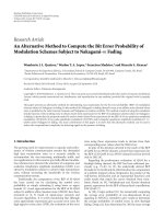
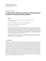
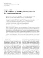
Typical behavior of t he rank 2 map is shown in Figure 5.1. The initial conditions and
parameter values in this case are

B
0
=

−∞
0
0
−∞

, B
1
=
⎛
⎝
−∞
0
4
5
−∞
⎞
⎠
,
F
0
=

−∞
0
0
−∞


, F
1
=

−∞
0
0
−∞

,
(5.1)
where B
2
and F
2
are determined by the constraints, and Q = 1. For most initial conditions
and parameter values, the behavior has a similar level of visual complexity.
It is a hallmark of the integrability of Painlev
´
e systems that they possess special solu-
tions such as rational and hypergeometric functions [18]. A remarkable discovery of our
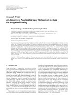
numerical investigations is that (4.8) displays special solution type behavior. These solu-
tions only occur for specific parameter values and initial conditions. One example of this
comes at a surprisingly close set of parameters and initial conditions to those displayed
in Figure 5.1. By setting the parameters to be
B
0
=


−∞
0
0
−∞

, B
1
=
⎛
⎝
−∞
0
3
5
−∞
⎞
⎠
, (5.2)
with the same set of initial conditions, the behavior coalesces down to the much simpler
form shown in Figure 5.2.
The graphs of the single components in Figure 5.2 strongly resemble the recently dis-
covered ultradiscrete hypergeometric functions of [7]. This implies that the special solu-
tion behavior shown here may be parameterized by a higher-dimensional generalization
of the ultradiscrete hypergeomet ric functions of [7]. We discuss this possibility further in
Section 6. Behavior resembling rational solutions has also been observed in our compu-
tational investigations.
C. M. Field and C. M. Ormerod 9
Table 5.1. Lowest-rank cases of homomorphic images of the generators of G in S
n
written in cycle

notation.
Rank g
0
g
1
g
2
1 111
2
(1,2) (1, 2) 1
3
(1,2,3) (1,2,3) (1,2,3)
(1,2,3) (1,3,2) 1
4
(1,2)(3,4) (1,3)(2,4) (1,4)(2,3)
6
(1,2,3,4,5,6) (1,6,5,4,3, 2) 1
(1,2)(3,4)(5,6) (1,3,6)(2,4,5) (1,5,3,2, 6,4)
(1,2,3)(4,5,6) (1,4,3,6,2,5) (1,4,3,6,2,5)
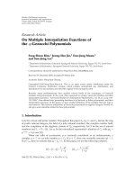
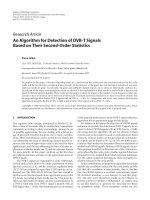
The typical behavior of the rank-3 map is shown in Figure 5.3. The initial conditions
and parameter values are
B
0
=
⎛
⎜
⎜
⎜
⎜
⎝

−∞
1
5
−∞
−∞ −∞
1
4
−3 −∞ −∞
⎞
⎟
⎟
⎟
⎟
⎠
, B
1
=
⎛
⎜
⎜
⎜
⎜
⎜
⎝
−∞ −∞
1
7
3
5
−∞ −∞

−∞ −
1
2
−∞
⎞
⎟
⎟
⎟
⎟
⎟
⎠
,
F
0
=
⎛
⎜
⎜
⎝
−
2 −∞ −∞
−∞
1 −∞
−∞ −∞
3
⎞
⎟
⎟
⎠
, F

1
=
⎛
⎜
⎜
⎜
⎝
−
1
4
−∞ −∞
−∞ −
5 −∞
−∞ −∞
1
⎞
⎟
⎟
⎟
⎠
,
(5.3)
where t he coupling comes from the forms of the parameters.
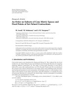
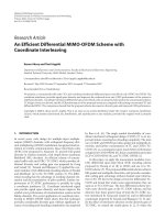
We also find behavior which we conjecture to be parameterized by higher-dimensional
ultradiscrete hypergeometric functions. For initial conditions and parameters
B
0
=
⎛
⎜

⎜
⎝
−∞
0 −∞
−∞ −∞
0
0
−∞ −∞
⎞
⎟
⎟
⎠
, B
1
=
⎛
⎜
⎜
⎜
⎝
−∞ −∞
0
3
5
−∞ −∞
−∞
0 −∞
⎞
⎟
⎟

⎟
⎠
,
F
0
=
⎛
⎜
⎜
⎝
0 −∞ −∞
−∞
0 −∞
−∞ −∞
0
⎞
⎟
⎟
⎠
, F
1
=
⎛
⎜
⎜
⎝
0 −∞ −∞
−∞
0 −∞
−∞ −∞

0
⎞
⎟
⎟
⎠
(5.4)
we obtain the behavior exhibited in Figure 5.4.
6. Conclusions and discussion
We have presented a noncommutative generalization of q-P
IV
. Conditions were derived
such that the matrix-valued systems could be ultradiscretized. In Section 4, the matrix
generalization of ultradiscrete P
IV
was presented. In Section 5, a small snapshot of the
10 Advances in Difference Equations
40
30
20
10
10
20
5
10 15 20
(a) F
0
: both components
40
30
20

10
10
20
5101520
(b) F
1
: both components
40
30
20
10
10
5101520
(c) F
2
: both components
Figure 5.1. Generic behavior of the rank-2 case. Component values are plotted against time step
values.
30
20
10
10
5101520
(a) F
0
: both components
30
25
20
15

10
5
5101520
(b) F
1
: both components
20
15
10
5
5
5
10 15 20
(c) F
2
: both components
Figure 5.2. Some special behavior of the rank-2 case.
C. M. Field and C. M. Ormerod 11
30
20
10
5101520
(a) F
0
: all 3 components
30
20
10
5101520
(b) F

1
: all 3 components
30
20
10
5101520
(c) F
2
: all 3 components
Figure 5.3. Generic behavior of the rank-3 case.
17.5
15
12.5
10
7.5
5
2.5
5101520
(a) F
0
: all 3 components
17.5
15
12.5
10
7.5
5
2.5
5101520
(b) F

1
: all 3 components
17.5
15
12.5
10
7.5
5
2.5
5101520
(c) F
2
: all 3 components
Figure 5.4. Some special behavior of the rank-3 case.
12 Advances in Difference Equations
rich phenomenology was presented. Due to space restr ictions, only certain aspects of this
phenomenology was presented, yet our preliminary findings suggest many avenues for
future research, including the generalization of the results in [7] to higher-dimensional
ultradiscrete hypergeometric functions.
In [19] Grammaticos et al. explicitly related two different forms of a q-discrete analog
of P
V
, and clarified the relationship from the point of view of affine Weyl group theory. It
would be illuminating to see how the construction of this paper is modified when applied
to different equations that are in fact the same system.
It is worth noting that a different generalization of q-P
IV
has been studied by Kajiwara
et al. [20, 21]. It would be interesting to know how both generalizations can be combined.
Appendix

Miscellaneous properties of the group G
By deducing properties of the group G presented in (3.8), we may deduce properties of
our elements
{s
i
} and {z
i
} since the {s
i
} must be homomorphic images of the generators
of G, while the
{z
i
} are determined by the {s
i
} via (3.4).
Proposition A.1.
g
6
0
= g
6
1
= g
6
2
. (A.1)
Proof. Constraint (3.5) implies
g
2

2
= g
−2
1
g
4
0
= g
4
1
g
−2
0
. (A.2)
Therefore g
6
0
= g
6
1
, and similarly we have the full proof. 
(Note that this implies [g
i
,g
6
j
] = 0.)
Proposition A.2. Group elements
{g
i

} have order 18.
Proof. As g
6
1
= g
6
0
it follows from constraints (3.5)and(3.6)that
g
8
0
= g
2
2
g
2
0
g
−2
2
. (A.3)
Hence
g
24
0
= g
2
2
g
6

0
g
−2
2
= g
6
0
,(A.4)
and therefore
g
18
0
= I. (A.5)
The proofs of
g
18
1
= I, g
18
2
= I (A.6)
proceed in the same manner.

C. M. Field and C. M. Ormerod 13
Proposition A.3.

g
3
i
,g

3
j

=
0. (A.7)
Proof. Using (A.1), (3.7) shows us that
g
6
0
= g
−3
1
g
−3
0
g
−3
1
g
−3
0
,(A.8)
further application of (A.1) reveals that
g
9
0
= g
−6
0
g

3
1
g
−3
0
g
−3
1
,(A.9)
hence, using (A.5),
g
−3
0
g
3
1
= g
3
1
g
−3
0
. (A.10)
Thereforewehavethecommutativityofg
3
0
and g
3
1
, and similarly we obtain (A.7). 

Acknowledgments
The authors wish to thank Nalini Joshi for discussions on discrete Painlev
´
e equations and
ultradiscretization, and Stewart Wilcox for useful correspondence. C. M. Field is sup-
ported by the Aust ralian Research Council Discovery Project Grant #DP0664624. The
research of C. M. Ormerod was supported in part by the Aust ralian Research Council
Grant #DP0559019.
References
[1] P. Painlev
´
e, “M
´
emoire sur les
´
equations diff
´
erentielles dont l’int
´
egrale g
´
en
´
erale est uniforme,”
Bulletin de la Soci
´
et
´
eMath
´

ematique de France, vol. 28, pp. 201–261, 1900.
[2] B. Grammaticos and A. Ramani, “Discrete Painlev
´
e equations: a review,” in Discrete Integrable
Systems, vol. 644 of Lecture Notes in Phys., pp. 245–321, Springer, Berlin, Germany, 2004.
[3] T. Tokihiro, D. Takahashi, J. Matsukidaira, and J. Satsuma, “From soliton equations to integrable
cellular automata through a limiting procedure,” Physical Review Letters, vol. 76, no. 18, pp.
3247–3250, 1996.
[4] S. Isojima, B. Grammaticos, A. Ramani, and J. Satsuma, “Ultradiscretization without positivity,”
Journal of Physics A, vol. 39, no. 14, pp. 3663–3672, 2006.
[5] G. R. W. Quispel, H. W. Capel, and J. Scully, “Piecewise-linear soliton equations and piecewise-
linear integrable maps,” Journal of Physics A, vol. 34, no. 11, pp. 2491–2503, 2001.
[6] N. Joshi and S. Lafortune, “How to detect integrability in cellular automata,” Journal of Physics
A, vol. 38, no. 28, pp. L499–L504, 2005.
[7] C. M. Ormerod, “Hypergeometric solutions to ultradiscrete Painlev
´
e equations,” preprint, 2006,
/>[8] P. J. Olver and V. V. Sokolov, “Integrable evolution equations on associative algebras,” Commu-
nications in Mathematical Physics, vol. 193, no. 2, pp. 245–268, 1998.
[9] K. Kajiwara, M. Noumi, and Y. Yamada, “A study on the fourth q-Painlev
´
e equation,” Journal of
Physics A, vol. 34, no. 41, pp. 8563–8581, 2001.
[10] H. Sakai, “Rational surfaces associated with affine root systems and geometry of the Painlev
´
e
equations,” Communications in Mathematical Physics, vol. 220, no. 1, pp. 165–229, 2001.
14 Advances in Difference Equations
[11] B. Grammaticos, Y. Ohta, A. Ramani, D. Takahashi, and K. M. Tamizhmani, “Cellular automata
and ultra-discrete Painlev

´
e equations,” Physics Letters A, vol. 226, no. 1-2, pp. 53–58, 1997.
[12] A. V. Mikhailov and V. V. Sokolov, “Integrable ODEs on associative algebras,” Communications
in Mathematical P hysics, vol. 211, no. 1, pp. 231–251, 2000.
[13] S. P. Balandin and V. V. Sokolov, “On the Painlev
´
e test for non-abelian equations,” Physics Letters
A, vol. 246, no. 3-4, pp. 267–272, 1998.
[14] A. I. Bobenko and Yu. B. Suris, “Integrable noncommutative equations on quad-graphs. The
consistency approach,” Letters in Mathematical Physics, vol. 61, no. 3, pp. 241–254, 2002.
[15] C. M. Field, F. W. Nijhoff, and H. W. Capel, “Exact solutions of quantum mappings from the
lattice KdV as multi-dimensional operator difference equations,” JournalofPhysicsA, vol. 38,
no. 43, pp. 9503–9527, 2005.
[16] N. Joshi and C. M. Ormerod, “The general theory of linear difference equations over the invert-
ible max-plus algebra,” Stud. Appl. Math. 118, no. 1, pp. 85–97, 2007.
[17] E. I. Bunina and A. V. Mikhal
¨
ev, “Automorphisms of the semigroup of invertible matrices with
nonnegative elements,” Fundamental’naya i Prikladnaya Matematika, vol. 11, no. 2, pp. 3–23,
2005.
[18] A. Ramani, B. Grammaticos, T. Tamizhmani, and K. M. Tamizhmani, “Special function solu-
tions of the discrete Painlev
´
e equations,” Computers & Mathematics with Applications, vol. 42,
no. 3–5, pp. 603–614, 2001.
[19] B. Grammaticos, A. Ramani, and T. Takenawa, “On the identity of two q-discrete Painlev
´
e
equations and their geometrical derivation,” Advances in Difference Equations, vol. 2006, Article
ID 36397, 11 pages, 2006.

[20] K. Kajiwara, M. Noumi, and Y. Yamada, “Discrete dynamical systems with W(A
(1)
m
−1
× A
(1)
n
−1
)
symmetry,” Letters in Mathematical Physics, vol. 60, no. 3, pp. 211–219, 2002.
[21] K.Kajiwara,M.Noumi,andY.Yamada,“q-Painlev
´
e systems arising from q-KP hierarchy,” Let-
ters in Mathematical Physics, vol. 62, no. 3, pp. 259–268, 2002.
Chris M. Field: School of Mathematics and Statistics F07, The University of Sydney,
Sydney NSW 2006, Australia
Email address: cmfi
Chris M. Ormerod: School of Mathematics and Statistics F07, The University of Sydney,
Sydney NSW 2006, Australia
Email address: