Báo cáo hóa học: " Research Article Mean-Square Performance Analysis of the Family of Selective Partial Update NLMS and Affine Projection Adaptive Filter Algorithms in Nonstationary Environment" doc

Hindawi Publishing Corporation
EURASIP Journal on Advances in Signal Pr ocessing
Volume 2011, Article ID 484383, 11 pages
doi:10.1155/2011/484383
Research Ar ticle
Mean-Square Performance Analysis of the Family of
Selective Partial Update NLMS and Affine Projection Adaptive
Filter Algorithms in Nonstationary Environment
Mohammad Shams Esfand Abadi and Fatemeh Moradiani
Faculty of Electrical and Computer Engineering, Shahid Rajaee Teacher Training University, P.O. Box 16785-163, Tehran, Ir an
Correspondence should be addressed to Mohammad Shams Esfand Abadi,
Received 30 June 2010; Revised 29 August 2010; Accepted 11 October 2010
Academic Editor: Antonio Napolitano
Copyright © 2011 M. Shams Esfand Abadi and F. Moradiani. This is an open a ccess article distributed under the Creative
Commons Attribution License, which permits unrestricted use, distribution, and reproduction in any medium, provided the
original work is properly cited.
We present the general framework for mean-square performance analysis of the selective partial update affine projection algorithm
(SPU-APA) and the family of SPU normalized least mean-squares (SPU-NLMS) adaptive filter algorithms in nonstationary
environment. Based on this the tracking performance of Max-NLMS, N-Max NLMS and the various types of SPU-NLMS and
SPU-APA can be analyzed in a unified way. The analysis is based on energy conservation arguments and does not need to assume
a Gaussian or white distribution for the regressors. We demonstrate through simulations that the derived expressions are useful in
predicting the performances of this family of adaptive filters in nonstationary environment.
1. Introduction
Mean-square performance analysis of adaptive filtering algo-
rithms in nonstationary environments has been, and still is,
an area of active research [1–3]. When the input signal
properties vary with time, the adaptive filters are able to track
these variations. The aim of tracking performance analysis
is to characterize this tracking ability in nonstationary
environments. In this area, many contributions focus on
a particular algorithm, making more or less restrictive

assumptions on t he input signal. For example, in [4, 5 ],
the transient performance of the LMS was presented in the
nonstationary en vironments. The former uses a random-
walk model for the variations in the optimal weight vector,
while the latter assumes deterministic variations in the
optimal weight vector. The steady-state performance of this
algorithm in the nonstationary environment for the white
input is presented in [6]. The tracking performance analysis
of the signed regressor LMS algorithm can be found in [7–9].
Also, the steady-state and tracking analysis of this algorithm
without t he explicit use of the independence assumptions are
presented in [10].
Obviously, a more general analysis encompassing as
many different algorithms as possible as special cases, while
at the same time making as few r estrictive assumptions as
possible, is highly desirable. In [11], a unified approach for
steady-state and tracking analysis of LMS, NLMS, and some
adaptive filters with the nonlinearity property in the error
is presented. The tracking analysis of the family of Affine
Projection Algorithms (APAs) was presented in [12]. Their
approach was based on energy-conservation relation which
was originally derived in [13, 14]. The tracking performance
analysis of LMS, NLMS, APA, and RLS based on energy
conservation arguments can be found in [3], but the analysis
of the mentioned algorithms has been presented separately.
Also, the t ransient and steady-state analysis of data-reusing
adaptive algorithms in the stationary environment were
presented in [15] based on the weighted energy relation.
In contrast to full update adaptive algorithms, the con-
vergence analysis of adaptive filters with selective partial

updates (SPU) in nonstationary environments has not b een
widely studied. Many contributions focus on a particular
algorithm and also on stationary environment. For example
in [16], the con vergence analysis of the N-Max NLMS
2 EURASIP Journal on Advances in Signal Processing
(N is the number of filter coefficients to update) for zero
mean independent Gaussian input signal and for N
= 1is
presented. In [17], the theoretical mean square performance
of the SPU-NLMS algorithms was studied with the same
assumption in [16]. The results in [18] present mean square
convergence analysis of the SPU-NLMS for the case of white
input signals. The more general performance analysis for the
family of SPU-NLMS algorithms in the stationary environ-
ment can be found in [19, 20]. The steady-state MSE analysis
of SPU-NLMS in [19] was based on transient analysis. Also
this paper has not presented the theoretical performance of
SPU-APA. In [21], the tracking performance of some SPU
adaptive filter algorithms was studied. But the analysis was
presented for the white Gaussian input signal.
What we propose here is a general formalism for tracking
performance analysis of the family of SPU-NLMS and SPU
affine projection algorithms. Based on this, the performance
of Max-NLMS [22], N -Max NLMS [16, 23], the variants
of the selective partial update normalized least mean square
(SPU-NLMS) [17, 18, 24], and S PU-APA [17] can be studied
in nonstationary environment. The strategy of our analysis
is based on energy conservation arguments and does not
need to assume the Gaussian or white distribution for the
regressors [25].

This paper is organized as follows. In the next section
we introduce a generic update equation for the family SPU-
NLMS algorithms. In the next section, the general mean
square performance analysis i n nonstationary environment
is presented. We conclude the paper by showing a com-
prehensive set of simulations supporting the validity of our
results.
Throughout the paper, the following notations are used:
·
2
: squared Euclidean norm of a vector.
(
·)
T
:transposeofavectororamatrix,
Tr(
·): trace of a matrix,
E
{·}: expectation operator.
2. Data Model and the Generic Filter
Update Equation
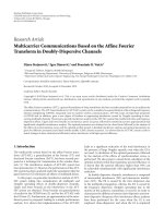
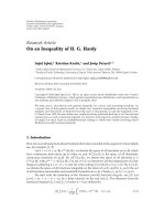
Figure 1 shows a typical adaptive filter setup, where x(n),
d( n), and e(n) are the input, t he desired and the output error
signals, respectively. Here, h(n)istheM
× 1 column vector
of filter coefficients at iteration n.
The generic filter vector update equation at the center of
our analysis is introduced as
h
(

n +1
)
= h
(
n
)
+ μC
(
n
)
X
(
n
)
W
(
n
)
e
(
n
)
,
(1)
where
e
(
n
)
= d

(
n
)
− X
T
(
n
)
h
(
n
)
(2)
is the output error vector. The matrix X(n)istheM
×P input
signal matrix (The parameter P is a positive integer (usually,
but not necessarily P
≤ M)),
h(n)
+
−
y(n)
e(n)
x(n)
d(n)
Figure 1: Prototy pical adaptive filter setup.
X
(
n
)

=
[
x
(
n
)
, x
(
n
− 1
)
, , x
(
n −
(
P
− 1
))]
,
(3)
where x(n)
= [x(n), x(n − 1), , x(n − M +1)]
T
is the input
signal vector, and d(n)isaP
× 1 vector of desired signal
d
(
n
)

=
[
d
(
n
)
, d
(
n
− 1
)
, , d
(
n −
(
P
− 1
))]
T
.
(4)
The desired signal is assumed to be generated from the
following linear model:
d
(
n
)
= X
T
(

n
)
h
t
(
n
)
+ v
(
n
)
,
(5)
where v(n)
= [v(n), v(n − 1), , v(n − (P − 1))]
T
is the
measurement noise vector and assumed to be zero mean,
white, Gaussian, and independent of the input signal, and
h
t
(n) is the unknown filter vector which is time-variant. We
assume that the variation of h
t
(n) is according to the random
walk model [1, 2, 25]
h
t
(
n +1

)
= h
t
(
n
)
+ q
(
n
)
,
(6)
where the sequence of q(n) is an independent and identically
distributed sequence with autocorrelation matrix Q
=
E{q(n)q
T
(n)} and independent of the x(k)forallk and of
the d(k)fork<n.
3. Derivation of SPU Adaptive Filter Algorithms
Different adaptive filter algorithms are established through
the specific choices for the matrices C(n)andW( n)aswellas
for the parameter P.
3.1. The Family of SPU-NLMS Algorithms. From (1), the
generic filter coefficients update equation for P
= 1canbe
stated as
h
(
n +1

)
= h
(
n
)
+ μC
(
n
)
x
(
n
)
W
(
n
)
e
(
n
)
.
(7)
In the adaptive filter algorithms with selective partial
updates, the M
× 1 vector of filter coefficients is partitioned
into K blocks each of length L and in each iteration a
subset of these blocks is updated. For this family of adaptive
filters, the matrices C(n)andW(n) can be obtained from
Table 1,wheretheA(n)matrixistheM

× M diagonal matrix
with the 1 and 0 blocks each of length L on the diagonal
and the positions of 1’s on the diagonal determine which
coefficients should be updated in each iteration. In Ta ble 1,
the parameter L is the length of the block, K is the number
of blocks (K
= (M/L) and is an integer) and N is the number
of blocks to update. Through the specific choices for L, N,
EURASIP Journal on Advances in Sig nal Processing 3
Table 1: Family of adaptive filters with selective partial updates.
Algorithm PLK NC(n) W(n)
Max-NLMS [22]11M 1 A(n)
1
A(n)x(n)
2
N-Max NLMS [16, 23]1 1MN≤ M A(n)
1
x(n)
2
SPU-NLMS [24]1LM/LN≤ K A(n)
1
x(n)
2
SPU-NLMS [17, 18]11MN≤ M A(n)
1
A(n)x(n)
2
SPU-NLMS [17]1LM/L 1 A(n)
1
A(n)x(n)

2
SPU-NLMS [17]1LM/LN≤ K A(n)
1
A(n)x(n)
2
SPU-APA [17] P ≤ MLM/LN≤ K A(n)(X
T
(n)A(n) X(n))
−1
the matrices C(n)andW(n), different SPU-NLMS adaptive
filter algorithms are established.
By partitioning the regressor vector x(n)intoK blocks
each of length L as
x
(
n
)
=

x
T
1
(
n
)
, x
T
2
(
n

)
, , x
T
K
(
n
)

T
,
(8)
the positions of 1 blocks (N blocks and N
≤ K)onthe
diagonal of A(n) matrix for each iteration in the family
of SPU-NLMS adaptive algorithms are determined by the
following procedure:
(1) the
x
i
(n)
2
values are sorted for 1 ≤ i ≤ K;
(2) the i values that determine the positions of 1 blocks
correspond to the N largest values of
x
i
(n)
2
.
3.2. The SPU-APA. The filter vector update equation for

SPU-APA is g iven by [17]
h
F
(
n +1
)
= h
F
(
n
)
+ μX
F
(
n
)

X
T
F
(
n
)
X
F
(
n
)

−1

e
(
n
)
,
(9)
where F
={j
1
, j
2
, , j
N
} denote the indices of the N blocks
out of K blocks that should be updated at every adaptation,
and
X
F
(
n
)
=

X
T
j
1
(
n
)

, X
T
j
2
(
n
)
, , X
T
j
N
(
n
)

T
(10)
is the NL
× P matrix and
X
i
(
n
)
=
[
x
i
(
n

)
, x
i
(
n
− 1
)
, , x
i
(
n
−
(
P
− 1
))]
(11)
is the L
× P matrix. The indices of F are obtained by the
following procedure:
(1) compute the following values for 1
≤ i ≤ K
Tr

X
T
i
(
n
)

X
i
(
n
)

; (12)
(2) the indices of F are correspond to N largest values of
(12).
From (9), the SPU-PRA can also be established when the
adaptation of the filter coefficients is performed only once
every P iterations. Equation (9) can be represented in the
form of full update equation as
h
(
n +1
)
= h
(
n
)
+ μA
(
n
)
X
(
n
)


X
T
(
n
)
A
(
n
)
X
(
n
)

−1
e
(
n
)
,
(13)
where the A(n)matrixistheM
× M diagonal matrix with
the 1 and 0 blocks each of length L on the diagonal and the
positions of 1’s on the diagonal determine which coefficients
should be updated in each iteration. The positions of 1 blocks
(N blocks and N
≤ K) on the diagonal of A(n)matrixfor
each iteration in t he SPU-APA is determined by the indices
of F. Tabl e 1 summarizes the parameters selection for the

establishment of SPU-APA.
4. Tracking Performance Analysis of the Family
of SPU-NLMS and SPU-APA
The steady-state mean square error (MSE) performance of
adaptive filter algorithms can be evaluated from (14):
MSE
= lim
n →∞
E

e
2
(
n
)

.
(14)
In this section, we apply the energy conservation arguments
approach to find the steady-state MSE of the family of SPU-
NLMS and SPU-AP adaptive filter algorithms. By defining
the weight error vector as

h
(
n
)
= h
t
(

n
)
− h
(
n
)
,
(15)
equation (1) can be stated as
h
t
(
n +1
)
− h
(
n +1
)
= h
t
(
n +1
)
− h
(
n
)
− μC
(
n

)
X
(
n
)
W
(
n
)
e
(
n
)
.
(16)
Substituting (6)into(16)yields
h
t
(
n +1
)
− h
(
n +1
)
= h
t
(
n
)

− h
(
n
)
+ q
(
n
)
− μC
(
n
)
X
(
n
)
W
(
n
)
e
(
n
)
.
(17)
4 EURASIP Journal on Advances in Signal Processing
Therefore, (17)canbewrittenas

h

(
n +1
)
=

h
(
n
)
+ q
(
n
)
− μC
(
n
)
X
(
n
)
W
(
n
)
e
(
n
)
.

(18)
By multiplying both sides of (18)fromtheleftbyX
T
(n), we
obtain
e
p
(
n
)
= e
a
(
n
)
− μX
T
(
n
)
C
(
n
)
X
(
n
)
W
(

n
)
e
(
n
)
,
(19)
where e
a
(n)ande
p
(n) are a priori and posteriori error
vectors which are defined as
e
a
(
n
)
= X
T
(
n
)(
h
t
(
n +1
)
− h

(
n
))
= X
T
(
n
)

h
t
(
n
)
+ q
(
n
)
− h
(
n
)

=
X
T
(
n
)



h
(
n
)
+ q
(
n
)

,
e
p
(
n
)
= X
T
(
n
)(
h
t
(
n +1
)
− h
(
n +1
))

= X
T
(
n
)

h
(
n +1
)
.
(20)
Finding e(n)from(19) and substitute it into (18), the
following equality will be established:

h
(
n +1
)
+
(
C
(
n
)
X
(
n
)
W

(
n
))

X
T
(
n
)
C
(
n
)
X
(
n
)
W
(
n
)

−1
e
a
(
n
)
=


h
(
n
)
+ q
(
n
)
+
(
C
(
n
)
X
(
n
)
W
(
n
))
×

X
T
(
n
)
C

(
n
)
X
(
n
)
W
(
n
)

−1
e
p
(
n
)
.
(21)
Taking the Euclidean norm and then expectation from both
sides of (21) and using the random walk model (6), we
obtain after some calculations, that in the nonstationary
environment the following energy equality holds:
E






h
(
n +1
)



2

+ E

e
T
a
(
n
)
W
(
n
)
Z
−1
(
n
)
e
a
(
n

)

=
E





h
(
n
)



2

+ E



q
(
n
)


2


+ E

e
T
p
(
n
)
W
(
n
)
Z
−1
(
n
)
e
p
(
n
)

,
(22)
where Z(n)
= X
T
(n)C(n)X( n) W(n). Using the following
steady-state condition, E{


h(n +1)
2
}=E{

h(n)
2
},yields
E

e
T
a
(
n
)
W
(
n
)
Z
−1
(
n
)
e
a
(
n
)


= E



q
(
n
)


2

+ E

e
T
p
(
n
)
W
(
n
)
Z
−1
(
n
)

e
p
(
n
)

.
(23)
Focusing on the second term of the right-hand side (RHS) of
(23)andusing(19), we obtain
E

e
T
p
(
n
)
W
(
n
)
Z
−1
(
n
)
e
p
(

n
)

=
E

e
T
a
(
n
)
W
(
n
)
Z
−1
(
n
)
e
a
(
n
)

− μE

e

T
a
(
n
)
W
(
n
)
e
(
n
)

−
μE

e
T
(
n
)
Z
T
(
n
)
W
(
n

)
Z
−1
(
n
)
e
a
(
n
)

+ μ
2
E

e
T
(
n
)
Z
T
(
n
)
W
(
n
)

Z
−1
(
n
)
e
(
n
)

.
(24)
By substituting (24) into the second term of RHS of (23)and
eliminating the equal terms from both sides, we have
− μE

e
T
a
(
n
)
W
(
n
)
e
(
n
)


−
μE

e
T
(
n
)
Z
T
(
n
)
W
(
n
)
Z
−1
(
n
)
e
a
(
n
)

+ μ

2
E

e
T
(
n
)
Z
T
(
n
)
W
(
n
)
Z
−1
(
n
)
e
(
n
)

+ E




q
(
n
)


2

=
0.
(25)
From (2)and(5), the relation between the output estimation
error and a priori estimation error vectors is given by
e
(
n
)
= e
a
(
n
)
+ v
(
n
)
.
(26)
Using (26), we obtain

− μE

e
T
a
(
n
)
W
(
n
)
e
a
(
n
)

−
μE

e
T
a
(
n
)
Z
T
(

n
)
W
(
n
)
Z
−1
(
n
)
e
a
(
n
)

+ μ
2
E

e
T
a
(
n
)
Z
T
(

n
)
W
(
n
)
e
a
(
n
)

+ μ
2
E

v
T
(
n
)
Z
T
(
n
)
W
(
n
)

v
(
n
)

+Tr
(
Q
)
= 0.
(27)
The steady-state excess MSE (EMSE) is defined as
EMSE
= lim
n →∞
E

e
2
a
(
n
)

,
(28)
where e
a
(n) is the a priori error signal. To obtain the steady-
state EMSE, we need the following assumption from [12].

At steady-state the input signal and therefore Z(n)and
W(n) are statistically independent of e
a
(n)andmoreover
E
{e
a
(n)e
T
a
(n)}=E{e
2
a
(n)}·S where S ≈ I
P×P
for small μ
and S
≈ (1 · 1
T
) for large μ where 1
T
= [1, 0, ,0]
1×P
.
Based on this, we analyze four parts of (27),
Part I:
E

e
T

a
(
n
)
W
(
n
)
e
a
(
n
)

=
E

e
2
a
(
n
)

Tr
(
SE{W
(
n
)

}
)
. (29)
Part II:
E

e
T
a
(
n
)
Z
T
(
n
)
W
(
n
)
Z
−1
(
n
)
e
a
(
n

)

= E

e
2
a
(
n
)

Tr

SE

Z
T
(
n
)
W
(
n
)
Z
−1
(
n
)


.
(30)
EURASIP Journal on Advances in Sig nal Processing 5
Part III:
E

e
T
a
(
n
)
Z
T
(
n
)
W
(
n
)
e
a
(
n
)

=
E


e
2
a
(
n
)

Tr

SE

Z
T
(
n
)
W
(
n
)

.
(31)
Part IV :
E

v
T
(
n

)
Z
T
(
n
)
W
(
n
)
v
(
n
)

=
σ
2
v
Tr

E

Z
T
(
n
)
W
(

n
)

. (32)
Therefore from (27), the EMSE is given by
E

e
2
a
(
n
)

=
EMSE =
μσ
2
v
Tr

E

Z
T
(
n
)
W
(

n
)

+ μ
−1
Tr
(
Q
)
Tr
(
SE{W
(
n
)
}
)
+Tr
(
SE
{Z
T
(
n
)
W
(
n
)
Z

−1
(
n
)
}
)
− μ Tr
(
SE{Z
T
(
n
)
W
(
n
)
}
)
. (33)
Also from (26), the steady-state MSE can be obtained by
MSE
= EMSE + σ
2
v
.
(34)
From the general expression (33), we will be able to predict
the steady-state MSE of the family of SPU-NLMS, and SPU-
AP adaptive filter algorithms in the nonstationary environ-

ment. Selecting A(n)
= I and the parameters selection
according to Table 1, the tracking performance of NLMS and
APA can also be analyzed.
5. Simulation Results
The theoretical results presented in this paper are confirmed
by several computer simulations for a system identification
setup. The unknown systems have 8 and 16, where the taps
are randomly selected. The input signal x(n)isafirst-order
autoregressive (AR) signal generated by
x
(
n
)
= ρx
(
n − 1
)
+ w
(
n
)
(35)
where w(n) is either a zero mean white Gaussian signal or a
zero mean uniformly distributed random sequence between
−1 and 1. For the Gaussian case, the value of ρ is set to
0.9, generating a highly colored Gaussian signal. For the
uniform distribution case, the value of ρ issetto0.5.The
measurement noise v(n)withσ
2

v
= 10
−3
is added to the noise
free desired signal d(n)
= h
T
t
(n)x( n). The adaptive filter and
the unknown channel are assumed to have the same number
of taps. In all simulations, the simulated learning curves are
obtained by ensemble averaging over 200 independent trials.
Also, the steady-state MSE is obtained by averaging over 500
steady-state samples from 500 independent realizations for
each value of μ for a given algorithm. Also, we assume an
independent and identically distributed sequence for q(n)
with autocorrelation matrix Q
= σ
2
q
· I where σ
2
q
= 0.0025σ
2
v
.
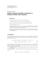
Figures 2–5 show the steady-state MSE of the N-Max
NLMS adaptive algorit hm for M
= 8, and different values for

N as a function of step size in a nonstationary environment.
The step size changes in the stability bound for both colored
Gaussian and uniform distribution input signals. Figure 2
shows the results for N
= 4, and for diffrent input signals.
The theoretical results are from (33). As we can see, the
theoretical values are in good agreement with simulation
results. This agreement is better for uniform input signal.
Figure 3 presents the results for N
= 5. Again, the agreement
is good, specially for uniform input signal. In Figures 4 and
0.1 0.2 0.3 0.4 0.5 0.6 0.7 0.8 0.9 1
−28
−26
−24
−22
−20
(a) N-max NLMS, K
= 8, N = 4, simulation
(b) N-max NLMS, K
= 8, N = 4, theory
(a)
(b)
Input: Guassian AR(1), ρ
= 0.9
MSE (dB)
Step-size (μ)
0.1 0.2 0.3 0.4 0.5 0.6 0.7 0.8 0.9 1
(a) N-max NLMS, K
= 8, N = 4, simulation

(b) N-max NLMS, K
= 8, N = 4, theory
−30
−29
−28
−27
−26
−25
−24
−23
(a)
(b)
MSE (dB)
Step-size (μ)
Input: Uniform AR(1), ρ
= 0.5
Figure 2: Steady-state MSE of N-Max NLMS with M = 8andN =
4 as a function of the s tep size in nonstationary environment for
different input signals.
5, we presented the results for N = 6, and N = 7 respectively.
This figure shows that the derived theoretical expression is
suitable to predict the steady-state MSE of N-Max NLMS
adaptive filter algorithm in nonstationary environment.
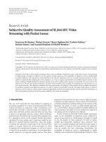
Figures 6–8 show the steady-state MSE of SPU-NLMS
adaptive algorithm wit h M
= 8 as a function of step size
in a nonstationary environment for colored Gaussian and
uniform input signals. We set the number of block (K)to4
and different values for N is chosen in simulations. Figure 6
presents the results for N

= 2andfordifferent input signals.
The good agreement between the theoretical steady-state
MSE and the simulated steady-state MSE is observed. This
fact can be seen in Figures 7 and 8 for N
= 3, and N = 4
respectively .
6 EURASIP Journal on Advances in Signal Processing
0.1 0.2 0.3 0.4 0.5 0.6 0.7 0.8 0.9 1
−28
−26
−24
−22
−20
MSE (dB)
(a) N-max NLMS, K = 8, N = 5, simulation
(b) N-max NLMS, K = 8, N = 5, theory
(a)
(b)
Input: Guassian AR(1), ρ
= 0.9
Step-size (μ)
0.1 0.2 0.3 0.4 0.5 0.6 0.7 0.8 0.9 1
−30
−29
−28
−27
−26
−25
−24
−23

MSE (dB)
(a) N-max NLMS, K = 8, N = 5, simulation
(b) N-max NLMS, K = 8, N = 5, theory
(a)
(b)
Step-size (μ)
Input: Uniform AR(1), ρ
= 0.5
Figure 3: Steady-state MSE of N-Max NLMS with M = 8andN =
5 as a function of the step size in nonstationary environment for
different input signals.
0.1 0.2 0.3 0.4 0.5 0.6 0.7 0.8 0.9 1
−28
−26
−24
−22
−20
Input: Guassian AR(1), ρ
= 0.9
MSE (dB)
(a)
(b)
(a) N-max NLMS, K
= 8, N = 6, simulation
(b) N-max NLMS, K = 8, N = 6, theory
Step-size (μ)
0.1 0.2 0.3 0.4 0.5 0.6 0.7 0.8 0.9 1
−30
−29
−28

−27
−26
−25
−24
−23
(a)
(b)
MSE (dB)
(a) N-max NLMS, K = 8, N = 6, simulation
(b) N-max NLMS, K = 8, N = 6, theory
Step-size (μ)
Input: Uniform AR(1), ρ
= 0.5
Figure 4: Steady-state MSE of N-Max NLMS with M = 8andN =
6 as a function of the step size in nonstationary environment for
different input signals.
0.1 0.2 0.3 0.4 0.5 0.6 0.7 0.8 0.9 1
−28
−26
−24
−22
−20
Input: Guassian AR(1), ρ
= 0.9
MSE (dB)
(a)
(b)
(a) N-max NLMS, K = 8, N = 7, simulation
(b) N-max NLMS, K = 8, N = 7, theory
Step-size (μ)

−28
−26
−24
−22
−20
MSE (dB)
−30
0.1 0.2 0.3 0.4 0.5 0.6 0.7 0.8 0.9 1
(a)
(b)
(a) N-max NLMS, K
= 8, N = 7, simulation
(b) N-max NLMS, K = 8, N = 7, theory
Step-size (μ)
Input: Uniform AR(1), ρ
= 0.5
Figure 5: Steady-state MSE of N-Max NLMS with M = 8andN =
7 as a function of the s tep size in nonstationary environment for
different input signals.
0.1 0.2 0.3 0.4 0.5 0.6 0.7 0.8 0.9 1
−28
−26
−24
−22
−20
Input: Guassian AR(1), ρ
= 0.9
MSE (dB)
(a)
(b)

(a) SPU-NLMS, M
= 8, K = 4, N = 2, simulation
Step-size (μ)
(b) SPU-NLMS, M
= 8, K = 4, N = 2, theory
(a)
(b)
−28
−26
−24
−22
MSE (dB)
−30
0.1 0.2 0.3 0.4 0.5 0.6 0.7 0.8 0.9 1
(a) SPU-NLMS, M
= 8, K = 4, N = 2, simulation
Step-size (μ)
Input: Uniform AR(1), ρ = 0.5
(b) SPU-NLMS, M
= 8, K = 4, N = 2, theory
Figure 6: Steady-state MSE of SPU-NLMS with M = 8, K = 4and
N
= 2 as a function of the step size in nonstationary environment
for different input signals.
EURASIP Journal on Advances in Sig nal Processing 7
0.1 0.2 0.3 0.4 0.5 0.6 0.7 0.8 0.9 1
−28
−26
−24
−22

−20
MSE (dB)
(a)
(b)
Input: Guassian AR(1), ρ
= 0.9
(a) SPU-NLMS, M
= 8, K = 4, N = 3, simulation
(b) SPU-NLMS, M = 8, K = 4, N = 3, theor y
Step-size (μ)
0.1 0.2 0.3 0.4 0.5 0.6 0.7 0.8 0.9 1
−30
−29
−28
−27
−26
−25
−24
−23
MSE (dB)
(a)
(b)
(a) SPU-NLMS, M
= 8, K = 4, N = 3, simulation
(b) SPU-NLMS, M = 8, K = 4, N = 3, theor y
Step-size (μ)
Input: Uniform AR(1), ρ
= 0.5
Figure 7: Steady-state MSE of SPU-NLMS with M = 8, K = 4and
N

= 3 as a function of the step size in nonstationary environment
for different input signals.
0.1 0.2 0.3 0.4 0.5 0.6 0.7 0.8 0.9 1
−28
−26
−24
−22
−20
Input: Guassian AR(1), ρ
= 0.9
MSE (dB)
(a)
(b)
(a) SPU-NLMS, M
= 8, K = 4, N = 4, simulation
(b) SPU-NLMS, M
= 8, K = 4, N = 4, theory
Step-size (μ)
−28
−26
−24
−22
−20
MSE (dB)
−30
0.1 0.2 0.3 0.4 0.5 0.6 0.7 0.8 0.9 1
(a)
(b)
(a) SPU-NLMS, M
= 8, K = 4, N = 4, simulation

(b) SPU-NLMS, M = 8, K = 4, N = 4, theor y
Step-size (μ)
Input: Uniform AR(1), ρ
= 0.5
Figure 8: Steady-state MSE of SPU-NLMS with M = 8, K = 4and
N
= 4 as a function of the step size in nonstationary environment
for different input signals.
0 0.1 0.2 0.3 0.4 0.5 0.6 0.7 0.8 0.9 1
−28
−27
−26
−25
−24
−23
−22
Input: Guassian AR(1), ρ
= 0.9
(a) SPU-APA, M
= 8, P = 4, K = 4, N = 2, simulation
(b) SPU-APA, M
= 8, P = 4, K = 4, N = 2, theory
MSE (dB)
(a)
(b)
Step-size (μ)
0 0.1 0.2 0.3 0.4 0.5 0.6 0.7 0.8 0.9 1
−30
−29
−28

−27
−26
(a) SPU-APA, M
= 8, P = 4, K = 4, N = 2, simulation
(b) SPU-APA, M
= 8, P = 4, K = 4, N = 2, theory
MSE (dB)
(a)
(b)
Step-size (μ)
Input: Uniform AR(1), ρ
= 0.5
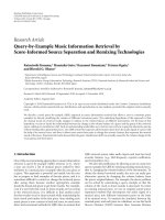
Figure 9: Steady-state MSE of SPU-APA with M = 8, P = 4,
K
= 4andN = 2 as a function of the step size in nonstationar y
environment for different input signals.
0 0.1 0.2 0.3 0.4 0.5 0.6 0.7 0.8 0.9 1
−29
−28
−27
−26
−25
−24
MSE (dB)
(a)
(b)
Input: Guassian AR(1), ρ = 0.9
(a) SPU-APA, M
= 8, P = 4, K = 4, N = 3, simulation
(b) SPU-APA, M

= 8, P = 4, K = 4, N = 3, theory
Step-size (μ)
0 0.1 0.2 0.3 0.4 0.5 0.6 0.7 0.8 0.9 1
−29.5
−29
−28.5
−28
−27.5
−27
−26.5
MSE (dB)
(a)
(b)
(a) SPU-APA, M = 8, P = 4, K = 4, N = 3, simulation
(b) SPU-APA, M
= 8, P = 4, K = 4, N = 3, theory
Step-size (μ)
Input: Uniform AR(1), ρ
= 0.5
Figure 10: Steady-state MSE of SPU-APA with M = 8, P = 4,
K
= 4andN = 3 as a function of the step size in nonstationar y
environment for different input signals.
8 EURASIP Journal on Advances in Signal Processing
MSE (dB)
(a)
(b)
−29
−28
−27

−26
−25
0 0.1 0.2 0.3 0.4 0.5 0.6 0.7 0.8 0.9 1
Input: Guassian AR(1), ρ
= 0.9
(a) SPU-APA, M = 8, P = 4, K = 4, N = 4, simulation
(b) SPU-APA, M
= 8, P = 4, K = 4, N = 4, theory
Step-size (μ)
0 0.1 0.2 0.3 0.4 0.5 0.6 0.7 0.8 0.9 1
−30
−29
−28
−27
−26
MSE (dB)
(a)
(b)
(a) SPU-APA, M = 8, P = 4, K = 4, N = 4, simulation
(b) SPU-APA, M = 8, P = 4, K = 4, N = 4, theory
Step-size (μ)
Input: Uniform AR(1), ρ
= 0.5
Figure 11: Steady-state MSE of SPU-APA with M = 8, P = 4,
K
= 4andN = 4 as a function of the step size in nonstationary
environment for different input signals.
0 500 1000 1500 2000 2500 3000
−30
−25

−20
−15
−10
−5
0
5
10
15
Iteration
10 log(MSE) dB
(a)
(a) N-max NLMS, K
= 8, N = 4, μ = 0.2
(b) N-max NLMS, K = 8, N = 4, μ = 0.4
(c) N-max NLMS, K
= 8, N = 4, μ = 0.6
Theoretical
Input: Guassian AR(1), ρ
= 0.9
(b)
(c)
Figure 12: Learning curves of N-Max NLMS with M = 8andN =
4anddifferent values of the step size for colored Gaussian i nput
signal.
0 500 1000 1500 2000 2500 3000
−30
−25
−20
−15
−10

−5
0
5
10
15
Iteration
10 log(MSE) dB
(a)
Theoretical
(b)
(c)
Input: Guassian AR(1), μ
= 0.9
(a) SPU-NLMS, M
= 8, K = 4, N = 4, μ = 0.1
(b) SPU-NLMS, M
= 8, K = 4, N = 3, μ = 0.1
(c) SPU-NLMS, M
= 8, K = 4, N = 2, μ = 0.1
Figure 13: Learning curves of SPU-NLMS with M = 8, K = 4, and
N
= 2, 3, 4 for colored Gaussian input signal.
0 500 1000 1500 2000 2500 3000
−30
−25
−20
−15
−10
−5
0

5
10
15
Iteration
10 log(MSE) dB
(a)
Theoretical
Input: Guassian AR(1), ρ
= 0.9
(b)
(c)
(a) SPU-NLMS, M
= 8, K = 4, N = 3, μ = 0.1, σ
2
q
= 0.0025σ
2
v
(b) SPU-NLMS, M = 8, K = 4, N = 3, μ = 0.1, σ
2
q
= 0.025σ
2
v
(c) SPU-NLMS, M = 8, K = 4, N = 3, μ = 0.1, σ
2
q
= 0.0015σ
2
v

Figure 14: Learning curves of SPU-NLMS with M = 8, K = 4
and N
= 3fordifferent degree o f nonstationary and for colored
Gaussian input signal.
EURASIP Journal on Advances in Sig nal Processing 9
−5
−25
−20
−15
−10
(a) SPU-NLMS, M = 16, K = 4, N = 2, simulation
(b) SPU-NLMS, M = 16, K = 4, N = 2, theor y
0 0.1 0.2 0.3 0.4 0.5 0.6 0.7 0.8 0.9 1
MSE (dB)
(a)
(b)
Input: Guassian AR(1), ρ = 0.9
Step-size (μ)
−25
−20
−15
−10
−30
(a) SPU-NLMS, M = 16, K = 4, N = 2, simulation
(b) SPU-NLMS, M
= 16, K = 4, N = 2, theory
0 0.1 0.2 0.3 0.4 0.5 0.6 0.7 0.8 0.9 1
MSE (dB)
(a)
(b)

Step-size (μ)
Input: Uniform AR(1), ρ
= 0.5
Figure 15: Steady-state MSE of SPU-NLMS with M = 16, K =
4andN = 2 as a function of the step s ize in nonstationar y
environment for different input signals.
0 0.1 0.2 0.3 0.4 0.5 0.6 0.7 0.8 0.9 1
MSE (dB)
(a)
(b)
Input: Guassian AR(1), ρ
= 0.9
−25
−20
−15
−10
(a) SPU-NLMS, M = 16, K = 4, N = 3, simulation
(b) SPU-NLMS, M = 16, K = 4, N = 3, theory
Step-size (μ)
MSE (dB)
(a)
(b)
−28
−26
−24
−22
−20
−18
−16
−14

0 0.1 0.2 0.3 0.4 0.5 0.6 0.7 0.8 0.9 1
(a) SPU-NLMS, M = 16, K = 4, N = 3, simulation
(b) SPU-NLMS, M = 16, K = 4, N = 3, theory
Step-size (μ)
Input: Uniform AR(1), ρ
= 0.5
Figure 16: Steady-state MSE of SPU-NLMS with M = 16, K =
4, and N = 3 as a function of the step size in nonstationary
environment for different input signals.
0 0.1 0.2 0.3 0.4 0.5 0.6 0.7 0.8 0.9 1
MSE (dB)
(a)
(b)
−24
−22
−20
−18
−16
−14
−12
(a) SPU-NLMS, M
= 16, K = 4, N = 4, simulation
(b) SPU-NLMS, M
= 16, K = 4, N = 4, theory
Input: Guassian AR(1), ρ
= 0.9
Step-size (μ)
0 0.1 0.2 0.3 0.4 0.5 0.6 0.7 0.8 0.9 1
MSE (dB)
(a)

(b)
−28
−26
−24
−22
−20
−18
−16
−14
(a) SPU-NLMS, M
= 16, K = 4, N = 4, simulation
(b) SPU-NLMS, M
= 16, K = 4, N = 4, theory
Step-size (μ)
Input: Uniform AR(1), ρ
= 0.5
Figure 17: Steady-state MSE of SPU-NLMS with M = 16, K =
4, and N = 4 as a function of the step size in nonstationary
environment for different input signals.
Figures 9–11 show the steady-state MSE of SPU-APA as a
function of step size for M
= 8, and different input signals.
The parameters K,andP were set to 4, and the step size
changesfrom0.05to1.Different values for N have been
used in simulations. Figure 9 sho ws the results for N
= 2.
Simulation results show good agreement for both colored
and uniform input signals. In Figure 10, we set the parameter
N to 3. Again good agreement can be seen especially for
uniform input signal. Finally, Figure 11 shows the results for

N
= 4. As we can see, the presented theoretical relation is
suitable to predict the steady-state MSE.
Figures 12–14 show the simulated learning curves of
SPU adaptive filter algorithms for different parameters values
and for colored Gaussian input signal. Figure 12 presents
the learning curves for N-Max NLMS algorithm with M
=
8, N = 4anddifferent values for the step size. Also,
the theoretical steady-state MSE was calculated based on
(33) and compared with simulated steady-state MSE. As we
can see the theoretical values are in good agreement with
simulation results. Figure 13 shows the learning curves of
SPU-NLMS algorithm with M
= 8, K = 4, and N = 2, 3, 4.
Also, the step size was set to 0.1. Again the theoretical values
of the steady-state MSE has been shown in this figure. Again
good agreement is observed. In Figure 14, the learning curves
of SPU-NLMS with M
= 8, K = 4, and N = 3, have
been presented for different values of σ
2
q
.Thedegreeof
nonstationary changes by selecting different values for σ
2
q
.As
we can see, for the large values of σ
2

q
, the agreement between
10 EURASIP Journal on Advances in Signal Processing
0 0.1 0.2 0.3 0.4 0.5 0.6 0.7 0.8 0.9 1
MSE (dB)
−27
−26
−25
−24
−23
−22
−21
(a)
(b)
(a) SPU-APA, M
= 16, P = 4, K = 4, N = 3, simulation
(b) SPU-APA, M = 16, P = 4, K = 4, N = 3, theory
Input: Guassian AR(1), ρ
= 0.9
Step-size (μ)
0 0.1 0.2 0.3 0.4 0.5 0.6 0.7 0.8 0.9 1
MSE (dB)
−29
−28
−27
−26
−25
−24
−23
(a)

(b)
(a) SPU-APA, M
= 16, P = 4, K = 4, N = 3, simulation
(b) SPU-APA, M
= 16, P = 4, K = 4, N = 3, theory
Step-size (μ)
Input: Uniform AR(1), ρ = 0.5
Figure 18: Steady-state MSE of SPU-APA with M = 16, P = 4, K = 4, and N = 3 as a function of the step size in nonstationary environment
for different input signals.
0 0.1 0.2 0.3 0.4 0.5 0.6 0.7 0.8 0.9 1
MSE (dB)
−28
−26
−24
−22
−20
(a)
(b)
(a) SPU-APA, M
= 16, P = 4, K = 4, N = 4, simulation
(b) SPU-APA, M
= 16, P = 4, K = 4, N = 4, theory
Input: Guassian AR(1), ρ
= 0.9
Step-size (μ)
0 0.1 0.2 0.3 0.4 0.5 0.6 0.7 0.8 0.9 1
MSE (dB)
−29
−28
−27

−26
−25
−24
−23
(a)
(b)
(a) SPU-APA, M
= 16, P = 4, K = 4, N = 4, simulation
(b) SPU-APA, M
= 16, P = 4, K = 4, N = 4, theory
Step-size (μ)
Input: Uniform AR(1), ρ
= 0.5
Figure 19: Steady-state MSE of SPU-APA with M = 16, P = 4, K = 4, and N = 4 as a function of the step size in nonstationary environment
for different input signals.
simulated steady-state MSE and theoretical steady-state MSE
is deviated.
Figures 15–17 show the steady-state MSE of SPU-NLMS
adaptive algorithm with M
= 16 as a function of step size
in a nonstationary environment for colored Gaussian and
uniform input signals. We set the number of blocks (K)
to 4 and different values for N arechoseninsimulations.
Figure 15 presents the results for N
= 2andfordifferent
input signals. The good agreement between the theoretical
steady-state MSE and the simulated steady-state MSE is
observed. In Figures 16 and 17,wepresentedtheresultsfor
N
= 3, and 4. Simulation results show good agreement for

both colored and uniform input signals.
Figures 18 and 19 show the steady-state MSE of SPU-
APA as a function of step size for M
= 16, and different
input signals. The parameters K,andP weresetto4,and
the step size changes from 0.04 to 1. Different values for N
have been used in simulations. Figure 18 shows the results
for N
= 3. In Figure 19,theparameterN was set to 4.
Again good agreement can be seen for both input signals.
The simulation results show that the agreement is deviated
for M
= 16.
6. Summary and Conclusions
We presented a general framework for tracking performance
analysis of the family of SPU-NLMS adaptive filter algo-
rithms in nonstationary environment. Using the general
expression and for the parameter values in Table 1,themean
square performances of Max-NLMS, N-Max NLMS, the
various t ypes of SPU-NLMS, and SPU-APA can be analyzed
in a unified way. We demonstrated the usefulness of the
presented analysis through several simulation results.
References
[1] B. Widrow and S. D. Stearns, Adaptive Signal Processing,
Prentice H all, Englewood Cliffs, NJ, USA, 1985.
[2] S. Haykin, Adaptive Filter Theory, Prentice Hall, Englewood
Cliffs, NJ, USA, 4th edition, 2002.
EURASIP Journal on Advances in Signal Processing 11
[3] A.H.Sayed,Adaptive Filters, John Wiley & Sons, New York,
NY, USA, 2008.

[4] B.Widrow,J.M.McCool,M.G.Larimore,andC.R.Johnson
Jr., “Stationary and nonstationr y learning characteristics
of the LMS adaptive filter,” Proceedings of the IEEE, vol. 64, no.
8, pp. 1151–1162, 1976.
[5]N.J.Bershad,F.A.Reed,P.L.Feintuch,andB.Fisher,
“Tracking charcteristics of the LMS adaptive line enhancer:
response to a linear chrip sig nal in noise,” IEEE Transactions
on Acoustics, Speech, and Signal Processing,vol.28,no.5,pp.
504–516, 1980.
[6] S. Marcos and O. Macchi, “Tracking capability of the least
mean square algorithm: application to an asynchronous echo
canceller,” IEEE Transactions on Acoustics, Speech, and Signal
Processing, vol. 35, no. 11, pp. 1570–1578, 1987.
[7] E. Eweda, “Analysis and design of a signed regressor LMS
algorithm for stationary and nonstationary adaptive filtering
with correlated Gaussian data,” IEEE Transactions on Circuits
and Systems, vol. 37, no. 11, pp. 1367–1374, 1990.
[8] E. Eweda, “Optimum step size of sign algorithm for non-
stationary adaptive filtering,” IEEE Transactions on Acoustics,
Speech, and Signal Processing, vol. 38, no. 11, pp. 1897–1901,
1990.
[9] E. Eweda, “Comparison of RLS, LMS, and sign a lgorithms for
tracking randomly time-varying channels,” IEEE Transactions
on Signal Processing, vol. 42, no. 11, pp. 2937–2944, 1994.
[10] N. R. Yousef and A. H. Sayed, “Steady-state and tracking
analyses of the sig n algorithm without the explicit use of the
independence assumption,” IEEE Signal Processing Letters,vol.
7, no. 11, pp. 307–309, 2000.
[11] N. R. Yousef and A. H. Sayed, “A unified approach to the
steady-state and tracking analyses of adaptive filters,” IEEE

Transactions on Signal Processing, vol. 49, no. 2, pp. 314–324,
2001.
[12] H C. Shin and A. H. Sayed, “Mean-square performance of a
family of affine projection algorithms,” IEEE Transactions on
Signal Processing, vol. 52, no. 1, pp. 90–102, 2004.
[13] A. H. Sayed and M. Rupp, “A time-domain feedback analysis
of adaptive algorithms v ia the small gain theorem,” in
Advanced Signal Processing Algorithms, vol. 2563 of Proceedings
of SPIE, San Diego, Calif, USA, 1995.
[14] M. Rupp and A. H. Sayed, “A time-domain feedback analysis
of filteredor adaptive gradient algorithms,” IEEE Transactions
on Signal Processing, vol. 44, no. 6, pp. 1428–1439, 1996.
[15]H C.Shin,W J.Song,andA.H.Sayed,“Mean-square
performance of data-reusing adaptive algorithms,” IEEE Signal
Processing Letters, vol. 12, no. 12, pp. 851–854, 2005.
[16] T. Aboulnasr and K. Mayyas, “Complexity reduction of
the NLMS algorithm via s elective coefficient update,” IEEE
Transactions on Signal Processing, vol. 47, no. 5, pp. 1421–1424,
1999.
[17] K. Do
˘
ganc¸ay, “Adaptive filtering algorithms with selective
partial updates,” IEEE Transactions on Circuits and Systems II:
Analog and Digital Signal Processing, vol. 48, no. 8, pp. 762–
769, 2001.
[18]S.Werner,M.L.R.deCampos,andP.S.R.Diniz,“Partial-
Update NLMS Algorithms with Data-Selective Updating,”
IEEE Transactions on Signal Processing, vol. 52, no. 4, pp. 938–
949, 2004.
[19] M. S. E. Abadi and J. H. Husøy, “Mean-square performance

of the family of adaptive filters with selective partial updates,”
Signal Processing, vol. 88, no. 8, pp. 2008–2018, 2008.
[20] K. Do
˘
ganc
¸ay, Partial-Update Adaptive Signal Processing, Design
Analysis and implementation, Academic Press, New York, NY,
USA, 2009.
[21] A. W.H. Khong and P. A. Na ylor, “Selective-tap adaptive
filtering with performance analysis for identification of time-
varying systems,” IEEE Transactions on Audio, Speech and
Language Processing, vol. 15, no. 5, pp. 1681–1695, 2007.
[22] S. C. Douglas, “Analysis and implementation of the max-
NLMS adaptive filter,” in Proceedings of the 29th Conference on
Signals, Systems, and Computers, pp. 659–663, Pacific Grove,
Calif, USA, October 1995.
[23] T. Aboulnasr and K. Mayyas, “Selective coefficient update of
gradient-based adaptive algorithms,” in Proceedings of the 1997
IEEE International Conference on Acoustics, Speech, and Signal
Processing (ICASSP ’97), pp. 1929–1932, Munich, Germany,
April 1997.
[24] T. Sc hertler, “Selective block update of NLMS type algo-
rithms,” in Proceedings of the IEEE International Conference on
Acoustics, Speech and Sig nal Processing (ICASSP ’98), pp. 1717–
1720, Seattle, Wash, USA, May 1998.
[25] A. H. Sayed, Fundamentals of Adaptive Filtering,JohnWiley&
Sons, New York, NY, USA, 2003.