Báo cáo hóa học: " Research Article Formal Methods for Scheduling of Latency-Insensitive Designs" pptx

Hindawi Publishing Corporation
EURASIP Journal on Embedded Systems
Volume 2007, Article ID 39161, 16 pages
doi:10.1155/2007/39161
Research Article
Formal Methods for Scheduling of Latency-Insensitive Designs
Julien Boucaron, Robert de Simone, and Jean-Vivien Millo
Aoste project-team, INRIA Sophia-Antipolis, 2004 rouye des Iucioles, BP 93, 06902 Sophia Antipolis Cedex, France
Received 1 July 2006; Revised 23 January 2007; Accepted 11 May 2007
Recommended by Jean-Pierre Talpin
Latency-insensitive design (LID) theory was invented to deal with SoC timing closure issues, by allowing arbitrary fixed integer la-
tencies on long global wires. Latencies are coped with using a resynchronization protocol that performs dynamic scheduling of data
transportation. Functional behavior is preserved. This dynamic scheduling is implemented using specific synchronous hardware
elements: relay-stations (RS)andshell-wrappers (SW).OurfirstgoalistoprovideaformalmodelingofRS and SW,thatcanbe
then formally verified. As turns out, resulting behavior is k-periodic, thus amenable to static scheduling. Our second goal is to pro-
vide formal hardware modeling here also. It initially performs throughput equalization, adding integer latencies wherever possible;
residual cases require introduction of fractional registers (FRs) at specific locations. Benchmark results are presented, run on our
Kpassa tool implementation.
Copyright © 2007 Julien Boucaron et al. This is an open access article distributed under the Creative Commons Attribution
License, which permits unrestr icted use, distr ibution, and reproduction in any medium, provided the original work is properly
cited.
1. INTRODUCTION
Long wire interconnect latencies induce time-closure diffi-
culties in modern SoC designs, with propagation of signals
across the die in a single clock cycle being problematic. The
theory of latency-insensitive design (LID), proposed origi-
nallybyCarlonietal.[1, 2], offers solutions for this issue.
This theory can roughly be described as such: an initial fully
synchronous reference specification is first desynchronized as
an asynchronous network of synchronous block components
(a GALS system); it is then resynchronized, but this time with

proper interconnect mechanisms allowing specified (integer-
time) latencies.
Interconnects consist of fixed-sized lines of so-called
relay-stations. These relay-stations, together with shell-
wrapper around the synchronous Pearl IP blocks, are in
charge of managing the signal value fl ows. With their help
proper regulation of the signal trafficisperformed.Compu-
tation blocks may be temporarily paused at times, either be-
cause of input signal unavailability, or because of the inabil-
ity of the rest of the networks to store their outputs if they
were produced. This latter issue stems from the limitation
of fixed-size buffering capacity of the interconnects (relay-
station lines).
Since their invention, relay-stations have been a subject of
attention for a number of research groups. Extensive model-
ing, characterization, and analysis were provided in [3–5].
We mentioned b efore that the process of introducing la-
tencies into synchronous networks introduced, at least con-
ceptually, an intermediate asynchronous representation. This
corresponds to marked graphs [6], a well-studied model of
computation in the literature. The main property of marked
graph is the absence of choice which matches with the ab-
sence of control in LID.
Marked graphs with latencies were also considered under
the name of weighted marked graphs (WMG) [7]. We will re-
duce WMGs to ordinary marked graphs by introducing new
intermediate transportation nodes (TN), akin to the previous
computation nodes (CN) but with a single input and out-
put link.InfactLID systems can be thought of as WMGs
with buffers of capacity 2 (exactly) on link between com-

putation and/or transportation nodes.Therelay-stations and
shell-wrappers are an operational means to implement the
corresponding flow-control and congestion avoidance mech-
anisms with explicit synchronous mechanisms.
The general theory of WMG provides many useful in-
sights. In particular, it teaches us that there exists static repet-
itive scheduling for such computational behaviors [8,
9].
Such static k-periodic schedulings have been applied to soft-
ware pipelining problems [10, 11], and later SoC LID design
problems in [12]. But these solutions pay in general little at-
tention to the form of buffering elements that are holding
values in the scheduled system, and their adequacy for hard-
ware circuit representation. We will try to provide a solution
2 EURASIP Journal on Embedded Systems
that “perfectly” equalizes latencies over reconvergent paths,
so that tokens always arrive simultaneously at the compu-
tation node. Sadly, this cannot always be done by inserting
an integer number of latency under the form of additional
transportation sections. One sometimes needs to hold back
token for one step discriminatingly and sometimes does not.
We provide our solution here under the form of fractional
registers (FR), that may hold back values according to an (in-
put) regular pattern that fits the need for flow-control. Again
we contribute explicit synchronous descriptions of such ele-
ments, with correctness properties. We also rely deeply on a
syntax for schedule representation, borrowed from the the-
ory of N-synchronous processes [13].
Explicit static scheduling that uses predictable syn-
chronous elements is desira ble for a number of issues. It al-

lows a posteriori precise redimensioning of glue buffering
mechanisms between local synchronous elements to allow
the system to work, and this without affecting the compo-
nents themselves. Finally, the extra virtual latencies intro-
duced by equalization could be absorbed by the local compu-
tation times of CN, to resynthesize them under relaxed tim-
ing constraints.
We built a prototy pe tool for equalization of latencies
and fractional registers insertion. It uses a number of elabo-
rated graph-theoretical and linear-programming algorithms.
We will briefly describe this implementation.
Contributions
Our first contribution is to provide a formal description
of rela y-stations and shell-wrappers as synchronous elements
[14], something that was never done before in our knowledge
(the closest effort being [15]). We introduce local correctness
properties that can be easily model-checked; these generic lo-
cal properties, when combined, ensure the global property of
the network.
We introduce the equalization process to statically sched-
ule an LID specification: slowing down “too fast” cycles while
maintaining the original throughput of the LID specification.
The goal is to simplify the LID protocol.
But rational difference of rates may still occur after equal-
ization process, we solve it by adding fractional registers (FR),
that may hold back values according to a regular pattern that
fits the need for flow-control.
We introduce a new class of smooth schedules that op-
timally minimizes the number of FRs used on a statically
scheduled LID design.

Article outline
In the next section we provide some definitional and nota-
tional background on various models of computations in-
volved in our modeling framework, together with an explicit
representation of periodic schedules and firing instants; with
this we can state historical results on k-periodic scheduling
of WMGs.InSection 3, we provide the synchronous reac-
tive representation of relay-stations and shell-wrappers, show
their use in dynamic scheduling of latency-insensitive design,
and describe several formal local correctness properties that
help with the global correctness property of the full network.
Statically scheduled LID systems are tackled in Section 4;we
describe an algorithm to build a statical ly scheduled LID,
possibly adding extra virtual integer latencies and even frac-
tional registers. We provide a running example to highlight
potential difficulties. We also present benchmarks result of
a prototype tool which implements the previous algorithms
and their variations. We conclude with considerations on po-
tential further topics.
2. MODELING FRAMEWORK
2.1. Computation nets
We start from a very general definition, describing what is
common of all our models.
Definition 1 (computation network scheme). A computation
networkscheme(CNS)isagraphwhoseverticesarecalled
Computation Nodes, and whose arcs are called links. We also
allow arcs without a source vertex, called input links, or with-
out target vertex, called output links.
An instance of a CNS is depicted on Figure 1(a).
The intention is that computation nodes perform compu-

tations by consuming a data on each of its incoming links, and
producing as a result a new data on each of its outgoing links.
The occurrence of a computation thus only depends on
data presence and not their actual values, so that data can be
safely abstrac ted as tokens.ACNS is choice free.
In the sequel we will often consider the special case where
the CNS forms a strongly connected graph, unless specified
explicitly.
This simple model leaves out the most important features
that are mandatory to define its operational semantics under
the form of behavioral firing rules. Such features are
(i) the initialization setting (where do tokens reside ini-
tially),
(ii) the nature of links (combinatorial wires, simple regis-
ters, bounded or unbounded place,etc.),
(iii) and the nature of time (synchronous, with compu-
tations firing simultaneously as soon as they can, or
asynchronous, w ith distinct computations firing inde-
pendently).
Setting up choices in these features provides distinct models
of computation.
2.2. Synchronous/asynchronous versions
Definition 2. A synchronous reactive net (S/R net) is a CNS
where time is synchronous: all computation nodes fire simul-
taneously. In addition links are either (memoryless) combi-
natorial wires or simple registers, and all such registers ini-
tially hold a token.
The S/R model conforms to synchronous digital circuits
or (single-clock) synchronous reactive formalisms [16]. The
network operates “at full speed”: there is always a value

present in each register, so that CN operates at each instant.
Julien Boucaron et al. 3
(a)
11
1
3
(b)
(c)
00

1

1

01(0

1101)
∗
011100(11010)
∗
110011(01011)
∗
100110(10110)
∗
111001(10101)
∗
110011(01011)
∗
(d)
Figure 1: (a) An example of CNS (with rectangular computation

nodes), (b) a corresponding WMG with latency features and to-
ken information, (c) an SMG/LID w ith explicit (rectangular) trans-
portation nodes and (oval) places/relay-stations, dividing arcs ac-
cording to latencies, (d) an LID with explicit schedules.
As a result, they consume all values (from registers and
through wires), and replace them again w ith new values pro-
duced in each register . The system is causal if and only if there
is at least one register along each cycle in the graph. Causal
S/R nets are well behaved in the sense that their semantics is
well founded.
Definition 3. A marked graph is a CNS where time is asyn-
chronous: computations are performed independently, pro-
vided they find enough tokens in their incoming links; links
have a place holding a number of tokens; in other words,
marked graphs form a subclass of Petri Nets. The initial mark-
ing of the graph is the number of tokens held in each place.
In addition a marked graph is said to be of capacity k if each
place can hold no more than k tokens.
There is a simple way to encode marked graphs with ca-
pacity as mar ked graphs with unbounded capacity: this re-
quires to add a reverse link for each existing one, which con-
tains initially a number of tokens equal to the difference be-
tween the capacity and the initial marking of the original link.
It was proved that a strongly connected marked graph is
live (each computation can always be fired in the future) if
and only if there is at least one token in every cycle in the
graph [6]. Also, the total number of tokens in a cycle is an
invariant, so strongly connected marked graphs are k-safe for
a given capacity k.
Under proper initial conditions S/R nets and marked

graphs behave essentially the same, with S/R systems per-
forming all computations simultaneously “at full rate,” while
similar computations are now performed independently in
time in marked g raph.
Definition 4. A sy nchronous marked graph (SMG) is a marked
graph with an ASAP (as soon a s possible) semantics: each com-
putation node (transition) that may fire due to the availabil-
ity of it input tokens immediately does so (for the current
instant).
SMGs and the ASAP firing rule are underlying the works
of [8, 9], even though the y are not explicitly given name
there.
Figure 1(c) shows a synchronous marked graph. Note that
SMGs depart from S/R models: here all tokens are not always
available.
2.3. Adding latencies and time durations
We now add latency information to indicate transportation
or computation durations. These latencies will be all along
constant integers (provided from “outside”).
Definition 5. A weighted marked graph (WMG) is a CNS with
(constant integer) latency labels on links. This number indi-
cates the time spent while performing the corresponding to-
ken transportation along the link.
We avoid computation latencies on CNs, which can be
encoded as transportation latencies on links by splitting the
actual CN into a begin/end
CN. Since latencies are global
time durations, the relevant semantics which take them into
account is necessarily ASAP. The system dynamics also im-
poses that one should record at any instant “how far” each

token is currently in its tr avel. This can be modeled by an
age stamp on token, or by expanding the WMG links with
new transportation nodes (TN) to divide them into as many
sections of unit latency. TNs are akin to CNs, with the partic-
ularity that they have unique source and target links. This ex-
pansion amounts to reducing WMGs to (much larger) plain
SMGs. Depending on the concern, the compact or the ex-
panded form may be preferred.
Figure 1(b) displays a weighted marked graph obtained by
adding latencies to Figure 1(a), which can be expanded into
the SMG of Figure 1(c).
For correctness matters there, still should be at least one
token along each cycle in the graph, and less token on a link
than its prescribed latency. This corresponds to the correct-
ness required on the expanded SMG form.
4 EURASIP Journal on Embedded Systems
Definition 6. A latency-insensitive design (LID) is a WMG
where the expanded SMG obtained as above uses places of
capacity 2 in between CNs and TNs.
This definition reads much differently than the original
one in [2]. This comes partly from an important concern of
the authors then, which is to provide a description built with
basic components ( named relay-stations and shell-wrappers)
that can easily be implemented in hardware. Next Section 3
provides a formal representation of relay-stations and shell-
wrappers, together with their properties.
Summar y
CNs lead themselves quite naturally to both synchronous and
asynchronous interpretations. Under some easily expected
initial conditions, these variants can be shown to provide the

same input/output behaviors. With explicit latencies to be
considered in computation and data transportation this re-
mains true, even if congestion mechanisms may be needed
in case of bounded resources. The equivalence in the order-
ing of event between a synchronous circuit and an LID circuit
is shown in [1], and equivalence between an MG and an S/R
design is show n in [17].
2.4. Periodic behaviors, throughput,
and explicit schedules
We now provide the definitions and classical results needed
to justify the existence of static scheduling. This will be used
mostly in Section 4, when we develop our formal modeling
for such scheduling using again synchronous hardware ele-
ments.
Definition 7 (rate, throughput and critical cycles). Let G be a
WMG graph, and C a cycle in this graph.
The rate R of the cycle C is equal to T/L,whereT is the
number of tokens in the cycle, and L is the sum of latencies
of the arcs of this given cycle.
The throughput of the graph is defined as the minimum
rate among all cycles of the graph.
Acycleiscalledcritical if its r ate is equal to the throughput
of the graph.
A classical result states that, provided simple st ructural
correctness conditions, a strongly connected WMG runs un-
der an ultimately k-periodic schedule, with the throughput
of the graph [8, 9]. We borrow notation from the theory of
N-synchronous processes
[13] to represent these notions for-
mally, as explicit analysis and design objects.

Definition 8 (schedules, periodic words, k-periodic sched-
ules). A pre-schedule for a CNS is a function Sched: N
→ w
N
assigning an infinite binary word w
N
∈{0, 1}
ω
to every com-
putation node and transportation node N of the graph. Node
N is activated (or triggered, or fired, or run) at global instant i
if and only if w
N
(i) = 1, where w(i) is the ith letter of word w.
A preschedule is a schedule if the allocated activity in-
stants are in accordance with the token distribution (the
lengthy but straig htforward definition is left to the reader).
Furthermore, the schedule is called ASAP if it activates a
node N whenever all its input tokens have arrived (accord-
ing to the global timing).
An infinite binary word w
∈{0, 1}
ω
is called ultimately
periodic: if it is of the form u
· (v)
ω
where u and v ∈{0, 1}

,

u represents the initialization phase, and v the periodic one.
The length of v is noted
|v| and called its period.The
number of occurrences of 1 s in v is denoted by
|v|
1
and
called its periodicity.Therate R of an ultimately periodic
word w is defined as
|v|
1
/|v|.
Ascheduleiscalledk-periodic whenever for all N, w
N
is
a periodic word.
Thus a schedule is constructed by simulating the CNS ac-
cording to its (deterministic) ASAP firing r ule.
Furthermore, it has been shown in [9] that the length of
the stationary periodic phase (called period) can be com-
puted based on the structure of the graph and the (static)
latencies of cycles: for a critical strongly connected compo-
nent (CSCC) the length of the stationary periodic phase is
the greatest common divisor (GCD) over latencies of its crit-
ical cycles. For instance assume a CSCC with 3 critical cycles
having the following rates: 2/4, 4/8, 6/12, the GCD of laten-
cies over its critical cycles is 4. For the graph, the length of
its stationary periodic phase is the least common multiple
(LCM) over the ones computed for each CSCC. For instance
assume the previous CSCC and another one having only one

critical cycle of rate 1/2, then the length of the stationary pe-
riodic phase of the whole graph is 2.
Figure 1(d) shows the schedules obtained on our exam-
ple. If latencies were “well balanced” in the graph, tokens
would arrive simultaneously at their consuming node; then,
the schedule of any node should exactly be the one of its
predecessor(s) shifted right by one position. However, it is
not the case in general when s ome input tokens have to stall
awaiting others. The “difference” (target schedule minus 1-
shifted source schedule) has to be coped with by introduc-
ing specific buffering elements. This should be limited to
the locations where it is truly needed. Computing the static
scheduling allows to avoid adding the second register that
was formerly needed everywhere in RSs, together with some
of the backpressure scheme.
The issue arises in our running example only at the top-
most computation node. We indicate it by prefixing some of
the inactive steps (0) in its schedule by symbols: lack of input
from the right input link (’), or from the left one (‘).
3. SYNCHRONOUS TO LID: DYNAMIC SCHEDULE
In this section, we will briefly recall the theory of latency-
insensitive design, and then focus on formal modeling with
synchronous components of its main features [14].
LID theory was introduced in [1]. It relies on the fact
that links with latency, seen as physical long wires in syn-
chronous circuits, can be seg mented into sections. Specific
elements are then introduced in between sections. Such ele-
ments are called relay-stations (RS). They are instantiated at
the oval places in Figure 1(c). Instantaneous communication
Julien Boucaron et al. 5

Producer
val
in
stop
in
RS
val
out
stop
out
Consumer
Figure 2: Relay-station—block diagram.
is possible inside a given section, but the values have to be
buffered inside the RS before it can be propagated to the next
section. The problem of computing realistic latencies from
physical wire lengths was tackled in [18], where a physical
synthesis floor-planner provides these figures.
Relay-stations are complemented with so-called shell-
wrappers (SW), which compute the firing condition for their
local synchronous component (called Pearl in LID theory).
They do so from the knowledge of availability of input token
and output storage slots.
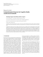
3.1. Relay-stations
The signaling interface of a relay-station is depicted in
Figure 2.Theval signals are used to propagate tokens, the
stop signals are used for congestion control. For symmetry
here stop
out is an input and stop in an output.
Intuitively the relay-station behaves as follows: when traf-
fic is clear (no stop), each token is propagated down at the

next instant from the one it was received. When a stop
out
signal is received because of downward congestion, the RS
keeps its token. But then, the previous section and the previ-
ous RS cannot be warned instantly of this congestion, and so
the current RS can perfectly well receive another token at the
same time it has to keep the former one. So there is a need
for the RS to provide a second auxiliary register slot to store
this second token. Fortunately there is no need for a third
one: in the next instant the RS can propagate back a stop
in
control information to preserve itself from receiving yet an-
other value. Meanwhile the first token can be sent as soon as
stop
out signals are withdrawn, and the RS remains with
only one value, so that in the next step it can already allow a
new one and not send its congestion control signal. Note that
in this scheme there is no undue gap between the token sent.
This informal description is made formal with the de-
scription of a synchronous circuit with two registers describ-
ing the RS in Figure 3, and its corresponding syncchart [19]
(in Mealy FSM style) in Figure 4. The syncchart contains the
following four states.
empty when no token are currently buffered in the RS; in this
state the RS simply waits for a valid input token com-
ing, and store it in its main register that then it goes to
state half. stop
out signals are ignored, and not prop-
agated upstream, as this RS can absorb traffic.
half when it holds one token; then the RS only transmits its

current, previously received token if ever does not re-
ceive an halting stop
out signal. If halting is requested,
(stop
out), then it retains its token, but must also ac-
cept a potential new one coming from upstream (as it
has not sent any back-pressure holding signal yet). In
the second case, it becomes full, with the second value
val in
stop
inval out
stop
out
MAIN AUX
(a)
data in
data
out
val
in
MUX
HALF & val
in &
stop
out
DA T A
MAIN
DA T A
AUX
FULL

01
(b)
Figure 3: Relay-station: (a) control logic, (b) data path.
Reset
empty
full
half
error
stop
out
/stop
in
val
in
val
in & stop out/
val
in/
val
in & not (stop out)
/val
out (main)
not (val
in)/
not (val
in) & not (stop out)
/val
out (main)
not (val
in)&stop out/

not (stop
out)
/stop
in, val out (aux)
Figure 4: Relay-station syncchart.
occupying its “emergency” auxiliary register. If the RS
can transmit (stop
out = false), it either goes back to
empty or retrieve a new valid signal (val
in), remain-
ing then in the same state. On the other hand it still
makes no provision to propagate back-pressure (in the
next clock cycle), as it is still unnecessary due to its own
buffering capacity.
full when it contains two tokens; then it raises in any case the
stop
in signal, propagating to the upstream section the
hold-out stop
out signal received in the previous clock
cycle. If it does not itself receive a new stop
out, then
the line downst ream was cleared enough so that it can
transmit its token; otherwise it keeps it and remains
halted.
error is a state which should never be reached (in an as-
sume/guarantee fashion). The idea is that there should
6 EURASIP Journal on Embedded Systems
be a general precondition stating that the environ-
ment will never send the val
in signal whenever the

RS emits the stop
in signal. This should be extended
to any combination of RS, and build up a “sequential
care-set” condition on system inputs. The property is
preserved as a postcondition as each RS will guarantee
correspondingly that val
out is not sent when stop out
arrives.
NB: the notation val
out(main)orval out(aux)means
emit the signal val
out taking its value in the buffer, respec-
tively, main or aux.
Correctness properties
Global correctness depends upon an assumption on the envi-
ronment (see description of error state above). We now list
a number of properties that should hold for relay-stations,
and further links made of a connected line L
n
(k)ofn succes-
sive RS elements and currently containing k values (remem-
ber that a line of n RS can store 2n values).
On a single RS:
(i) 
¬ (stop out ∧ val out) (back-pressure control takes
action immediately);
(ii)  (( stop
out ∧ X (stop out)) ⇒ X (stop in)) (a stalled
RS gets filled in two steps),
where , ♦, U,andX are the traditional Always, Even-

tually, Until,andNext (linear) temporal log ic operators.
More interesting properties can be asserted on lines of RS
elements (we assume that by renaming stop
{in, out} and
val
{in, out} signals form the I/O interface of the global line
L
n
(k)):
(i)  (¬ stop out ⇒¬X
n
(stop in)) (free slots propagate
backwards);
(ii)  ((stop
out UX
(2n−k)
(true)) ⇒ X
(2n−k)
(stop in));
(overflow);
(iii) (♦ val
in ∧  (♦ (¬ stop out)) ⇒ ♦ val out)(iftraffic
is not completely blocked from below from a point on,
then tokens get through).
The first property is true of any line of length n, the second
of any line containing initially at least k tokens, the third of
any line.
We have implemented RSs and lines of RSs in the
Esterel synchronous language, and model-checked com-
binations of these properties using EsterelStudio.

1
3.2. Shell-wrappers
The purpose of shell-wrappers is to trigger the local compu-
tation node exactly when tokens are available from each in-
put link, and there is storage available for result in output
links. It corresponds to a n otion of clock gating in circuits:
1
EsterelStudio is a trademark of Esterel Technologies.
the SW provides the logical clock that activates the IP com-
ponent represented by the CN. Of course this requires that
the component is physically able to run on such an irregu-
lar clock (a property called patie nce in LID vocabulary), but
this technological aspect is transparent to our abstract mod-
eling level. Also, it should be remembered that the CN is
supposed to produce data on all its outputs while consum-
ing on all its inputs in each computation step. This does not
imply a combinatorial behavior, since the CN itself can con-
tain internal registers of course. A more fancy framework al-
lowing computation latencies in addition to our communica-
tion latencies would have to be encoded in our formalism.
This can be done by “splitting” the node into begin
CN and
end
CN nodes, and installing internal transportation links
with desired latencies between them; if the outputs are pro-
duced with different latencies one should even split further
the node description. We will not go into further details here,
and keep the same abstraction level as in LID and WMG
theories.
The signal interface of SWs consists of val

in and
stop
in signals indexed by the number of input links to the
SW,andofval
out and stop out signals indexed by the
number of i ts output links.Thereisanoutputclock signal
in addition, to fire the local component. Thus, this last sig-
nal will b e scheduled at the rate of local firing. Note that it is
here synchronous with all the val
out signals when values
are abstracted into tokens.
The operational behavior of the SW is depicted as a syn-
chronous circuit in Figure 5(a), where each Input i module
has to be instantiated with Figure 5(b), with its signals prop-
erly renamed, finally driving the data path in Figure 5(c). The
SW is combinatorial, it takes one clock cycle to pass from RSs
before the SW, through the SW and its Pearl, and finish into
RSs in outputs of the SW.ThePearl is Patient, the state of
the Pearl is only changed when clock (periodic or sporadic)
occurs.
The SW worksasfollows:
(i) the internal Pearl’s clock and all val
out
i
valid output
signalsaregeneratedoncewehaveallval
in (signal
ALL
VAL IN in Figure 5(a)), while stop is false. The in-
ternal stop signal itself represents the disjunction of all

incoming stop
out
j
signals from outcoming channels
(signal STOP
OUT in Figure 5(a));
(ii) the buffering register of a given input channel is used
meanwhile as long as not all other input tokens are
available (Figure 5(b));
(iii) so, internal Pearl’s clock is set to false whenever a back-
ward stop
out
j
occurs as true, or a forward val in
i
is
false. In such case the registers already busy hold their
true value, wh ile others may receive a valid token “just
now;”
(iv) stop
in
i
signals are raised towards all channels whose
corresponding register was already loaded (a token w as
received before, and still not consumed), to warn them
not to propagate any value in this clock cycle. Of course
suchsignalcannotbesentincasethetokeniscurrently
received, as it would raise a causality paradox (and a
combinatorial cycle);
Julien Boucaron et al. 7

val out [1]
val
out [i]
val
out [m]
clock
= VAL OUT
ALL
VA L IN
VA L
IN [1]
STOP
OUT
stop
out [1]
stop
out [i]
stop
out [m]
VA L
IN [I]VALIN [N]
Input 1 Input i Input N
stop
in [1] stop in [i]stopin [n]
val
in [1] val in [i]valin [n]
(a)
VA L
IN [i]clock
FF-IN

FF-OUT
val
in [i]stopin [i]
DA T A
IN
FF
OUT
MUX
10
val
in & clock
DA T A
FF
data
in
(c)(b)
Figure 5: (a) Shell-wrapper circuitry, (b) input module, and (c)
data path.
(v) flip-flop registers are reset w hen the Pearl’s clock is
raised, as it consumes the input token. Following the
previous remark, the signal stop
in
i
holding back the
traffic in channel i is raised for these channels where
the tokens have arrived before the cur rent instant, even
in this case.
Correctness properties
Again we conducted a number of model-checking experi-
ments on SWs using Esterel Studio:

(i)  ((
∃ j, stop out
j
) ∨⇒¬clock)where j is an input
index;
(ii)  ((
∃ j, stop out
j
) ⇒ (∀i, ¬ val out
i
)) where j/i is an
input/output index respectively;
(iii)  ((
∀ j, ¬ stop out
j
∧¬X (stop out
j
)) ⇒ (X(clock)⇒
∃
i, X (val in
i
))) where j, i are input index (if the SW
was not suspended at some instant by output conges-
tion, and it triggers its pearl the next instant, then it has
to be because it received a new v alue token on some in-
put at this next instant).
On the other hand, most useful properties here would re-
quire syntactic sugar extensions to the logics to be easily for-
mulated (like “a token has had to arrive on each input before
or when the SW triggers its local Pearl,” but they can arrive

in any order).
As in the case of RSs, correctness also depends on the en-
vironmental assumption that
∀i, stop in
i
⇒¬val in
i
,mean-
ing that upward components must not send a value while this
part of the system is jammed.
3.3. Tool implementation
We built a prototype tool named Kpassa
2
to simulate and
analyze an LID system made of a combination of previous
components.
Simulation is eased by the following fact: given that the
ASAP synchronous semantics of LID ensures determinism,
for closed systems, each state has exactly one successor. So we
store states that were already encountered to stop the simu-
lation as soon as a state already visited is reached.
While we will come back to the main functions of the tool
in the next section, it can be used in this context of dynamic
scheduling to detect where the back-pressure control mech-
anisms are really been used, and which relay-stations actually
needed their secondary register slot to preserve from traffic
congestion.
4. SYNCHRONOUS TO LID: STATIC SCHEDULING
We now turn to the issue of providing static periodic sched-
ules for LID systems. According to the previous philosophy

governing the design of relay-stations,wewanttoprovide
solutions where tokens are not allowed to a ccumulate into
places inlargenumbers.Infactwewillattempttoequalize
the flows so that tokens arrive as much as possible simulta-
neously at their joint computation nodes.
We try to achieve our goal by adding new virtual laten-
cies on some paths that are faster than others. If such an
ideal scheme could lead to perfect equalization then the sec-
ond buffering slot mechanism of relay-stations and the back-
pressure control mechanisms could be done without alto-
gether. However, it will appear that this is not always feasible.
Nevertheless, integer latency equalization provides a close
approximation, and one can hope that the additional correc-
2
It stands for k-periodic ASAP Schedule Simulation and Analysis,pro-
nounced “Que pasa?”
8 EURASIP Journal on Embedded Systems
tion can be implemented with smaller and simpler fractional
registers.
Extra virtual latencies can often be included as computa-
tional latencies, thereby allowing the redesign of local com-
putation nodes under less stringent timing budget.
As all connected graphs, general (connected) CNSscon-
sist of directed acyclic graphs of strongly connected compo-
nents. If there is at least one cycle in the net it can be shown
that all cycles have to run at the rate of the slowest to avoid
unbounded token accumulation. This is also true of input to-
ken consumption, and output token production rates. Before
we deal with the (harder) case of strongly connected graphs
that is our goal, we spend some time on the (simpler) case of

acyclic graphs (with a single input link).
4.1. DAG case
We consider the problem of equalizing latencies in the case
of directed acyclic graphs (DAGs) with a single source com-
putation node (one can reduce DAGs to this sub-case if all
inputs are arriving at the same instant), and no initial token
is present in the DAG.
Definition 9 (DAG equalization). In this case the problem is
to equalize the DAG such that all paths arriving to a compu-
tation node are having the same latency from inputs.
We provide a sketch of the abstract algorithm and its cor-
rection proof.
Definition 10 (critical arc). An arc is defined as critical if
it belongs to a path of maximal latency Max
l
(N) from the
global source computation node to the target computation
node N of this arc.
Definition 11 (equalized computation node). A computation
node N which is having only incoming critical arcs is de-
fined to be an equalized Computation Node, that is, any path
from the source to this computation node has the same latency
Max
l
(N).
If a computation node has only one incoming arc, then
this arc will be critical and this computation node will be
equalized by definition.
The core idea of the algorithm is first to find for each
computation node N of the graph what is its maximal latency

Max
l
(N) and to mark incoming critical arcs; then the sec-
ond idea is to saturate all nonc ritical arcs of each computation
node of the DAG in order to obtain an equalized DAG.
The first part of the algorithm is done through a mod-
ified longest-path algorithm, marking incoming critical arcs
for each computation node of the DAG and putting for each
computation node N its maximal latency Max
l
(N) (as shown
in Algorithm 1).
The second part of the algorithm is done as follows (see
Algorithm 2). Since it may exist incoming arcs of a compu-
tation node N that are not critical, there exists an
 integer
number that we can add such that the noncritical arc becomes
critical. We can compute this integer number
 easily through
this formula: Max
l
(N) = Max
l
(N

)+non critical arc
l
+ ,
where N


is the source computation node passing through the
Require:GraphisaDAG
for all ARC arc of source.getOutputArcs()
do
NODE node
⇐ arc.getTargetNode();
unsigned currentLatency
⇐
arc.getLatency() + source.getLatency();
{if the latency of this path is greater}
if (node.getLatency()
≤ currentLatency)
then
arc.setCritical(true);
node.setLatency(currentLatency);
{update arcs critical field for “node”}
for all ARC node
arc o f node.getInputArcs()
do
if ( node
arc.getLatency()+
node
arc.getSourceNode().getLatency() <
currentLatency) then
node
arc.setCritical( false);
else
node
arc.setCritical(true);
end if

end for
{recursive call on “node” to update the whole
sub-graph}
recursive
longest path(node);
end if
end for
Algorithm 1: Procedure recursive longest path (NODE source).
Require:GraphisaDAG
for all NODEnodeofgraph.getNodes()do
for all ARC arc of node.getInputArcs()
do
if (arc.isCritical() == false) then
unsigned maxL
⇐ node.getLatency();
unsigned
 ⇐ maxL
- (arc.getLatency() +
arc.getSourceNode().getLatency());
arc.setLatency(arc.getLatency() +
);
arc.setCritical(true);
end if
end for
end for
Algorithm 2: Procedure final equalization (GRAPH graph).
noncritical arc and reaching the computation node N.Now,
the noncritical arc through the add of
 is critical.
We apply this for all noncritical arcs of the computation

node N, then the computation node is equalized.
Finally, we apply this for all computation nodes of the
DAG, then the DAG is equalized.
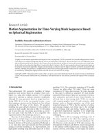
An instance of the unequalized, critical arcs annotated
and equalized DAG is shown in Figure 6.
Starting from the unequalized graph in Figure 6(a) the
following holds.
The first pass of the algorithm is determining for each
computation node its maximal latency Max
l
(in circles)
Julien Boucaron et al. 9
2
2
1
32
14
1
(a)
2
2
1
32
14
1
2
3
65
9
10

(b)
3
2
1
32
34
1
2
3
65
9
10
(c)
Figure 6: (a) Unequalized,(b)critical paths annotated (large links)
and (c) equalized DAG.
and incoming critical arcs denoted using large links as in
Figure 6(b).
The second part of the algorithm is adding “virtual” la-
tencies (the
)onnoncritical incoming arcs, since we know
the critical arcs coming through each computation node (large
links), then we just have to add the needed amount (
)inor-
der that the nonc ritical arc is now critical: the sub between
the value of the target computation node, minus the sum be-
tween the arriving critical arc and its source computation node
maximal latency. For instance, consider the computation node
holding a 9, the left branch is not critical,hencewearejust
solving 9
= 6+1+ and  = 2, thus the arc will now have

alatencyof3
= 1+ and is so critical by definition. Finally,
the whole graph will be fully-cr itical and thus equalized by
definition as in Figure 6(c).
Definition 12. A critical path is composed only of critical arcs.
Theorem 1. DAG equalization algorithm is correct.
Proof. For all computation nodes, there is at least one critical
arc incoming by definition; then if there is more than one
incoming arc, we add the result of the sub between the max-
imum latency of the path passing through the so-called crit-
ical arc and the add between the noncritical arc latency and
the maximum latency of the path arriving to the computa-
tion node where the noncritical arc starts. Now any arc on this
given computation node are all critical and thus this computa-
tion node is equalized by definition. And this is done for any
computation node, thus the graph is equalized. Since in any
case we do not modify any critical arc, we still have the same
maximum latency on critical paths.
4.2. Strongly connected case
In this case, the successive algorithmic steps involved in the
process of equalization consist in the following:
(1) evaluate the graph throughput;
(2) insert as many additional integer latencies as possible
(without changing the global throughput);
(3) compute the static schedule and its initial and periodic
phases;
(4) place fractional register s where needed;
(5) optimize the initialization phase (optional).
These steps can be il lust rated on our example in Figure 1
as follows:

(1) the left cycle in Figure 1(b) has rate 2/2
= 1, while
the (slowest) rightmost one has rate 3/5. Throughput
is thus 3/5;
(2) a single extra integer latency can be added to the link
going upward in the left cycle, bringing this cycle’s rate
to 2/3. Adding a second one would bring the rate to
2/4
= 1/2, slower than the global throughput. This
leads to the expanded form in Figure 1(c);
(3) the WMG is still not equalized. The actual schedules of
all CN can be computed (using Kpassa, as displayed in
Figure 1(d). Inspecting closely those schedules one can
notice that in all cases the schedule of a CN is the one
of its predecessors shifted right by one position, except
for the schedule of the topmost computation node.One
can deduce from the differences in scheduling exactly
when the additional buffering capacity was required,
and insert dedicated fractional registers which delay se-
lectively some tokens accordingly. This only happens
for the initial phase for tokens arriving from the right,
and periodically also for tokens arriving from the left;
(4) it could be noticed that, by advancing only the single
token at the bottom of the up going rightmost link for
one step, one reaches immediately the periodic phase,
thus saving the need for an FR element on the right
cycle used only in the initial phase. Then only one FR
has to be added past the regular latch register colored
in grey.
We describe now the equalization algorithm steps in more

detail.
Graph throughput evaluation
For this we enumerate all elementary cycles and compute
their rates. While this is worst-case exponential, it is often
not the case in the kind of applications encountered. An al-
ternative would be to use well-known “minimum mean cy-
cle problem” algorithms (see [20] for a practical evaluation
of those algorithms). But the point here is that we need all
those elementary cycles for setting up linear programming
(LP) constraints that will allow to use efficient LP solving
techniques in the next step. We are currently investigating al-
ternative implementations in Kpassa.
Integer latency insertion
This is solved by LP techniques. Linear equation systems are
built to express that all elementary cycles, w ith possible extra
variable latencies on arcs, should now be of rate R, the pre-
viously computed global throughput. The equations are also
formed while enumerating the cycles in the previous phase.
An additional requirement entered to the solver can be that
10 EURASIP Journal on Embedded Systems
the sum of added latencies be minimal (so they are inserted
in a best factored fashion).
Rather than computing a rational solution and then ex-
tracting an integer approximate value for latencies, the par-
ticular shape of the equation system lends itself well to a di-
rect greedy algorithm, stuffing incremental additional integer
latencies into the existing systems until completion. This was
confirmed by our prototype implementations.
The following example of Figure 7 shows that our inte-
ger completion does not guarantee that all elementary cycles

achieve a rate very close to the extremal. But this is here be-
cause a cycle “touches” the slowest one in several distinct lo-
cations. While the global throughput is of 3/16, g iven by the
inner cycle, no integer latency can be added to the outside
cycle to bring its rate to 1/5 from 1/4. Instead four fractional
latencies should be added (in each arc of weight 1).
Initial- and periodic-phase schedule computations
In order to compute the explicit schedules of the initial and
stationary phases we currently need to simulate the system’s
behavior. We also need to store visited state, as a termina-
tion criterion for the simulation whenever an already vis-
ited state is reached. The purpose is to build (simultaneously
or in a second phase) the schedule patterns of computation
nodes, including the quote marks (’) and (‘), so as to deter-
mine where residual fractional latency elements have to be
inserted.
In a synchronous run each state will have only one suc-
cessor, and this process stops as soon as a state already en-
countered is reached back. The main issue here consists in
the state space representation (and its complexity). Further
simplification of the state space in symbolic BDD model-
checking fashion is also possible but it is out of the scope of
this paper.
We are currently investigating (as “future work”) analytic
techniques s o as to estimate these phases without relying on
this state space constr uction.
Fractional register insertion
In an ideally equalized system, the schedules of distinct com-
putation/transportation nodes should be precisely related: the
schedule of the “next” CN should be that of the “previous”

CN shifted one slot right. If not, then extra fractional registers
need to be inserted just after the regular register already set
between “previous” and “next” nodes. This FR should delay
discriminating ly some tokens (but not all).
We will introduce a formal model of our FR in the next
subsection. The block diagram of its interfaces are displayed
in Figure 8.
We conjecture that, after integer latency equalization,
such elements are only required just before computation
nodes towherecycleswithdifferent original rates re-
converge. We prove in Section 4.4 that this is true under gen-
eral hypothesis on smooth distribution of tokens along crit-
ical cycles. In our prototypal approach we have decided to
allow them wherever the previous step indicated their need.
The intention is that the combination of a regular register

0

0

01(00001000010000

01) 00

01(000010000

0100001)
0000(00

01000010000100) 00


0

1(0000

010000100001)
1
1
1
1
4
4
4
4
Figure 7: An example of WMG where no integer latency insertion
can bring all the cycle rates the closest to the global throughput.
Previous
Next
Computation
node
Register FR
Computation
node
Figure 8: Fractional register insertion in the network.
with an additional FR register should roughly amount behav-
iorally to an RS, with the only difference that the backpres-
sure control stop
{in/out} signal mechanisms could be sim-
plified due to static scheduling information computed previ-
ously.

Optimized initialization
So far we have only considered the case where all components
did fire as soon as they could. Sometimes delaying some com-
putations or transportations in the initial phase could lead
faster to the stationary phase, or even to a distinct stationary
phase that may behave more smoothly as to its scheduling.
Consider in the example of Figure 1(c) the possibility of fir-
ing the lower-right transportation node alone (the one on the
backward up arc) in a first step. This modification allows the
graph to reach immediately the stationary phase (in its last
stage of iteration).
Initialization phases may require a lot of buffering re-
sources temporarily that will not be used anymore in the sta-
tionary phase. Providing short and buffer-efficient initializa-
tion sequences becomes a challenge. One needs to solve two
questions: first, how to generate efficiently states reachable in
an asynchronous fashion (instead of the deterministic ASAP
single successor state); second, how to discover very early that
a state may be part of a periodic regime. These issues are still
open. We are currently experimenting with Kpassa on ef-
ficient representation of asynchronous firings and resulting
state spaces.
Remark 1. When applying these successive transformation
and analysis steps, which may look quite complex, it is pre-
dictable that simple subcases often arise, due to the well-
chosen numbers provided by the designer. Exact integer
equalization is such a case. The case when fractional adjust-
ments only occur at reconvergence to critical paths are also
noticeable. We built a prototype implementation of the ap-
proach, which indicates that these specific cases are indeed

often met in practice.
Julien Boucaron et al. 11
val in & not (hold)
/val
out
val
in & hold not (val in)&hold
val
in/val out
not (catch
reg) catch reg
not (val
in)
not (val
in) & not (hold)/val out
(a)
val out
catch
reg
hold val
in
(b)
data in
catch
reg
data
out
val
in & hold
01

MUX
data
reg
(c)
Figure 9: (a) The syncchart, (b) the interface block-diagram of the FR, and (c) the datapath.
4.3. Fractional register element (FR)
We now formally describe the specific FR,bothasasyn-
chronous circuit in Figure 9(b) and as a corresponding sync-
chart (in Mealy FSM style) in Figure 9(a).
The FR interface consists of two input wires val
in and
hold, and one output wire val
out. Its internal state consists of
aregistercatch
reg. The register will be used to “kidnap” the
valid data (and its value in a real setting) for one clock cycle
whenever hold holds. We note pre(catch
reg) the (boolean)
value of the register computed at the previous clock cycle. It
indicates whether the slot is currently occupied or free.
It is possible that the same data is held several instants in
a row. But meanwhile there should be no new data arr iving,
as the FR can store only one value; otherwise this would cause
aconflict.
It is also possible that a full sequence of consecutive data
are held back one instant each in a burst fashion. But then
each data/value should leave the element in the very next in-
stant to be consumed by the subsequent computation node;
otherwise this would also cause a conflict.
Stated formally, when hold

∧ pre(catch reg) holds then ei-
ther val
in holds, in which case the new data enters and the
current one leaves (by scheduling consistency the computa-
tion node that consumes it should then be active), or val
in
does not hold, in which c ase the current data remains (and,
again by scheduling consistency, then the computation node
should be inactive). Furthermore the two extra conditions
are requested:
[hold
⇒ (val in ∨ pre(catch reg)):] if nothing can be held,
the scheduling does not attempt to;
[(val
in ∧ pre(catch reg)) ⇒ hold:] otherwise the two
pieces of data could cross the element and be output
simultaneously.
The FR behavior amounts to the two equations:
[catch
reg = hold:] the register slot is used only when the
scheduling demands;
[val
out = val out
1
∨ val out
2
:]
(i) val
out
1

= val in ⊕ pre(catch reg) ∧¬hold;
(ii) val
out
2
= val in ∧ pre(catch reg) ∧ hold.
either a new value directly falls across, or an old one is
chased by a new one being held in its place.
Our main design problem is now to generate hold signals ex-
actly when needed. Its schedule should be the difference be-
tween the schedule of its source (computation or transporta-
tion) node shifted by one instant, and the schedule of its tar-
get node; indeed, a token must be held when the target node
does not fire while the source CN did fire to produce a token
last instant, or if the token was already held at last instant.
Consider again Figure 8,wewillnamew the schedule of
the previous source CN,andw

the schedule of the next target
CN. After the regular register delay the data are produced to
the FR entry on schedule 0.w (shifted one slot/instant r ight).
The fractional register should hold the data exactly when the
kth active step at this entry is not the kth activity step at
its target CN that must consume it. In other words, the FR
resynchronize its input and output, which cannot be away
more than one activity step. This last property is true as the
schedules were computed using the LID approach with relay-
stations, which do not allow more than one extra token in ad-
dition to the regular one on each arc between computation or
transportation nodes .
Stated formally, this property becomes: hold(n)

= 1if
and only if
|0 · w
n
|
1
/= (|w

n
|
1
−|w

0
|
1
). It says that at a given
instant n we should kidnap a value if the number of occur-
rences of 1 up to instant n on the previous CN is different
than the number of occurrences of 1 on the next computation
node. More precisely, the
−|w

0
|
1
term takes care of a possible
initial activity at the target CN, not caused by the propaga-
tion of tokens from the source CN, that would have to be
removed.

Figure 10 shows a possible implementation computing
hold from signals that would explicitly provide the target and
source schedules as inputs.
Correctness properties
It can be formally proved that, under proper assumptions, a
full RS is sequentially equivalent to a system made of a reg-
ular register foll owed by a fractional one, with the respec-
tive stop
out and hold signals equated (as in Figure 11). The
exact assumption is that a stop
out/hold signal is never re-
ceived when the systems considered are already full (both
12 EURASIP Journal on Embedded Systems
reg
hold
Current N ext
Figure 10: Hold implementation.
registers occupied in each case). Providing this assumption
to a model-checker is cumbersome, as it deals with internal
states. It can thus be replaced by the fact that never in his-
tory there are more than one val
in signal received in excess
of the val
out signals sent. This can easily be encoded by a
synchronous observer.
In essence the previous property states that the two sys-
tems are equivalent safe for the emission of stop
in on a full
RS. This emission can also be shown to be simulated by in-
serting the previous HOLD component with proper inputs.

Of course, this does not mean that the implementation will
use such a dynamic HOLD pattern, but that simulating its
effect (because the static scheduling instructs us of when to
generate the signal) would make things equal to the former
RS case.
4.4. Issues of optimal FR allocation
As already mentioned in the case of an SCC we still do
not have a proof that in the stationary phase it is enough
to include such elements at the entry points of computa-
tion nodes only, so they can be installed in place of more
relay-stations also. Furthermore, it is easy to find initializa-
tionphaseswheretokensinexcesswillaccumulateatanylo-
cations, before the rate of (the) slowest cycle(s) distributes
them in a smoother, evenly distributed pattern. Still we have
several hints that partially deal with the issue. It should be re-
membered here that, even without the result, we can equalize
latencies (it just needs adding more FRs).
Definition 13 (smoothness). A schedule is called smooth if
the sequences of successive 0 (inactive) instants the differ-
ence in length between sequences of consecutive 0s cannot
differ by more than 1. The schedule (1001)

is not smooth
since they are two consecutive 0 between the first and second
occurrences of 1, while there is none between the second and
the third.
Conjecture 1. If all computation node schedules are smooth,
rates can be equalized using FR only at computation node entry
points.
Counter example 1. We originally thoug ht that Conjecture 1

should be sufficient, but the counter example of Figure 12
val out stop out
aux
main
val
in stop in
(a)
val out
stop
out
HOLD
HOLD
FR
val
in
stop
in
reg
(b)
Reset
empty
full
val
in & stop out/
val
in/
val
in & not (stop out)
/val
out (reg


FR)
reg

FR
not (val
in)&not(stop out)
/val
out (reg

FR)
not (val
in)/
not (stop
out)
/val
out (FR) + SHIFT()
not (val
in)&stop out
/+SHIFT()
SHIFT(): the data in register “reg” goes in the “FR.”
It is an internal function.
(c)
Figure 11: Equivalence of RS and FR roles.
was found. Assume a simple graph formed with two cycles
sharing one CN. The first cr itical cycle has 7 tokens and 11
latencies, the second one has 5 tokens and 7 latencies. There
exists a stationary phase w h ere the schedule of all CNsis
smooth (it is [10101010111] or any rotation of this word) but
we need two successive FRs on the noncritical cycle because

only one FR should overflow.
The reason of this failure is that the definition of smooth-
ness is not restrictive enough. In the schedule of the counter-
example Figure 12, the pattern 10 is repeated 3 times at the
beginning and we have 3 occurrences of 1 (which are not fol-
lowed by any 0) at the end. 0 and 1 are not spread regularly
Julien Boucaron et al. 13
10111101010 10101011110
01010101111
FR
C1: 5/7 C2: 7/11
Figure 12: Counter example of Conjecture 1. The FR overflow at
instant 7.
enough in the schedule. However, if the schedule of the CN
become (01011011011), we now need only one FR on the
noncritical cycle.
We propose a ne w definition.
Definition 14 (extended smoothness). A schedule w is said
to be extended smooth if any subword, with a length l,con-
tains either n bits at 1 or n + 1 bits at 1, where n is equal to
l ∗|w|
1
/|w|, |w|
1
is the number of occurrences of 1 in w
and
|w| is the length of w.
4.5. Tool implementation
Our Kpassa tool implements the various algorithmic stages
described above. Given that we could not yet prove that FRs

were only required at specific locations, the tool is ready to
insert some anywhere. Kpassa computes and displays the
system throughput, showing critical cycles and the locations
of choice for extra integer latency insertions in noncritical cy-
cles. It then computes a n explicit schedule for each computa-
tion and transportation node (in the future it could be helpful
to display only the important ones), and provides locations
for fractional registers insertion. It also provides log informa-
tion on the numbers of elements added, and whether perfect
integer equalization was achieved in the early steps.
In the future, we plan to experiment with algorithms for
finding efficient asynchronous transitory initial phases that
may reach the stationary periodic regime faster than with the
current ASAP synchronous fir ing rule.
Figure 13 displays a screen copy of Kpassa on a case
study drawn from [3]. Using the original latency specifica-
tions our tool found a static schedule using less resources
than the former implementation based on relay-stations and
dynamic back-pressure mechanisms. And now the activation
periods of components are fully predictable.
5. EXPERIMENTS ON CASE STUDIES
Tables 1 and 2 display benchmark results obtained with
Kpassa on a number of case studies. The first examples were
built from [3] for MPEG2 video encoder and from existing
and publicly available models of structural IP block diagrams
(IP MegaStore of Altera). But the latency figures were sug-
gested by our industrial partners of PACA CIM initiative. In
[18] the authors use a public-domain floorplanner to syn-
thesize approximate latency figures, based on wire lengths
induced by the placement of IPs. The last two examples are

based on graph shapes and latency distribution that are a pri-
ori adverse to the approach (without being formerly worst-
cases).
Table 1 provides features of size that are relevant to the
algorithmic complexity. Ta ble 2 reports the results obtained,
about whether perfect equalization holds, the number of
fractional registers required in the initial and p eriodic phases
(note that some FR elements may still be needed for the ini-
tial part even in perfectly equalized cases), the number of in-
teger latencies added, and time and space performances.
The current implementation of the tool is not yet opti-
mized for complexity in time and space, until now this is not
yet important. The graph state encoding is naive, and algo-
rithms are not optimal.
Kpassa isaformaltoolthatisabletocomputeeffectively
the length of initialization and periodic patterns to compute
an upper-bound of the number of resources used for the
implementation. The tool provides huge preliminary imple-
mentations for the static-scheduled LID, but it let us experi-
ment new ideas to optimize those implementations.
In addition to the results shown in Tables 1 and 2,
Kpassa also provides synthetic information on the critical-
ity of nodes: cycles can be ordered by their rates, and then
nodes by the slowest rate of a cycle it belongs to. Then the
nodes are painted from red “(Hotspot)” to blue “(Coldspot)”
accordingly. This visual information is particularly useful be-
fore equalization.
6. FURTHER TOPICS
Concerning the static scheduling, a number of important
topics are left open for further theoretical developments as

follows.
(i) Relaxing the firing rule: so far the theory developed
here only considers the case where local synchronous
components all consume and produce token on all in-
put and output channels in each computation step,
and where they all run on the same clock. In this fa-
vorable c ase functional determinacy and confluence
are guaranteed, with latencies only impacting the rela-
tive ordering of behaviors. So it can be proved that the
relaxed-synchronous version produces the same out-
put streams from the same input streams as the fully
synchronous specification (indeed the rank of a to-
ken in a stream corresponds to its time in the syn-
chronous model, thereby reconstructing the structure
of successive instants). Several papers considered ex-
tensions in the context of GALS systems, but then ig-
nored the issue of functional correspondence w ith an
initial well-clocked specification, which is our impor-
tant correctness criterion. This relaxation may help
minimize some metrics:
(a) we certainly would like to establish that FR are
needed only at computation nodes, minimizing
their number rather intuitively;
14 EURASIP Journal on Embedded Systems
Frame memory
O
∗
O
∗
+

DCT
O
∗
Quantizer
O
∗
Regulator
O
∗
Inverse quantizer
O
∗
IDCT
O
∗
O
∗
+
Input
O
∗
vPreprocessing
O
∗
Motion compensation
O
∗
Memory frame
O
∗

Motion estimation
O
∗
VLC encoder
O
∗
Buffer
O
∗
Ver tex
O
∗
(a)
Inverse quantizer
1110000001001001(0101001)
∗
IDCT
1111000000100100(1010100)
∗
(b)
Figure 13: An example simulation result (MPEG2 Encoder) w ith Kpassa. In (a), the graph; in (b), the displayed schedules for two vertices.
Table 1: Example sizes before equalization.
No. of nodes No. of cycles No. of critical cycles Max cycle latency Throughput
MPEG2 video encoder 16 7 3 21 3/7
Encoder multistandard ADPCM
12 23 23 14 1/2
H264/AVC encoder
20 12 3 27 4/9
29116a 16 bits CAST MicroCPU
11 7 3 35 3/35

Abstract stress cycles
40 2295 1 1054 4/29
Abstract stress nodes
175 3784 1 1902 4/29
(b) discovering short and efficient (minimizing
number of FR) initial phases is also an important
issue here;
(c) the distribution of integer latencies over the
arcs could attempt to minimize (on average) the
number of computation nodes that are active al-
together. In other words, transportation laten-
cies should be balanced so that computations al-
ternate in time whenever possible. The goal is
here to avoid “hot spots” that is to say flatten the
power peaks. It could be achieved by some sort of
retiming/recycling techniques and schedules ex-
ploration still using a relaxed firing rule.
(ii) Marked graphs do not allow control-flow (and con-
trol modes).Thereasonis,ingeneralcasesuchasfull
Petri Nets, it can no longer be asserted that tokens
are consumed and produced at the same rate. But ex-
plicit “branch schedules” could probably help regulate
the branching control parts by a way similar to that by
which they control the flow rate.
Finally, the goal would be to define a general GALS mod-
eling framework, where GALS components could be put in
GALS networks (to this day the framework is not compo-
sitional in the sense that local components need to be syn-
chronous). A system would consist again of computation
and interconnect communication blocks, this time each w ith

appropriate triggering clocks, and of a scheduler providing
the subclocks computation mechanism, based on their outer
main clock and several signals carrying information on con-
trol flow.
Summar y
In this a rticle we first introduced full formal models of relay
stations and Shell Wrappers, the basic components for the
theory of latency-insensitive design. Altogether they allow to
Julien Boucaron et al. 15
Table 2: Equalization performances and results (run on P4 3.4 GHz, 1 GB RAM, Linux 2.6, and JDK 1.5).
Perfect eqn. No. of FR init./periodic No. of added latencies Time Memory
MPEG2 video encoder N9/5 18< 1s ∼11 MB
Encoder multistandard ADPCM
Y 24/0 91 < 1s ∼11 MB
H264/AVC encoder
N 18/11 0 ∼ 1s ∼ 11 MB
29116a 16 bits CAST MicroCPU
Y0/0 0∼1s ∼11 MB
Abstract stress cycles
N 55/24 1577 ∼17 s ∼16 MB
Abstract stress nodes
N 59/23 2688 ∼4min ∼43 MB
build a dynamic scheduling scheme which stalls traveling val-
ues in case of congestion ahead. We established a number
of correctness properties holding between (lines of) RSs and
SWs.
Then, using former results from scheduling theory we
recognized the existence of static periodic schedules for net-
works with fixed constant latencies. We tried to use these
results to compute and optimize the allocation of buffering

resources to the system. By equalization we obtain location
where a full extra latency is always mandatory (these virtual
latencies can be later absorbed in the redesign of more re-
laxed IP components). Fractional latencies still need to be
inserted to provide per fect equalization of throughputs. By
simulation we compute the exact schedules of computation
nodes, and deduce the locations of fractional register assign-
ments to support that. We conjectured that under simple
“smoothness” assumptions on the token values distribution
along graph cycles, the FR elements could be inserted in an
optimized fashion. We also proved properties on FR imple-
mentation, and its relation to RSs.
Finally, we described a prototype implementation of the
techniques used to compute schedules and allocate integer
and fractional latencies to a system, together with prelimi-
nary benchmarks on several case studies.
ACKNOWLEDGMENTS
This work was partially supported by ST Microelectronics
and Texas Instruments grants in the context of the French
regional PACA CIM initiative.
REFERENCES
[1] L. P. Carloni, K. L. McMillan, and A. L. Sangiovanni-
Vincentelli, “Theory of latency-insensitive design,” IEEE
Transactions on Computer-Aided Design of Integrated Circuits
and Systems, vol. 20, no. 9, pp. 1059–1076, 2001.
[2] L. P. Carloni, K. L. McMillan, A. Saldanha, and A. L.
Sangiovanni-Vincentelli, “A methodology for correct-by-
construction latency insensitive design,” in Proceedings of the
IEEE/ACM International Conference on Computer-Aided De-
sign (ICCAD ’99), pp. 309–315, San Jose, Calif, USA, Novem-

ber 1999.
[3] L. P. Carloni and A. L. Sangiovanni-Vincentelli, “Performance
analysis and optimization of latency insensitive systems,” in
Proceedings of the 37th Conference on Design automation (DAC
’00), pp. 361–367, Los Angeles, Calif, USA, June 2000.
[4] T. Chelcea and S. M. Nowick, “Robust interfaces for mixed-
timing systems with application to latency-insensitive proto-
cols,” in Proceedings of the 38th conference on Design automa-
tion (DAC ’01), pp. 21–26, Las Vegas, Nev, USA, June 2001.
[5] A. Chakraborty and M. R. Greenstreet, “A minimalist source-
synchronous interface,” in Proceedings of the 15th Annual IEEE
International ASIC/SOC Conference, pp. 443–447, Rochester,
NY, USA, September 2002.
[6] F. Commoner, A. W. Holt, S. Even, and A. Pnueli, “Marked di-
rected graphs,” Journal of Computer and System Sciences, vol. 5,
no. 5, pp. 511–523, 1971.
[7] C. Ramchandani, Analysis of asynchronous concurrent systems
by timed Petri nets, Ph.D. thesis, MIT, Cambridge, Mass, USA,
September 1973.
[8] J. Carlier and P. Chr
´
etienne, Probl
`
eme d’ordonnancement:
mod
´
elisation, complexit
´
e, algorithmes, Masson, Paris, France,
1988.

[9] F. Baccelli, G. Cohen, G. J. Olsder, and J P. Quadrat, Synchro-
nization and Linearity: An Algebra for Discrete Event Syste m s,
John Wiley & Sons, New York, NY, USA, 1992.
[10] V. van Dongen, G. R. Gao, and Q. Ning, “A polynomial time
method for optimal software pipelining,” in Proceedings of the
2nd Joint International Conference on Vector and Parallel Pro-
cessing (CONPAR ’92), pp. 613–624, Springer, Lyon, France,
September 1992.
[11] F R.Boyer,E.M.Aboulhamid,Y.Savaria,andM.Boyer,“Op-
timal design of synchronous circuits using software pipelining
techniques,” in Proceedings of IEEE International Conference on
Computer Design (ICCD ’98), pp. 62–67, Austin, Tex, USA, Oc-
tober 1998.
[12] M. R. Casu and L. Macchiarulo, “A new approach to latency in-
sensitive design,” in Proceedings of the 41st Annual Conference
on Design Automation (DAC ’04), pp. 576–581, ACM Press,
San Diego, Calif, USA, June 2004.
[13] A. Cohen, M. Duranton, C. Eisenbeis, C. Pagetti, F. Plateau,
and M. Pouzet, “N-synchronous Kahn networks: a relaxed
model of synchrony for real-time systems,” in Proceedings of
the 33rd ACM SIGPLAN-SIGACT Symposium on Principles of
Programming Languages (POPL ’06), pp. 180–193, ACM Press,
Charleston, South Carolina, USA, January 2006.
[14] J. Boucaron, J V. Millo, and R. de Simone, “Another glance at
relay stations in latency-insensitive design,” Electronic Notes in
Theoretical Computer Science, vol. 146, no. 2, pp. 41–59, 2006.
[15] M. R. Casu and L. Macchiarulo, “A detailed implementation of
latency insensitive protocols,” in Proceedings of Formal Meth-
ods for Globally Asyncronous Locally Syncronous Architectures,
pp. 94–103, Pisa, Italy, September 2003.

[16] A. Benveniste, P. Caspi, S. A. Edwards, N. Halbwachs, P. Le
Guernic, and R. de Simone, “The synchronous languages 12
years later,”
Proceedings of the IEEE, vol. 91, no. 1, pp. 64–83,
2003.
16 EURASIP Journal on Embedded Systems
[17] A.V.Yakovlev,A.M.Koelmans,andL.Lavagno,“High-level
modeling and design of asynchronous interface logic,” IEEE
Design and Test of Computers, vol. 12, no. 1, pp. 32–40, 1995.
[18] M. R. Casu and L. Macchiarulo, “Floorplanning for t hrough-
put,” in Proceedings of the International Symposium on Physical
Design (ISPD ’04), pp. 62–69, ACM Press, Phoenix, Ariz, USA,
April 2004.
[19] C. Andr
´
e, “Representation and analysis of reactive behaviors: a
synchronous approach,” in Proceedings of the IMAC Multicon-
ference on Computational Engineering in Systems Applications
(CESA ’96), pp. 19–29, Lille, France, July 1996.
[20] A. Dasdan, “Experimental analysis of the fastest optimum cy-
cle ratio and mean algorithms,” ACM Transactions on Design
Automation of Electronic Systems, vol. 9, no. 4, pp. 385–418,
2004.