Báo cáo hóa học: " Research Article Efficient MPEG-2 to H.264/AVC Transcoding of Intra-Coded Video" docx

Hindawi Publishing Corporation
EURASIP Journal on Advances in Signal Processing
Volume 2007, Article ID 75310, 12 pages
doi:10.1155/2007/75310
Research Article
Efficient MPEG-2 to H.264/AVC Transcoding of
Intra-Coded Video
Jun Xin,
1
Anthony Vetro,
2
Huifang Sun,
2
and Yeping Su
3
1
Xilient Inc., 10181 Bubb Road, Cupertino, CA 95014, USA
2
Mitsubishi Electric Research Labs, 201 Broadway, Cambridge, MA 02139, USA
3
Sharp Labs of America, 5750 NW Pacific Rim Boulevard, Camas, WA 98607, USA
Received 3 October 2006; Revised 30 January 2007; Accepted 25 March 2007
Recommended by Yap-Peng Tan
This paper presents an efficient transform-domain architecture and corresponding mode decision algorithms for transcoding
intra-coded video from MPEG-2 to H.264/AVC. Low complexity is achieved in several ways. First, our architecture employs direct
conversion of the transform coefficients, which eliminates the need for the inverse discrete cosine transform (DCT) and forward
H.264/AVC transform. Then, within this transform-domain architecture, we perform macroblock-based mode decisions based
on H.264/AVC transform coefficients, which is possible using a novel method of calculating distortion in the transform domain.
The proposed method for distortion calculation could be used to make rate-distortion optimized mode decisions with lower
complexity. Compared to the pixel-domain architecture with rate-distortion optimized mode decision, simulation results show
that there is a negligible loss in quality incurred by the direct conversion of transform coefficients and the proposed transform-

domain mode decision algorithms, while complexity is significantly reduced. To further reduce the complexity, we also propose
two fast mode decision algorithms. The first algorithm ranks modes based on a simple cost function in the transform domain,
then computes the rate-distortion optimal mode from a reduced set of ranked modes. The second algorithm exploits temporal
correlations in the mode decision between temporally adjacent frames. Simulation results show that these algorithms provide
additional computational savings over the proposed transform-domain architecture while maintaining virtually the same coding
efficiency.
Copyright © 2007 Jun Xin et al. This is an open access article distributed under the Creative Commons Attribution License, which
permits unrestricted use, distribution, and reproduction in any medium, provided the original work is properly cited.
1. INTRODUCTION
The latest video compression standard, known as H.264/AVC
[1], is able to achieve significantly improved compression
efficiency over prior standards such as MPEG-2. Due to
its superior performance, it is being widely adopted for a
broad range of applications, including broadcasting, con-
sumer electronics storage, surveillance, video conference
and mobile video. As H.264/AVC becomes more widely de-
ployed, the number of devices that are capable of decod-
ing H.264/AVC bitstreams wil l g row. In fact, multiformat
standard decoder solutions, which have the capability to de-
code multiple video compression formats including MPEG-
2, H.264/AVC, and VC-1, are becoming available. This w ill
give those in the content delivery chain greater flexibility in
the format that video content is authored, edited, transmit-
ted, and stored.
However, with the success of MPEG-2 in various appli-
cation domains, there exists not only a significant amount of
legacy content, but also equipment for producing MPEG-2
content and networking infrastructure to transmit this con-
tent. To minimize the need to upgrade all of this equipment
at once and ease the transition to the new H.264/AVC coding

format, there is a strong need for efficient transcoding from
MPEG-2 to H.264/AVC. This topic has received much atten-
tion from the research community in recent years [2–4]. In
this paper, we focus on a particular subset of this larger prob-
lem, which is the transcoding of intra-coded video.
Intra-only video coding is a widely used coding method
in television studio broadcast, digital cinema, and surveil-
lance video applications. The main reason is that intra-coded
video is easier to edit than video with predictively coded
frames. Prior experiments and demonstrations have shown
that H.264/AVC intra-coding has an excellent performance,
even compared to state-of-the-art still image coding schemes
such as JPEG 2000 [5]. As an acknowledgment of such needs,
JVT is currently working on an intra-only profiles, which will
2 EURASIP Journal on Advances in Signal Processing
include tools for coding of 4 : 4 : 4 sampled video and possi-
bly lower 4 : 2 : 0 sampling formats as well [6].
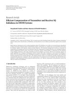
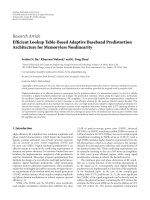
The primary aim of the transcoder in this paper is to pro-
vide more efficient network transmission and storage. A con-
ventional method of transcoding MPEG-2 intra-coded video
to H.264/AVC format is shown in Figure 1. In this architec-
ture, the transcoder first decodes an input MPEG-2 video to
reconstruct the image pixels, and then encodes the pixels in a
frame in the H.264/AVC format. We refer to this architecture
as a pixel-domain transcoder (PDT).
It is well known that transform-domain techniques may
be simpler since they eliminate the need of inverse transform
and forward transform operations. However, in the case of
MPEG-2 to H.264/AVC transcoding, the transform-domain
approach must efficiently solve the following two problems.

The first problem is a transform mismatch, which arises from
the fact that MPEG-2 uses a DCT, while H.264/AVC uses a
low-complexity integer transform, hereinafter referred to as
HT. Therefore, an efficient algorithm for DCT-to-HT coeffi-
cient conversion that is simpler than the trivial concatena-
tion of IDCT and HT is needed. A number of algorithms
that perform this conversion have been recently reported in
the literature [7–9]. Since this conversion is an important
component of the transform-domain architecture, we briefly
describe our previous work [7] and provide a comparison
to other works in this paper. The second problem with a
transform-domain architecture is in the mode decision. In
H.264/AVC, significant coding efficiency gains are achieved
through a wide variety of prediction modes. To achieve the
best coding efficiency, the rate and distortion for each cod-
ing mode are calculated, then the optimal mode is deter-
mined. In conventional architectures, the distortion is calcu-
lated based on original and reconstructed pixels with a can-
didate mode. However, in the proposed transform-domain
architecture, this distortion is calculated based on the trans-
form coefficients yielded from each candidate mode.
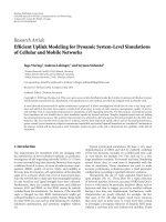
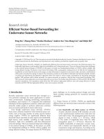
Figure 2 illustrates our proposed transform-domain
transcoder, in which the primary areas of focus are high-
lighted. In Section 2,wewilldescribewhatwerefertoasthe
S-transform, or the DCT-to-HT conversion of transform co-
efficients. Its integer implementation is also discussed. Then,
in Section 3, we present the architecture for performing a
rate-distortion optimized mode decision in the transform
domain, including a novel means of calculating distortion in
the transform domain. It is noted that the most time con-

suming operation in the transcoder is the mode decision pro-
cess, which determines the particular method for predictively
coding macroblocks. Section 4 describes a two fast mode de-
cision algorithms that achieve further speedup. Simulation
results that validate the efficiency of the various processes and
fast mode decision algorithms are discussed in Section 5.Fi-
nally, we provide a summary of our contributions and some
concluding remarks in Section 6.
2. EFFICIENT DCT-TO-HT CONVERSION
This section summarizes the key elements of our prior work
on direct conversion of transform coefficients [7]. We present
the transform matrix itself, review the fast implementation
and study the impact of integer approximations. We also dis-
cuss some of the related works in this area that have been
recently published.
2.1. Transformation matrix
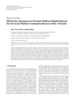
As a point of reference, Figure 3(a) shows a pixel-domain
implementation of the DCT-to-HT conversion. The input
is an 8
× 8 block (X)ofDCTcoefficients. An inverse DCT
(IDCT) is applied to X to recover an 8
× 8 pixel block (x).
The 8
× 8 pixel block is div ided evenly into four 4 × 4 blocks
(x
1
, x
2
, x
3

, x
4
). Each of the four blocks is passed to a corre-
sponding HT to generate four 4
× 4 blocks of transform co-
efficients ( Y
1
, Y
2
, Y
3
, Y
4
).Thefourblocksoftransformcoef-
ficients are combined to form a single 8
× 8 block (Y). This
is repeated for all blocks of the video.
Figure 3(b) illustrates the direct conversion of transform
coefficients, which we refer to as the S-transform.LetX de-
note an 8
× 8blockofDCTcoefficients, the corresponding
HT coefficient block Y, consisting of four 4
×4 HT blocks, is
given by
Y
= S ∗ X ∗ S
T
. (1)
As derived in [7], the kernel matrix S is
S

=
⎛
⎜
⎜
⎜
⎜
⎜
⎜
⎜
⎜
⎜
⎜
⎜
⎜
⎝
ab 0 −c 0 d 0 −e
0 fgh0
−i −jk
0
−l 0 man 0 −o
0 pj
−q 0 rgs
a
−b 0 c 0 −d 0 e
0 f
−gh0 −ij k
0 l 0
−ma−n 0 o
0 p
−j −q 0 r −gs

⎞
⎟
⎟
⎟
⎟
⎟
⎟
⎟
⎟
⎟
⎟
⎟
⎟
⎠
,(2)
where the values a
···s are (rounded off to four decimal
places)
a
= 1.4142, b = 1.2815, c = 0.45, d = 0.3007,
e
=0.2549, f =0.9236, g =2.2304, h=1.7799,
i
=0.8638, j=0.1585, k =0.4824, l=0.1056,
m
=0.7259, n=1.0864, o=0.5308, p=0.1169,
q
= 0.0922, r = 1.0379, s = 1.975.
(3)
2.2. Fast conversion

The symmetry of the kernel matrix can be utilized to design
fast implementations of the transform. As suggested by (1),
the 2D S-transform is separable. Therefore, it can be achieved
through 1D transforms. Hence, we will describe only the
computation of the 1D transform.
Let

z be an 8-point column vector, and a vector

Z the
1D transform of

z. The following steps provide a method to
Jun Xin et al. 3
Intra-
prediction
(pixel domain)
Mode
decision
Pixel
buffer
+
+
Inverse HT
Inverse Q
HT
Q
+
−
IDCT

H.264
entropy
coding
VLD/
IQ
Input MPEG-2
bitstream
VLD: variable-length decoding
(I)Q: (inverse) quantization
IDCT: inverse discrete cosine transform
HT: H.264/AVC 4
× 4transform
Figure 1: Pixel-domain intra-transcoding architecture.
Intra-
prediction
(HT domain)
Mode
decision
(HT domain)
Pixel
buffer
+
+
Inverse HT
Inverse Q
Q
+
−
DCT-to-HT conversion
(S-transform)

H.264
entropy
coding
VLD/
IQ
Input MPEG-2
bitstream
VLD: variable-length decoding
(I)Q: (inverse) quantization
IDCT: inverse discrete cosine transform
HT: H.264/AVC 4
× 4transform
Figure 2: Transform-domain intra-transcoding architecture.
determine

Z
efficiently from

z, which is also shown in
Figure 4 as a flow graph,
m1
= a × z[1],
m2
= b × z[2] −c × z[4] + d × z[6] − e × z[8],
m3
= g × z[3] − j × z[7],
m4
= f ×z[2] + h × z[4] − i × z[6] + k × z[8],
m5
= a × z[5],

m6
=−l × z[2] + m × z[4] + n × z[6] −o ×z[8],
m7
= j × z[3] + g × z[7],
m8
= p × z[2] −q × z[4] + r × z[6] + s ×z[8],
Z[1]
= m1+m2,
Z[2]
= m3+m4,
Z[3]
= m5+m6,
Z[4]
= m7+m8,
Z[5]
= m1 − m2,
Z[6]
= m4 − m3,
Z[7]
= m5 − m6,
Z[8]
= m8 − m7.
(4)
4 EURASIP Journal on Advances in Signal Processing
Y
4
Y
3
Y
2

Y
1
Y
1
Y
2
Y
3
Y
4
HT
HT
HT
HT
Inverse
DCT
x
3
x
4
x
1
x
2
x
X
(a)
Y
1
Y

2
Y
3
Y
4
Y
1
Y
2
Y
3
Y
4
S-transform
(Y
= S × X × S
T
)
X
(b)
Figure 3: Comparison between two DCT-to-HT conversion
schemes: (a) pixel domain, (b) transform domain.
This method requires 22 multiplications and 22 additions. It
follows that the 2D S-transform needs 352(
= 16 × 22) mul-
tiplications and 352 additions, for a total of 704 operations.
The pixel-domain implementation includes one IDCT
and four HT operations. Chen’s fast IDCT implementation
[10], which we refer to as the reference IDCT, needs 256(
=

16 ×16) multiplications and 416(= 16 ×26) additions. Each
HT needs 16(
= 2 × 8) shifts and 64(= 8 × 8) additions [11].
The four HT then need 64 shifts and 256 additions. It fol-
lows that the overall computational requirement of the pixel-
domain processing is 256 multiplications, 64 shifts, and 672
additions, for a total of 992 operations.
Thus, the fast S-transform saves about 30% of the oper-
ations when compared to the pixel-domain implementation.
In addition, the S-transform can be implemented in just two
stages, whereas the conventional pixel-domain processing us-
ing the reference IDCT requires six stages (four for the refer-
ence IDCT and two for the HT). In the following subsection,
an integer approximation of the S-tr ansform is described.
2.3. Integer approximation
Floating-point operations are generally more expensive to
implement than integer operations, so we also study the inte-
z[8]
z[7]
z[6]
z[5]
z[4]
z[3]
z[2]
z[1]
Z[8]
Z[4]
Z[7]
Z[3]
Z[6]

Z[2]
Z[5]
Z[1]
−1
−1
−1
−1
p
s
r
−q
−e
k
−o
g
− j
n
−id
a
m
h
−c
j
g
f
b
−l
a
Figure 4: Fast algorithm for the transform-domain DCT-to-HT
conversion.

ger approximation of the S-transform. To achieve an integer
representation, we multiply S by an integer that is a power of
two, and use the integer transform kernel matrix to perform
the transform using an integer-arithmetic. Then, the result-
ing coefficients are scaled down by proper shifting . In video
transcoding applications, the shifting operations can be ab-
sorbed in the quantization. Therefore, no additional opera-
tions are required to use integer arithmetic.
Larger integers will generally lead to better accuracy. Typ-
ically, the number is limited by the microprocessor on which
the transcoding is performed. We assume that most proces-
sors are capable of 32-bit arithmetic, so select a number that
would satisfy this constraint. However, approximations for
other processor constraints could also be determined.
The input DCT coefficients to the S-transform lie in the
range of
−2048 to 2047 and require 12 bits. The maximum
sumofabsolutevaluesinanyrowofS is 6.44, therefore
the maximum dynamic range gain for the 2D S-transform
is 6.44
2
= 41.47, which implies log
2
(41.47) = 5.4extra
bits or 17.4 bits total to represent the final S-transform re-
sults. For 32-bit arithmetic, the scaling factor must be smaller
than the square root of 2
32−17.4
, that is, 157.4. The maxi-
mum integer satisfying this condition while being a power

of two is 128. Therefore, the integer transform kernel matrix
is SI
= round{128 ×S}. Similar to S, SI has the form (2), but
with the values a through s changed to the following integers:
a
= 181, b = 164, c = 58, d = 38, e = 33,
f
= 118, g = 285, h = 228, i = 111, j = 20,
k
= 62, l = 14, m = 93, n = 139, o = 68,
p
= 15, q = 12, r = 133, s = 253.
(5)
It is noted that the fast algorithm derived in the previous
subsection for the S-transform can be applied to the above
transform since SI and S have the same symmetric property.
Also, results repor ted in [7] demonstrate that the integer S-
transform yields slight gains on the order of 0.2 dB compared
to the reference pixel-domain approach. This gain is achieved
since the integer S-transform avoids the rounding operation
Jun Xin et al. 5
Q
I
J
K
L
ABCDEFGH
a
e
i

m
b
f
j
n
c
g
k
o
d
h
l
p
0
1
34
5
6
7
8
Figure 5: (a) Neighboring samples “A-Q” are used for prediction of
samples “a-p.” (b) Prediction mode directions (except DC
Pred).
after the IDCT and for intermediate values within the HT
transform itself.
2.4. Discussion
The number of clock cycles required to execute different
types of operations are machine dependent. In the above, it
is assumed that integer addition, integer multiplication, and
shifts consume the same number of clock cycles. However,

to make the comparison more complete, let us assume that
a multiplication needs 2 cycles and an addition/shift needs 1
cycle, which is the general case for TI C64 family DSP proces-
sors. The S-transform would then need 1056(352
∗ 2 + 352)
cycles, while the conventional pixel-domain approach would
need 1248(256
∗ 2 + 64 + 672) cycles. In addition, the above
calculation has not taken into account that the reference
IDCT needs floating point operations, which typically is
more expensive than integer op erations. Therefore, the pro-
posed coefficient conversion is still more efficient.
Recently, there have been new algorithms developed for
converting D CT coefficients to HT coefficients. One algo-
rithm uses a factorized form of the 8
× 8DCTkernelma-
trix [8]. Multiplications in the process of matrix multiplica-
tions are replaced by additions and shifts. However, this pro-
cess introduces approximation errors and transcoding qual-
ity suffers. Following Shen’s method, and taking advantage
that the HT transform kernel matrix can be approximately
decomposed to the 4
× 4 DCT transform kernel, a new al-
gorithm was proposed in [ 9], where the conversion matrix
is decomposed to sparse matrices. This algorithm is shown
to b e more efficient and more accurate than [8]. Although
this approach has advantage in terms of computational com-
plexity, it still has nontrivial approximation errors compared
to our approach. More detailed comparison of the above al-
gorithms could be found in [9]. Therefore, we believe that

our proposed algorithm is preferred for high-quality appli-
cations.
3. TRANSFORM-DOMAIN MODE
DECISION ARCHITECTURE
This section describes a transform-domain mode decision
architecture, and presents a method of calculating distortion
required for cost calculations in the mode decision process.
3.1. Conventional mode decision
Let us first consider the conventional H.264 pixel-domain
mode decision (as implemented in the JM reference soft-
ware), and in particular, the rate-distortion optimized
(RDO) decision for the Intra
4 × 4modes.Figure 5(a) illus-
trates the candidate neighboring pixels “A-Q” used for pre-
diction of current 4
× 4 block pixels “a-p.” Figure 5(b) il-
lustrates the eight directional prediction modes. In addition,
DC prediction (DC
Pred) can also be used.
Consider the rate-distortion calculation in a video en-
coder with RDO
on, the conventional calculation of the La-
grange cost for one coding module (in this case for one 4
×4
luma block) is shown in Figure 6. The prediction residual is
transformed, quantized and entropy encoded to determine
the rate, R(m), for a given mode m. Then, inverse quantiza-
tion and inverse transform are performed and then compen-
sated with the prediction block to get the reconstructed sig-
nal. The distortion, denoted SSD

REC
(m), is computed as the
sum of squared distance between the original block, s,and
the reconstructed block,
s(m):
SSD
REC
(m) =


s − s(m)


2
2
,(6)
where
·
p
is the Lp-norm.TheLagrangecostiscomputed
using the rate and distortion as follows:
Cost
4×4
= SSD
REC
(m)+λ
M
∗ R(m), (7)
where λ
M

is the Lagrange multiplier, which may be calcu-
lated as a function of the quantization parameter. The opti-
mal coding mode corresponds to the mode yielding the min-
imum cost.
Besides this RDO mode selection, a low-complexity algo-
rithm, that is, with RDO
off, would only calculate the sum of
absolute distance of the Hadamard-transformed prediction
residual signal:
SATD(m)
=


T

s − s(m)



1
,(8)
where
s(m) is the prediction signal for the mode m. In this
case, the cost function would then be given by
Cost
4×4
= SATD(m)+λ
M
∗ 4 ∗


1 − δ

m = m
∗

,(9)
where m
∗
is the most probable mode for the block.
3.2. Transform-domain mode decision
The proposed transform-domain mode decision calculates
the Lagrange cost for each mode according to Figure 7,which
is based on our previous work on H.264 encoding [12]. Com-
pared to the pixel-domain approach, the transform-domain
implementation has several major differences in terms of
computation involved, which are discussed below.
First, the transform-domain approach saves one inverse
HT computation for each candidate prediction mode. This is
possible since the distortion is determined using the recon-
structed and original residual HT coefficients. The details on
this calculation are presented in the next subsection.
6 EURASIP Journal on Advances in Signal Processing
Prediction
mode
Pixel
buffers
Intra-
prediction
+
+

p
s
e
Determine
distortion
D
Inverse
HT

E
Inverse Q
Compute cost
(J
= D + λ × R)
R
Compute
rate
Q
E
HT
p
s
−
+
e
s
Figure 6: Pixel-domain RD cost calculation.
Prediction
mode
Pixel

buffer
Intra-
prediction
HT
−
+
S-transform
E
Determine
distortion
(HT-domain)
D
Inverse Q

E
Compute cost
(J
= D + λ × R)
R
Determine
rate
Q
Figure 7: Transform-domain RD cost calculation.
Second, instead of operating on the prediction residual
pixels, the HT now operates on the prediction signals. In
[12], we have shown that the HT of some intra-prediction
signals are very simple to compute. For example, there is only
one nonzero DC element in the transformed prediction sig-
nal for DC
Pred mode. Therefore, additional computational

saving are achieved.
3.3. Distortion calculation in transform domain
As described in the previous subsection and indicated in
Figure 7, the distortion is calculated in the transform do-
main, or HT domain to be precise. Since the HT is not an
orthonormal transform, it does not preserve the L2norm
(energy). However, the distortion can still be calculated with
proper coefficient weighting [12].
Let
s = p + e denote the reconstructed signal, and let
s
= p + e denote the original input signal, where e and e
are the prediction residual error signal and the reconstructed
residual signal, respectively, and p is the prediction signal.
The pixel-domain distortion, SSD
REC
(m), is given by (6).
In the following, we derive the transform-domain distortion
calculation.
First, we rewrite (6)inmatrixform:
D
= trace

(s − s) ×(s −s)
T

, (10)
where
s(m) is replaced with s for simplicity. It follows that
D

= trace

(e − e) × (e − e)
T

. (11)
Let E be the HT transformed residual signal and let

E be
the reconstructed HT transform coefficients through inverse
scaling and inverse transform. We then have the following:
e
= H
−1
× E ×

H
T

−1
, (12)
e =

H
inv
×

E ×



H
T
inv

64
, (13)
Jun Xin et al. 7
12345678
Number of modes
0.75
0.8
0.85
0.9
0.95
1
Mode prediction accuracy
Fast mode decision algorithm verification
Figure 8: Number of test modes versus accuracy.
where H and

H
inv
are the kernel matrices the forward HT
transform and inverse HT transform used in the H.264/AVC
decoding process, respectively, and are given by
H
=
⎛
⎜
⎜

⎜
⎝
11 1 1
21
−1 −2
1
−1 −11
1
−22−1
⎞
⎟
⎟
⎟
⎠
,

H
inv
=
⎛
⎜
⎜
⎜
⎜
⎜
⎜
⎜
⎜
⎜
⎜

⎝
11 1
1
2
1
1
2
−1 −1
1
−
1
2
−11
1
−11−
1
2
⎞
⎟
⎟
⎟
⎟
⎟
⎟
⎟
⎟
⎟
⎟
⎠
.

(14)
Note that in (13), the scaling after inverse HT in the decoding
process is already taken care of by the denominator 64. It is
easy to verify that

H
inv
= H
−1
× M
1
,

H
T
inv
= M
1
×

H
T

−1
,
(15)
where M
1
= diag(4, 5, 4, 5). It follows from (12), (13), and
(15) that

e
− e = H
−1
× E ×

H
T

−1
−

H
inv
×

E ×


H
T
inv

64
= H
−1
×

E −
M
1

×

E × M
1
64

×

H
T

−1
= H
−1
×

E −

E ⊗ W
1

×

H
T

−1
,
(16)
where

⊗ operator represents a scalar multiplication or entry-
wise multiplication, and W
1
is given by
W
1
=
1
64
⎛
⎜
⎜
⎜
⎝
16 20 16 20
20 25 20 25
16 20 16 20
20 25 20 25
⎞
⎟
⎟
⎟
⎠
. (17)
Initial empty
buffer
MB
0
(0,0)
MB

0
(1,0)
MB
0
(0,1)
MB
0
(1,1)
MB
0
(0,0)
MB
1
(1,0)
MB
0
(0,1)
MB
1
(1,1)
MB
0
(0,0)
MB
1
(1,0)
MB
2
(0,1)
MB

1
(1,1)
Update buffer
for all MBs
in frame
Update buffer
for MBs (1, 0)
and (1, 1)
Update buffer
for MB (0, 1)
N
N
N
N
Frame 0
R
N
R
N
Frame 1
R
R
N
R
Frame 2
Figure 9: Example of buffer updating process used for mode deci-
sion based on temporal correlation. N indicates that a new mode
decision has been made, while R indicates that the mode decision of
the previously coded macroblock is reused.
Let ΔE = E −


E ⊗ W
1
, and substituting (16) into (11)gives
D
= trace

H
−1
× ΔE ×

H
T

−1
× H
−1
× ΔE
T
×

H
T

−1

.
(18)
Denote M
2

= (H
T
)
−1
× H
−1
= diag(0.25, 0.1, 0.25, 0.1), we
also have (H
T
)
−1
= M
2
× H, which then gives
D
= trace

H
−1
× ΔE × M
2
× ΔE
T
× M
2
× H

=
trace


ΔE × M
2
× ΔE
T
× M
2

=


ΔE ⊗ W
2


2
2
,
(19)
where W
2
is given by
W
2
=
⎛
⎜
⎜
⎜
⎜
⎜

⎜
⎜
⎜
⎜
⎜
⎜
⎜
⎝
1
4
1
√
40
1
4
1
√
40
1
√
40
1
10
1
√
40
1
10
1
4

1
√
40
1
4
1
√
40
1
√
40
1
10
1
√
40
1
10
⎞
⎟
⎟
⎟
⎟
⎟
⎟
⎟
⎟
⎟
⎟
⎟

⎟
⎠
. (20)
Expanding ΔE gives the final forms of the transform-domain
distortion:
D
HT
(m) =



E −

E(m) ⊗ W
1

⊗
W
2


2
2
. (21)
Thus far, we have shown that with weighting matrices W
1
and W
2
to compensate for the different norms of HT, inverse
HT and H.264/AVC quantization design, we can calculate the

SSD distortion in the HT domain using (21).
In what follows, we analyze the computational complex-
ity of the proposed distortion calculation. All following dis-
cussions are based on a 4
× 4 block basis. In (21), to avoid
floating point operation in computing (

E(m) ⊗W
1
), we take
the 1/64 constant out of the L2-norm operator to yield
D
HT
(m) =
1
64
2



64 ∗ E −

E(m) ⊗

WI
1

⊗
W
2



2
2
, (22)
8 EURASIP Journal on Advances in Signal Processing
where WI
1
= 64 ∗ W
1
is now an integer matrix. Let Y =
64 ∗ E −

E(m) ⊗ WI
1
, and substituting W
2
into ( 22)gives
D
HT
=
1
64
2

Y(1,1)
2
+ Y(1,3)
2
+ Y(3,1)

2
+ Y(3,3)
2
16
+
Y(2,2)
2
+ Y(2,4)
2
+ Y(4,2)
2
+ Y(4,4)
2
100
+
Y(1,2)
2
+ Y(1,4)
2
+ Y(2,1)
2
+ Y(4,1)
2
40
+
Y(2,3)
2
+ Y(3,2)
2
+ Y(3,4)

2
+ Y(4,3)
2
40

.
(23)
Compared to the pixel-domain distor tion calculation
in (6), the additional computations include computing Y,
specifically 64
∗E and

E(m)⊗WI
1
, 1 shift (/16), and 2 integer
divisions. In computing Y,64
∗E needs 16 shifts, but it only
needs to be precomputed once for all modes to be evaluated.
Computing

E(m) ⊗ WI
1
requires 16 integer multiplications.
Overall, the additional operations at most include 16 multi-
plications, 2 divisions, and 17 shifts, for a total of 35 opera-
tions.
On the other hand, to calculate the distortion using the
pixel-domain method according to (6), inverse transform
and reconstruction are necessary to reconstruct
s. The in-

verse transform needs 64 additions and 16 shifts [13] and the
reconstruction needs 16 additions (subtractions). Therefore,
the additional operations compared to (6) are 80 additions
and 16 shifts, for a total of 96 operations.
From the above analysis, it is apparent that the proposed
transform-domain distortion calculation is more efficient
than the traditional pixel-domain approach. It should also
be noted that the proposed mode decision architecture has
additional advantages as explained in Section 3.2.
4. FAST MODE DECISION ALGORITHMS
4.1. Ranking-based mode decision
For optimal coding performance, the H.264 coder utilizes
Lagrange coder control to optimize mode decisions in the
rate-distortion sense. When lower complexity is desired, the
SATD cost in (9) is used, which requires much simpler com-
putation. Using the SATD cost reduces coding performance
since the cost function is only an approximation of the ac-
tual RD cost given by (7). In this subsection, we propose a
fast intra mode decision algorithm that is based on the fol-
lowing observation: although choosing the mode with the
smallest SATD value often misses the best mode in the RD
sense, the best mode usually contains smaller SATD cost. In
other words, the mode rankings according to the two cost
functions are highly correlated.
The basic idea is to rank all candidate modes using the
less complex SATD cost, and then evaluate Lagrange RD costs
only for the few best modes decided by the ranking. Based on
the input HT coefficients of prediction residual signal, the
algorithm is described in the following.
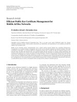
PDT TDT TDT-C1 TDT-C2 TDT-C3 TDT-R RDOoff

0
10
20
30
40
50
60
70
80
90
100
(%)
Akiyo
Mobile
Stefan
Figure 10: Complexity of proposed transcoders (%) relative to
PDT. The threshold values used for Akiyo for TDT-C1, TDT-C2,
TDT-C3 are 512, 1024 and 2048 respectively, and for mobile and
Stefan, they are 12228, 16834, 24576, and 4096, 12228, 16384, re-
spectively.
First, we compute the HT domain c
1
for all candidate
modes based on normalized HT-domain residual coeffi-
cients:
c
1
(m) =



(S −

S(m)

⊗
W
2


1
+ λ
M
∗ 4 ∗

1 − δ

m = m
∗

.
(24)
Then, we sort the modes according to c
1
in ascending or-
der, putting the first k smallest modes in the test set T.Next,
we add DC
Pred into T if it is not in T already. For the modes
in T,compute
c
2

(m) =



E −

E ⊗ W
1

⊗
W
2


2
2
+ λ
M
∗ R(m). (25)
We finally select the best mode according to c
2
(m).
Note that in calculating (9), instead of using Hadamard
transform, the distortion SATD is defined as the SAD
of HT coefficients since they are already available in the
transform-domain transcoder. The parameter k controls the
complexity-quality tradeoff. To verify the correlations be-
tween rankings using c
1
and c

2
, a simple experiment is per-
formed. We collect the two costs for all luma 4
× 4 blocks
in the first frame of all CIF test sequences (see next section)
coded with QP
= 28, and then count the percentage of times
when the best mode according to c
2
is in the test set T. This is
called the mode prediction accuracy. The results are plotted
in Figure 8 as k versus accuracy. The strong correlation be-
tween the two costs is evident in the high accuracies shown.
In this work, k is set to be 3.
4.2. Exploiting temporal correlation
It is well known that strong correlations exist between adja-
cent pictures, and it is reasonable to assume that the optimal
mode decision results of collocated macroblocks in two adja-
cent pictures are also strongly correlated. In our earlier work
Jun Xin et al. 9
Table 1: RD performance comparisons with QP = 27. Bitrate:
kbps, PSNR: dB.
Akiyo Foreman Container Stefan
PDT
Bitrate 1253.2 1695.48 2213.6 3807.4
PSNR 40.40 37.30 36.24 34.63
TDT
Bitrate 1577.4 2229.1 2905.1 4812.1
PSNR 40.38 37.28 36.21 34.63
TDT-R

Bitrate 1579.1 2233.3 2907.9 4809.2
PSNR 40.35 37.27 36.18 34.57
Table 2: RD performance comparisons with QP = 30. Bitrate:
kbps, PSNR: dB.
Akiyo Foreman Container Stefan
PDT
Bitrate 1253.2 1659.48 2213.6 3807.4
PSNR 38.63 35.84 34.77 33.26
TDT
Bitrate 1258.04 1654.16 2207.19 3795.8
PSNR 38.59 35.83 34.75 33.25
TDT-R
Bitrate 1257.72 1656.48 2208.46 3789.8
PSNR 38.59 35.82 34.72 33.19
[14], we proposed a fast mode decision algorithm for intra-
only encoding that exploits the temporal correlation in mode
decisions of a djacent pictures. In this subsection, we present
the corresponding algorithm that could be within the context
of the transform-domain transcoding architecture.
One key step to exploit temporal correlations of mac-
roblock modes is to first measure the difference between
the current macroblock and its collocated macroblock in the
previously coded picture. If they are close enough, the cur-
rent macroblock will reuse the mode decision of its collo-
cated macroblock and the entire mode decision process is
skipped. In our earlier work, we measured the degree of
correlation between two macroblocks in the pixel domain
according to a difference measure that accounted not only
for the differences between collocated macroblocks, but also
the pixels used for intra-prediction of that macroblock. This

pixel-domain distance measure may not be applied in the
transform-domain architecture since we do not have access
to pixel values. We propose to use a distance measure cal-
culated in the transform domain as follows to measure the
temporal correlation:
D
=


S − S
col


1
, (26)
where S is the HT coefficients of current macroblock, and
S
col
is the HT coefficients of the collocated macroblock. Note
that we did not try to include the pixels outside of current
macroblock that may be used for intra-prediction. These pix-
els are difficult to include in the transform-domain distance
measure. However, our simulations results show that the ex-
clusion of these pixels did not cause noticeable performance
penalty.
for all MBs in picture do
Compute D between the current MB and associated MB
stored in the buffer based on (26)
if D>THthen
Perform mode decision for the current MB

U pdate buffer with current MB data
else
Reuse mode decision of the collocated MB in the
previous picture
end if
end for
Algorithm 1: Mode decision based on temporal correlation.
The next important element of the proposed algorithm
is to prevent accumulation of the distortion resulting from
mode reuse. This requires an additional buffer that is up-
dated with coefficients of the current input macroblock only
when there is a new mode decision. This strategy allows for
differences to be measured based on the original macroblock
that was used to determine a particular encoding mode. If the
differences were taken with respect to the immediately previ-
ous frame, then it would become possible that small differ-
ences, that is, less than the threshold, over time would not
be detected. In that case, an encoding mode would continue
to be reused even though the macroblock characteristics over
time have changed significantly.
Figure 9 shows the buffer updating process for several
frames containing four macroblocks each. For Frame 0,
the mode decisions for all four macroblocks are newly de-
termined and denoted with an N. The macroblock data
from frame 0 {MB
0
(0, 0), MB
0
(0, 1), MB
0

(1, 0), MB
0
(1, 1)}
are then stored in the frame buffer. For Frame 1, the mode
decision has determined that the encoding modes for mac-
roblocks (0,0) and (0,1) will be reused, which are denoted
with an R, while the encoding modes for macroblocks (1,0)
and (1,1) are newly determined. As a result, the buffer is up-
dated with the corresponding macroblock data from frame 1
{MB
1
(1, 0), MB
1
(1, 1)};dataforothermacroblocksremain
unchanged. For Frame 2, only macroblock (0,1) has been
newly determined, therefore the only update to the frame
buffer is {MB
2
(0, 1)}.
It is evident from the above example that the buffer
is composed of a mix of macroblock data from different
frames. The source of the data for each macroblock repre-
sents the frame at which the encoding mode decision was
been determined. The data in the buffer is used as a refer-
ence to determine whether the current input macroblock is
sufficiently correlated and whether the macroblock encoding
mode could be reused.
The complete algorithm is given in Algorithm 1.
The threshold TH can be used to control the quality-
complexity tr adeoff.AlargerTH leads to lower quality, but

faster mode decision and hence lower computational com-
plexity.
10 EURASIP Journal on Advances in Signal Processing
0.80.911.11.21.31.41.51.61.71.81.922.12.2
Bitrate (Mbps)
34
35
36
37
38
39
40
41
42
PSNR-Y (dB)
PDT
TDT
TDT-C(512)
TDT-C(1024)
TDT-C(2048)
PDT-RDOoff
(a)
3456789
Bitrate (Mbps)
26
27
28
29
30
31

PSNR-Y (dB)
PDT
TDT
TDT-C(12228)
TDT-C(16834)
TDT-C(24576)
PDT-RDOoff
(b)
22.533.544.55 5.566.5
Bitrate (Mbps)
29
30
31
32
33
34
35
36
PSNR-Y (dB)
PDT
TDT
TDT-C(4096)
TDT-C(12228)
TDT-C(16834)
PDT-RDOoff
(c)
Figure 11: RD performance evaluation of TDT-C transcoder with
different thresholds: (a) Akiyo; (b) Mobile; (c) Stefan.
Table 3: RD performance comparisons with QP
= 33. Bitrate:

kbps, PSNR: dB.
Akiyo Foreman Container Stefan
PDT
Bitrate 993.2 1249.0 1673.9 2904.8
PSNR 36.72 34.29 33.19 31.59
TDT
Bitrate 993.2 1246.6 1671.3 2899.5
PSNR 36.74 34.27 33.18 31.58
TDT-R
Bitrate 993.9 1248.0 1673.4 2896.5
PSNR 36.73 34.27 33.16 31.52
5. SIMULATION RESULTS
In this section, we report results to demonstrate the ef-
fectiveness of the proposed architectures and algorithms.
We compare the coding efficiency and complexity of the
pixel-domain transcoder (PDT) to the transform-domain
transcoder (TDT) with RDO turned on. The PDT, as shown
in Figure 1, uses conventional coefficient conversion method
and conventional mode decision algorithm. Chen’s fast
IDCT implementation [10] is used in MPEG-2 decoding.
In TDT, as shown in Figure 2, the proposed transcoding
architecture, integer DCT-to-HT conversion (Section 2.3),
and transform-domain mode decision (Section 3 ) are imple-
mented. We also evaluate the performance of the proposed
fast mode decision algorithms (Section 4) within the context
of the TDT architecture, namely the fast mode decision based
on ranking (TDT-R) and the algorithm based on temporal
correlation (TDT-C). Comparisons are made to the PDT ar-
chitecture w ith RDO on and off.
The experiments are conducted using 100 frames of stan-

dard test sequences at CIF resolution. The sequences are all
intra-encoded at a frame rate of 30 Hz and bit-rate of 6 Mbps
using the public domain MPEG-2 software [15]. The result-
ing bitstreams are then transcoded using the various archi-
tectures. The transcoders are implemented based on MSSG
MPEG-2 software codec and H.264 JM7.6 reference code
[16].
Tables 1–3 summarize the RD performance of the ref-
erence transcoder, that is, PDT, and proposed transcoders,
TDT and TDT-R, while Figure 10 shows the complexity re-
sults for two sequences and QP 30. Results are similar for
other sequences and QP values. It is noted that the complex-
ity is measured by the CPU time consumed by transcoders.
All simulations are performed on a PC running Windows XP
with an Intel Pentium-4 CPU 2.4 GHz. The software is com-
piled with the Intel C++ Compiler v7.0. Several key observa-
tions regarding the results are discussed below.
The first notable point is that the TDT architecture
achieves virtually the same RD performance as PDT. Also, the
computational savings of TDT over PDT are typically around
20%. These savings come partly from the reduced complexity
achieved by the S-transform compared to pixel-based con-
version and partly from the reduced complexity in the mode
Jun Xin et al. 11
decision process. Recall that both architectures employ RDO,
but the mode decision in the transform-domain architec-
ture performs the distortion calculation in the transform-
domain, thereby eliminating certain operations.
If we further analyze the performance of TDT-R, we ob-
serve that this algorithm saves approximately 50% of the

computation compared to the PDT architecture. Compared
to the TDT architecture with full RDO, up to 30% savings
are achieved. Furthermore, these computational savings are
achieved with negligible degradation in PSNR. The results
show less than 0.1 dB loss for all test cases.
The simulation results using various threshold values for
transcoder TDT-C are shown in Figure 11. In this figure, each
RD curve is generated using 5 different QP values: 24, 27, 30,
33, and 36. As references, we plot PDT with RDO on and
off, as well as TDT. The complexity comparison is shown
in Figure 10. It can be seen that different threshold values
provide different tradeoffsofRDperformanceandcomputa-
tional complexities. Relative to TDT, up to 40% computation
can be saved with less than 0.2 dB loss in quality. These results
show that turning off RDO provides the lowest complex-
ity, but also results in lower quality. For the three sequences
shown in the figure, the quality degradation is in the range of
0.2–0.4 dB. The benefits of the TDT-C scheme is that it offers
flexible tradeoffs between coding efficiency and complexity.
Both TDT-R and TDT-C provide significant saving in
complexity relative to exhaustive RDO algorithm. It appears
though that TDT-R is a more effective approach since it in-
curs almost no loss in RD performance and achieves compa-
rable complexity reduction to TDT-C. Perhaps a combina-
tion of the two approaches would yield further complexity
reduction and better tradeoff.
6. CONCLUSIONS
We propose d an efficient transform-domain MPEG-2 to
H.264 intra-video transcoder. The transform-domain archi-
tecture is equivalent to the conventional pixel-domain im-

plementation in terms of functionality, but it has signifi-
cantly lower complexity with no loss in coding efficiency.
We achieved complexity reduction with a transform-domain
architecture that utilizes a direct DCT-to-HT coefficient
conversion and a transform-domain mode decision. The
transform-mode decision is enabled by calculating distortion
based on transform coefficients. We also presented two fast
mode decision algorithms that are able to operate within the
context of the transform-domain architecture. Both of these
algorithms demonstrated that further reductions in com-
plexity with neg ligible loss in quality could be achieved.
REFERENCES
[1] “ITU-T Rec. H.264—ISO/IEC 14496-10: Advanced Video
Coding,” 2003.
[2] Z. Zhou, S. Sun, S. Lei, and M T. Sun, “Motion information
and coding mode reuse for MPEG-2 to H.264 transcoding,” in
Proceedings of IEEE International Symposium on Circuits and
Systems (ISCAS ’05), vol. 2, pp. 1230–1233, Kobe, Japan, May
2005.
[3] X. Lu, A. M. Tourapis, P. Yin, and J. Boyce, “Fast mode deci-
sion and motion estimation for H.264 with a focus on MPEG-
2/H.264 transcoding,” in Proceedings of IEEE International
Symposium on Circuits and Systems (ISCAS ’05), vol. 2, pp.
1246–1249, Kobe, Japan, May 2005.
[4] T. Qian, J. Sun, D. Li, X. Yang, and J. Wang, “Transform do-
main transcoding from MPEG-2 to H.264 with interpolation
drift-error compensation,” IEEE Transactions on Circuits and
Systems for Video Technology, vol. 16, no. 4, pp. 523–534, 2006.
[5] K. B. Bruce, L. Cardelli, and B. C. Pierce, “Comparing object
encodings,” in Proceedings of 3rd International Symposium on

Theoretical Aspects of Computer Software (TACS ’97),M.Abadi
and T. Ito, Eds., vol. 1281 of Lecture Notes in Computer Science,
pp. 415–438, Springer, Sendai, Japan, September 1997.
[6] H. Yu, “Joint 4:4:4 Video Model (JFVM) 2,” JVT-R205, 2006.
[7] J. Xin, A. Vetro, and H. Sun, “Converting DCT coefficients
to H.264/AVC transform coefficients,” in Proceedings of IEEE
Pacific-Rim Conference on Multimedia (PCM ’04), vol. 2, pp.
939–946, Tokyo, Japan, November 2004.
[8] B. Shen, “From 8-tap DCT to 4-tap integer-transform for
MPEG to H.264/AVC transcoding,” in Proceedings of the In-
ternational Conference on Image Processing (ICIP ’04), vol. 1,
pp. 115–118, Singapore, October 2004.
[9] C. Y. Park and N. I. Cho, “A fast algorithm for the conversion of
DCT coefficients to H.264 transform coefficients,” in Proceed-
ings of the International Conference on Image Processing (ICIP
’05), vol. 3, pp. 664–667, Genova, Italy, September 2005.
[10] W H Chen, C. Smith, and S. Fralick, “A fast computation al-
gorithm for the discrete cosine transform,” IEEE Transactions
on Communications, vol. 25, no. 9, pp. 1004–1009, 1977.
[11] H. S. Malvar, A. Hallapuro, M. Karczewicz, and L. Kerofsky,
“Low-complexity transform and quantization in H.264/AVC,”
IEEE Transactions on Circuits and Systems for Video Technology,
vol. 13, no. 7, pp. 598–603, 2003.
[12] J. Xin, A. Vetro, and H. Sun, “Efficient macroblock coding-
mode decision for H.264/AVC video coding,” in Proceedings of
the 24th Picture Coding Symposium (PCS ’04), pp. 53–58, San
Francisco, Calif, USA, December 2004.
[13] A. Hallapuro, M. Karczewicz, and H. Malvar, “Low complexity
transform and quantization—part II: extensions,” JVT-B039,
2002.

[14] J. Xin and A. Vetro, “Fast mode decision for intra-only
H.264/AVC coding,” in Proceedings of the 25th Picture Coding
Symposium (PCS ’06), Beijing, China, April 2006.
[15] “MPEG-2 encoder/decoder v1.2,” 1996, by MPEG Software
Simulation Group, />[16] “H.264/AVC reference software JM7.6,” 2003, http://iphome
.hhi.de/suehring/tml/download/.
Jun Xin received the B.E. degree from
Southeast University, Nanjing, China, in
1993, the M.E. degree from Institute of
Automation, Chinese Academy of Sciences,
Beijing, China, in 1996, and the Ph.D. de-
gree from University of Washington, Seat-
tle, Wash, USA in 2002, al l in electrical en-
gineering. Since August 2003, he has been
with Mitsubishi Electric Research Laborato-
ries (MERL), Cambridge, Mass, USA. From
1996 to 1998, he was a Software Engineer at Motorola-ICT Joint
R&D Lab, Beijing, China. His research interests include digital
video compression and communication. He has been an IEEE
Member since 2003.
12 EURASIP Journal on Advances in Signal Processing
Anthony Vetro received the B.S., M.S., and
Ph.D. degrees in electrical engineering from
Polytechnic University, Brooklyn, NY. He
joined Mitsubishi Electric Research Labs,
Cambridge, Mass, USA, in 1996, where he
is currently a Senior Team Leader and re-
sponsible for research related to the encod-
ing, transport, and consumption of multi-
media content. He has published more than

100 papers and has been an active member
of the MPEG and JVT Standardization Committee for several years.
He is currently serving as an Editor for multiview video coding
amendment of H.264/AVC. Dr. Vetro serves on the program com-
mittee for various conferences and has held several editorial posi-
tions. He is currently an Associate Editor for IEEE Signal Processing
Magazine and Chair-Elect of the Technical Committee on Multi-
media Signal Processing of the IEEE Signal Processing Society, as
well as the Technical Committees on Visual Signal Processing and
Communications and Multimedia Systems and Applications of the
IEEE Circuits and Systems Society. He recently served as a Confer-
ence Chair for ICCE 2006 and a Tutorials Chair for ICME 2006,
and has been a Member of the Publications Committee of the IEEE
Transactions on Consumer Electronics since 2002. Dr. Vetro has
also received several awards for his work on transcoding, including
the 2003 IEEE Circuits and Systems CSVT Transactions Best Paper
Award and the 2002 Chester Sall Award. He is a Senior Member of
the IEEE.
Huifang Sun graduated from Harbin En-
gineering Institute, Harbin, China, and re-
ceived the Ph.D. degree from University of
Ottawa, Canada. He joined Electrical Engi-
neering Department of Fairleigh Dickinson
University as an Assistant Professor in 1986
and was promoted to an Associate Profes-
sor before moving to Sarnoff Corporation
in 1990. He joined Sarnoff Lab as a mem-
ber of technical staff and was promoted to a
Technology Leader of Digital Video Communication later. In 1995,
he joined Mitsubishi Electric Research Laboratories (MERL) as Se-

nior Principal Technical Staff and was promoted as Vice President
and Fellow of MERL and Deputy Director of Technology Lab in
2003. His research interests include digital video/image compres-
sion and digital communication. He has coauthored two books and
more than 130 journal/conference papers. He holds 43 US patents
and has more pending. He received Technical Achievement Award
for optimization and specification of the Grand Alliance HDTV
video compression algorithm in 1994 at Sarnoff Lab. He received
the Best Paper Award of 1992 IEEE, Transaction on Consumer Elec-
tronics, the Best Paper Award of 1996 ICCE, and the Best Paper
Award of 2003 IEEE Transaction on CSVT. He is now an Asso-
ciate Editor for IEEE Transaction on Circuits and Systems for Video
Technology and was the Chair of Visual Processing Technical Com-
mittee of IEEE Circuits and System Society. He is an IEEE Fellow.
Yeping Su was born in Rugao, Jiangsu,
China. He received his Ph.D. degree (2005)
in electrical engineering at the University
of Washington, Seattle. He interned for
EnGenius Technologies at Bellevue, Wash,
USA (2001), Microsoft Research at Red-
mond, Wash, USA (2003), and Mitsubishi
Electric Research Labs at Cambridge, Mass,
USA (2004). He was a member of technical
staff at Thomson Corporate Research Lab
at Princeton, NJ, from 2005 to 2006. He is currently a member of
technical staff at Sharp Labs of America at Camas, Wash.