Báo cáo hóa học: " Research Article Self-Timed Scheduling Analysis for Real-Time Applications" doc

Hindawi Publishing Corporation
EURASIP Journal on Advances in Signal Processing
Volume 2007, Article ID 83710, 14 pages
doi:10.1155/2007/83710

Research Article
Self-Timed Scheduling Analysis for Real-Time Applications
Orlando M. Moreira and Marco J. G. Bekooij
NXP Semiconductors Research, 5656 AE Eindhoven, The Netherlands
Received 1 September 2006; Accepted 2 April 2007
Recommended by Roger Woods
This paper deals with the scheduling analysis of hard real-time streaming applications. These applications are mapped onto a
heterogeneous multiprocessor system-on-chip (MPSoC), where we must jointly meet the timing requirements of several jobs.
Each job is independently activated and processes streams at its own rate. The dynamic starting and stopping of jobs necessitates
the usage of self-timed schedules (STSs). By modeling job implementations using multirate data flow (MRDF) graph semantics,
real-time analysis can be performed. Traditionally, temporal analysis of STSs for MRDF graphs only aims at evaluating the average
throughput. It does not cope well with latency, and it does not take into account the temporal behavior during the initial transient
phase. In this paper, we establish an important property of STSs: the initiation times of actors in an STS are bounded by the
initiation times of the same actors in any static periodic schedule of the same job; based on this property, we show how to guarantee
strictly periodic behavior of a task within a self-timed implementation; then, we provide useful bounds on maximum latency for
jobs with periodic, sporadic, and bursty sources, as well as a technique to check latency requirements. We present two case studies
that exemplify the application of these techniques: a simplified channel equalizer and a wireless LAN receiver.
Copyright © 2007 O. M. Moreira and M. J. G. Bekooij. This is an open access article distributed under the Creative Commons
Attribution License, which permits unrestricted use, distribution, and reproduction in any medium, provided the original work is
properly cited.

1.

INTRODUCTION

1.1. Application domain

In order to deliver high-quality output, streaming media applications have tight real-time (RT) requirements. These typically come in several different flavors [1], according to the
type of requirements. For instances, in hard real time the
deadlines of jobs cannot be missed, while in soft real time the
deadlines can be missed, but the rate of misses must be kept
below a specified maximum. Because human perception is
more tolerant of frame loss in a video signal than sample loss
in an audio signal, video applications are often implemented
as soft real time, while most radio and audio applications are
treated as hard real time.
Contrarily to real-time control applications where most
temporal requirements are in terms of latency, the temporal requirements of real-time streaming applications are
mostly throughput oriented, although latency requirements
may still be present.
Embedded platforms for streaming are expected to handle several streams at the same time, each with its own rate.
Typically, functionality can be divided in minimal groups of
interconnected tasks that can be started and stopped inde-

pendently by an external source such as the user. We refer to
such groups of tasks as jobs. The connections among tasks
within a job are static. Jobs can be connected dynamically
to each other by feeding the output of one as an input to
another. This is done, for instance, when equalization is applied to the output of an audio decoder. The number of use
cases (a use case is a combination of simultaneously executing job instances that the device must support) is potentially
very high.
This application domain includes car infotainment [2],
where the user can request at any moment radio baseband
processing for either AM or FM, or digital decoding or encoding for one of many audio formats. Several streams can
be present at a time, both because independent sound output
must be provided to front and backseat, and different streams
may be mixed (such as when listening to music while receiving a phone call). Moreover, further sound processing may

be provided, such as equalization or echo cancellation for a
hands-free phone kit.
1.2.

Hardware issues

For embedded hardware platforms, multiprocessor systemson-chip (MPSoCs) provide a good balance between cost,


1.3. Our approach
1.3.1. Hardware requirements
Our model-based approach can only be exploited to the
fullest when some restrictions are imposed to the hardware.
We think that these restrictions become necessary to make
the design of complex MPSoCs manageable.
Under this perspective, the most desirable feature of an
MPSoC is resource virtualization: a job may see and use only
the part of the system resources that is reserved for it. This
implies that resource reservation is done a priori. Virtualization makes a system composable. Because of this, we prescribe the usage of networks-on-chip (NoCs) such as the
Ỉthereal [3, 4], which allow the definition of connections
with guaranteed throughput and latency, therefore isolating
each communication channel from the rest of the system. To
enable virtualization, all arbitration mechanisms in the SoC
should provide guarantees of a rather tight upper bound to
the waiting time for resource provision. We refer to such arbitration mechanisms as predictable.
In this paper, we restrict ourselves to SoCs where every
processor has its own local dedicated memory. Shared memory can be handled by our analysis techniques, but its access must be arbitrated in a predictable fashion. We assume
that caches are not used. This is fine for hard-real-time applications, since little advantage can be taken from the probabilistic performance improvement offered by caching. Again,
the next-generation Car Infotainment system we use as case

NI

X

NI

NI

P

EPICS

Y

Y
X

CA

X

P

EPICS

Y

CA

X

P

EPICS

EPICS

P
Y

CA

power efficiency, and flexibility. These systems are typically
heterogeneous, as the usage of application-specific coprocessors can greatly improve performance at low area cost. Also,
it is likely that the need for scalability and ease of design will
drive these systems towards the usage of uniform networkson-chip (NoCs) [3] for interprocessor communication.
In order to allow maximum flexibility at the lowest cost,
jobs share computation, storage, and communication resources. This poses a particularly difficult problem for the
programming of real-time applications. Resource sharing
leads to uncertainty of resource provision which can make
the system noncomposable, that is, the temporal behavior of
each job becomes dependent on other jobs and cannot be
verified in isolation. As the current software verification processes rely strongly on extensive simulation, a large number
of tests would have to be carried out in order to verify all
possible use cases. Even if this were feasible, few guarantees
could be given, since the simulation results only apply for the
particular data streams that were used for testing. This is unacceptable for hard-real-time systems.
We are convinced that the solution to these mounting
problems requires a shift to a more analytical, model-based
approach. Although we do believe that extensive testing and

simulation may still be necessary in many cases, we try to see
how far we can go with a strictly model-based approach. This
is, however, far more than a theoretical exercise. In fact, the
techniques we developed are being applied to the design of an
MPSoC for a next-generation Car Infotainment system [2].

EURASIP Journal on Advances in Signal Processing

CA

2

NI

Ỉthereal network
NI

NI

NI

NI

CA
crd

fir

crd

Src

IFAD
IIS

AD

ARM-based
subsystem

DA

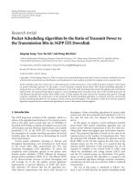
Figure 1: Next-generation car infotainment system architecture.

study serves as practical example of a SoC that fully meets
our requirements for effective analysis. The architecture of
this system is depicted in Figure 1.
Each EPIC DSP core in Figure 1 has its own data (X, Y )
and program (P) memories and a communication assist
(CA) unit that moves data to and from the network such
that intertile communication is decoupled from computation; there are FIR and Cordic accelerators, a peripherals tile
with input and output devices such as D/A and A/D converters, and an ARM for general control, resource management, and user interaction. All subsystems are connected via
network interfaces (NIs) to an Ỉthereal NoC. Each NI has a
number of input and output queues with limited buffer capacity. Tiles communicate by establishing one-way connections through the network. Tasks post data in a buffer in the
local memory. These data are pushed into an NI queue by
the CA and transported by the network to the receiving NI,
where the local CA transfers the data to a buffer in the local
memory. A credit mechanism guarantees that no information is driven into the network without buffer space being
available at the receiving NI. As the Ỉthereal network provides guaranteed throughput connections [3], this communication channel is immune to interference from other communication.
1.3.2. Run-time scheduling

For systems that execute multiple hard-RT and soft-RT jobs
that process independent streams, fully static or static order
scheduling are not sufficient. This is for two reasons. First,
the fact that jobs both start and stop independently would
require a schedule computed at design time for every combination of jobs that can be active simultaneously. Second, it
may be that there are soft-RT jobs running in the system, and
these can require a number of executions that is dependent
on the value of the input data. As a consequence, a schedule
cannot be computed at design time and processor sharing requires run-time task scheduling.


O. M. Moreira and M. J. G. Bekooij

3

Fully dynamic scheduling also has drawbacks. It adds
overhead to the system and requires a centralized task dispatch queue (a global, nonscalable resource). Moreover, its
benefits can only be exploited if task migration can be done
efficiently, which is complex under distributed memory architecture (which also means it does not scale up well).
Therefore, we allow task-to-processor assignment to be done
either at compile or at run time, but task migration is not
supported. At job start, tasks are assigned on the fly to processors by a resource manager, similar to the ones we propose in [5, 6]. The task scheduling on a processor at run time
must be predictable. Both preemptive and non-preemptive
scheduling mechanisms are considered, because it is common for weakly programmable application-specific processors not to support preemption.

able to use MRDF to model jointly computation, communication, and arbitration mechanisms.
We do not limit ourselves to jobs expressed in MRDF.
There is functionality that cannot be expressed in a straightforward way in MRDF that we can still model and analyze.
In such a case, however, model construction requires insight
into both the application and the semantics of MRDF.

Traditionally, temporal analysis of self-timed schedules of
MRDF graphs only aims at evaluating the average throughput [8]. It cannot cope with latency constraints or constraints
that result from the interfacing of the system with its environment. In this paper we present new techniques that partially
remove these limitations, by elaborating on the monotonic
property of MRDF and the relation between self-timed and
static periodic schedules.

1.3.3. Job mapping

1.5.

Thanks to resource virtualization, we can map jobs independently to the MPSoC. In our constraint-driven model-based
approach, there are two types of constraints: the throughput
and latency constraints of the jobs and the hardware constraints imposed by the architecture of the MPSoC. The inputs to job mapping are a functional specification, a set of
temporal requirements, and a description of the MPSoC instance. The output is an implementation of the functionality on the MPSoC that is guaranteed to meet the temporal
requirements. Task assignment and static ordering may be
specified, or, in alternative, a relative deadline per task to be
guaranteed by the local scheduler of a processor.
We use an iterative mapping process where implementation decisions taken in one iteration become part of the set
of constraints for the next. We do not enforce a single flow
because the steps needed to come from functional specification to output do not follow a unique, predefined order. This
is to account for the fact that each application poses different
challenges and a one-size-fits-all approach may be counterproductive to the objective of finding the most cost-effective
solutions. We also assume that although the design is assisted
by tools, and almost all steps can be made fully automatic,
manual intervention of the designer may sometimes be required.
1.4. Analysis model
As mentioned in the previous section, our constraint-driven
methodology is model based, that is, constraint checking is
enabled by the ability to generate a joint model of computation, communication, and resource sharing, which in turn

allows us to verify temporal constraints.
We use multirate data flow (MRDF) [7] as our model semantics. It fits the application domain well because, while
use cases are dynamic, jobs typically have data-driven static
structures that can be expressed in MRDF. As we will show
in this paper, MRDF provides the necessary analytical properties that allow temporal analysis of a complete or partial
mapping at design time. In Section 4 we show how we are

Related work

Our analysis model resembles the model presented in [9].
In that paper, edges can be used to represent sequence constraints between computation actors allocated to the same
processor, while additional actors can be used to account for
communication times, while MRDF analysis is used to check
whether the self-timed implementation meets the throughput constraint. However, run-time scheduling is not modeled. Even more importantly, no analysis or enforcement
means are provided for latency or strictly periodic execution
requirements of sources and sinks of jobs.
In [8], latency is defined as the time elapsed between periodic source and sink execution. This book also shows how
this can be calculated by symbolic simulation of the worstcase self-timed schedule of the job graph. Such an approach
is not without problems. One problem is that it requires symbolic simulation of the job graph, which is in general untrackable, even for single-rate data flow graphs. Moreover,
this definition is not as general as ours, since it only works
if there is at least one path between source and sink without
delays, and it only works if sources are periodic.
In [10], latency and buffer sizing are studied in the context of PGM graphs, which are comparable in expressivity to
MRDF graphs. The analysis done in this work, however, limits itself to graphs with chain topology. Moreover, [10] does
not allow for feedback loops, does not model interprocessor
communication, requires EDF scheduling and a strictly periodic source.
The event model used in the SYMTA/S tool [11] cannot cope with critical cycles (i.e., they are not taken into
account). Latency is only measured as a result of mapping,
never taken into account as a constraint during the mapping
processes; the same holds for buffer sizes.

1.6.

Paper organization

In Section 2, we present our notation and some important
properties of the MRDF model. We also state why we can restrict ourselves to the analysis of single-rate data flow (SRDF)
graphs without loss of generality. In Section 3, we elaborate
on the relation between self-timed and periodic execution


4

EURASIP Journal on Advances in Signal Processing

of SRDF graphs. Expressing hardware resource constraints
in the MRDF model is discussed in Section 4. Our main
contribution is presented in Section 5 in which we address
the issue of interfacing a job with its environment. The case
studies in Section 6 illustrate the use of our analysis techniques. In the last section, we state the conclusions.
2.

MRDF NOTATION AND PROPERTIES

In this section, we present our notation, some properties of
MRDF graphs, and the relation between MRDF graphs and
SRDF graphs. This is a reference material and can, for the
most, be found elsewhere in the literature [7, 8, 12].
2.1. Graphs
A directed graph G is an ordered pair G = (V , E), where V is
the set of vertices or nodes and E is the set of edges or arcs. Each

edge is an ordered pair (i, j) where i, j ∈ V . If e = (i, j) ∈ E,
we say that e is directed from i to j. i is said to be the source
node of e and j the sink node of e. We also denote the source
and sink nodes of e as scr(e) and snk(e), respectively.
2.2. Paths and cycles in a graph
A path in a directed graph is a finite, nonempty sequence
of edges (e1 , e2 , . . . , en ) such that snk(ei ) = scr(ei+1 ), for
i = 1, 2, . . . , n − 1. We say that path (e1 , e2 , . . . , en ) is directed
from scr(e1 ) to snk(en ); we also say that this path traverses
scr(e1 ), scr(e2 ), . . . , scr(en ); the path is simple if each node is
only traversed once, that is scr(e1 ), scr(e2 ), . . . , scr(en ) are all
distinct; the path is a circuit if it contains edges ek and ek+m
such that scr(ek ) = snk(ek+m ), m ≥ 0; a path is a cycle if it is
simple and scr(e1 ) = snk(en ).
2.3. Multirate data flow graphs
A multirate data flow (MRDF) graph—also known as synchronous data flow [7, 8]—is a directed graph, where nodes
are referred to as actors, and represent time consuming entities, and edges (called arcs) represent FIFO queues that direct values from the output of an actor to the input of another. Data is transported in discrete chunks, referred to as
tokens. When an actor is activated by data availability it is
said to be fired. The condition that must be satisfied such
that the actor may be fired is called the firing rule. MRDF
prescribes strict firing rules: the number of tokens produced
(consumed) by an actor on each output (input) edge per firing is fixed and known at compile time. During an execution of a data flow graph, all the actors may get fired a potentially infinite amount of times. Actors have a valuation
t : V → N; t(i) is the execution time of i. Arcs have a valuation d : E → N; d(i, j) is called the delay of arc (i, j) and
represents the number of initial tokens in (i, j).
Arcs have two more valuations associated with them:
prod : E → N and cons : E → N. prod(e) gives the constant number of tokens produced by scr(e) on e in each firing
and cons(e) gives the constant number of tokens consumed

by snk(e) in each firing. An MRDF can be completely defined by a tuple (V , E, t, d, prod, cons). We are interested in
applications that process data streams, which typically involve computations on an indefinitely long data sequence.

Therefore, we are only interested in MRDF graphs that can
be executed in a nonterminating fashion. Consequently, we
must be able to obtain schedules that can run infinitely using
a finite amount of physical memory. Therefore, for our purposes, we say that an MRDF is correctly constructed if it can
be scheduled periodically using a finite amount of memory.
From now on, we will consider only well-constructed MRDF
graphs.
The repetition vector for a correctly constructed MRDF
graph with |V | actors numbered 1 to |V | is a column vector of length |V |. If each actor va is fired a number of times
equal to the ath entry of r, then the number of tokens per
edge of the MRDF graph is equal to what it was in the initial state. Furthermore, r is the smallest positive integer vector for which this property holds. The repetition vector r is
useful for generating infinite schedules for MRDF graphs. In
addition, it will only exist if the MRDF graph has consistent
sample rates (see [13]). The repetition vector can be computed in polynomial time [13].
An iteration of an MRDF graph is a sequence of actor firings such that each actor in the graph executes a number of
times equal to its repetition vector entry.
2.4.

Single rate data flow

An MRDF graph in which for every edge e, prod(e) =
cons(e) = 1, is a single-rate data flow (SRDF) graph. Any
MRDF graph can be converted into an equivalent SRDF
graph. Each actor i is replaced represented by r(i) copies of
itself, each representing a particular firing of the actor within
each iteration of the graph. The input and output ports of
these nodes are connected in such a way that the tokens produced and consumed by every firing of each actor in the
SRDF graph remains identical to that in the MRDF graph
(see [8]). SRDF graphs have very useful analytical properties.
For any given actor i in the MRDF graph with an r(i)

entry in the repetition vector, if its copies in the equivalent
SRDF graph are represented as i p , p = 0, 1, . . . , r(i) − 1, the
firing k of i p corresponds to the firing k ·r(i)+p of the original
MRDF actor a. This fact will be used in the next section to
establish a relation between SRDF and MRDF schedules.
The cycle mean of a cycle c in an SRDF graph is defined as
μc = ( i∈N(c) ti / e∈E(c) de ), where N(c) is the set of all nodes
traversed by cycle c and E(c) is the set of all edges traversed
by cycle c.
The maximum cycle mean (MCM) μ(G) of an SRDF
graph G is defined as
μ(G) = max

c∈C(G)

i∈N(c) ti
e∈E(c) de

,

(1)

where C(G) is the set of simple cycles in graph G.
The MCM of an SRDF graph is closely related to its maximum attainable throughput. Many algorithms of polynomial


O. M. Moreira and M. J. G. Bekooij

5

complexity have been proposed to find the MCM (see [14]
for an overview).
An MRDF is said to be first in first out (FIFO) if tokens
cannot overtake each other in an actor. This means that between any two firings of the same actor, the first one to start
is always the first one to produce outputs.
It is sufficient that an actor either has a constant execution time or belongs to a cycle with a single delay for the
MRDF to have the FIFO property (see [15, 16]). All MRDF
models we consider in our work are FIFO. Moreover, if not
stated otherwise, we will assume that every actor has an edge
to itself with one delay on it, since most actors that represent
tasks cannot execute self concurrently.
3.

TIMING PROPERTIES OF THE MODEL

In this section, we discuss the relation between schedules
that are a result of self-timed execution of data flow graphs
and static periodic schedules. Some of this material is known
from the literature [12, 17]. The theorem about the relation
between SPS and the MCM restates in a different form a result first published in [12]. The theorems concerning relations between ROSPS, SPS, and STS are, to the best of our
knowledge, original contributions of this paper.
3.1. Schedule notation
The schedule function s(i, k) represents the time at which the
instance k of actor i is fired. The instance number is counted
from 0 and, because of that, the instance k corresponds to the
(k + 1)th firing. Furthermore, we denote the finishing time
of iteration k of actor i by f (i, k) and the execution time of
iteration k of i by t(i, k). It always holds that f (i, k) = s(i, j) +
t(i, k). If t(i) is a WCET, then t(i, k) ≤ t(i), for all k ∈ N0 .
3.2. Admissible schedules

A schedule is admissible if, for each actor in the graph, actor
start times do not violate its firing rules. In [17] a theorem
states a set of necessary and sufficient conditions for an admissible schedule, assuming constant execution times.
Theorem 1. A schedule s is admissible if and only if for any arc
(i, j) in the graph,
s( j, k) ≥ s i,

(k + 1) · cons(i, j) − d(i, j) − prod(i, j)
prod(i, j)

+ t(i).
(2)

When applied to an SRDF graph, these equations become
simply:
s( j, k) ≥ s i, k − d(i, j) + t(i).

(3)

For an MRDF graph converted into SRDF for analysis
purposes, a relation between the start times of the SRDF
copies of an original MRDF actor can be established easily.
Say that ai is the copy number i of an MRDF actor a in the
equivalent SRDF graph. Then s(ai , k) = s(a, k · r(a) + i).
From here on, scheduling will be discussed, for the sake
of simplicity, on SRDF graphs.

3.3.

Self-timed schedules

A self-timed schedule (STS), also known as an as-soon-aspossible schedule, of an SRDF graph is a schedule where each
actor firing starts immediately if there are enough tokens in
all its input edges.
The worst-case self-timed schedule (WCSTS) of an SRDF
is the self-timed schedule of an SRDF where each actor always
takes a time to execute equal to t(i). The WCSTS of an SRDF
graph is unique.
The WCSTS of an SRDF graph has an interesting property: after a transition phase of K iterations, it will reach a periodic regime. The period is of N(G) · μ(G) time units, where
N(G) is the cyclicity of the SRDF graph, as defined in [16].
N(G) is equal to the minimum among the sums of delays of
the critical cycles of the graph (see [16]).
The schedule for the periodic regime is
s i, k + N(G) = s(i, k) + N(G) · μ(G),

∀k ≥ K(G).

(4)
During periodic execution, N(G) firings of i happen in
N(G) · μ(G) time, yielding an average throughput [18] of
1/μ(G). For the transition phase, that is, for k < K(G), the
schedule can be derived by symbolic simulation given WCET
of actors. Other known means of calculating K(G) have the
same exponential complexity, such as the one presented in
[16].
3.4.

Static periodic schedules

A static periodic schedule (SPS) of an SRDF graph is a schedule such that, for all nodes i ∈ V ,

s(i, k) = s(i, 0) + T · k,

(5)

where T is the desired period of the SPS. The SPS can be
represented uniquely by the values of s(i, 0), for all i ∈ V .
Theorem 2. For any SRDF graph G, it is always possible to find
an SPS schedule, as long as T ≥ μ(G). If T < μ(G), then no SPS
schedule exists.
Proof. Recall that according to (3) we know that every edge
in the data flow graph imposes a precedence constraint of the
form s( j, k+d(i, j)) ≥ s(i, k)+t(i) to any admissible schedule.
Since the start times in an SPS schedule are given by (5), we
can write for every edge (i, j) ∈ E a constraint in the form
s( j, 0) + T · k + d(i, j) ≥ s(i, 0) + T · k + t(i)
⇐ s(i, 0) − s( j, 0) ≤ T · d(i, j) − t(i).
⇒

(6)

These inequalities define a system of linear constraints.
According to [19] this system has a solution if and only if
the constraint graph does not contain any negative cycles for
weights w(i, j) = T · d(i, j) − t(i).
The MCM μ(G) is defined as
μ(G) = max

∀c∈C(G)

c

c t(i)
d(i, j)

(7)


6

EURASIP Journal on Advances in Signal Processing

then, for each cycle c ∈ C(G) it follows from the hypothesis
that it must hold that
T≥

c t(i)
.
d(i, j)
c

(8)

3.6.

(9)

Because of monotonicity, if any given firing of an actor
finishes execution faster than its worst-case execution time
(WCET), then any subsequent events can never happen later
than in the WCSTS, which can be seen as a function that

bounds all start times in any execution of the graph with
varying start times.

The inequality (8) can be rewritten as
T · d(i, j) − t(i, j) ≥ 0,

For a proof of this, see [16]. From the monotonic property,
we extract two very important relations.

c

that is, if T ≥ μ(G), there are no negative cycles for weights
w(i, j) = T · d(i, j) − t(i) and, therefore, the system given by
(6) has at least one solution.
Therefore 1/μ(G) is the fastest possible rate (or throughput) of any actor in the SRDF. For an actor a of MRDF graph
G, it means that each one of its copies ai in the SRDF equivalent G can execute at most once per μ(G). The fastest rate of
a is bounded by r(a) · 1/μ(G ).
If an SPS has a period T equal to the MCM of the SRDF
graph μ(G), we say that this schedule is a rate-optimal static
periodic schedule (ROSPS). Several SPSs for a given G and T
can be found by solving the system of linear constraints given
by (6).
A simple solution can be found for any given T ≥ μ(G) by
using a single-source shortest-path algorithm that can cope
with negative weights, such as Bellman-Ford [8], but many
other solutions may exist for any given graph and period. If
an optimization criterion is specified that jointly maximizes
and/or minimizes the start times for a set of chosen actors
S, we get a linear programming (LP) formulation. Because
of the particular structure of the problem, it can be solved

efficiently using a min-cost-max-flow algorithm.
Notice that for an MRDF graph the SPS schedule of its
SRDF equivalent specifies an independent periodic regime
for each copy, but no periodicity is enforced between firings
of different copies. If a strictly periodic regime with period
T/r(a) is required for actor a, extra linear constraints must
be added to the problem. In some cases, this will result in an
infeasible problem.
3.5. Monotonicity
We have already seen that it is possible to construct an SPS
of any SRDF graph with a throughput equal to 1/μ(G) and
that the WCSTS will eventually settle into a periodic behavior with an average throughput equal to 1/μ(G). Calculating
μ(G) or trying to find an SPS schedule with period μ(G) are
two ways to check for desired throughput feasibility. Two essential questions are yet to be answered: what happens during
the transition phase, and how does STS behave with variable
execution times? One property of SRDF graphs that allows
us to give answers to these questions is monotonicity.
An SRDF G with node valuation t(i) is said to be monotonic if t(i) can be replaced for any new valuation t (i) such
that t (i) ≤ t(i), for all i ∈ V , and any schedule s(i, k) admissible for t(i) is still admissible for t (i).
The monotonic property is valid for SRDF graphs that
have the FIFO property as described in the previous section.

3.7.

WCSTS and variable execution time STSs

Relation between the WCSTS and SPS

Because of monotonicity, the start time of any actor cannot
happen earlier than in the WCSTS: since in an STS firings

happen as early as possible, there is no way to schedule anything earlier without violating the firing rule. As SPS schedules must assume worst-case execution times, the following
theorem must hold.
Theorem 3. In any admissible SPS schedule of a graph G =
(V , E), all start times can only be later or at the same time as in
the WCSTS of that graph.
From this we draw an important conclusion: for a given
graph, any SPS start time can be used as an upper bound to
any start time of the same iteration of the same actor in the
WCSTS.
4.

MODELING RESOURCE ALLOCATION

In Sections 2 and 3, we stated properties of the data flow
model without stating whether an actor, an edge, or a token
represent in a real system. In this section, we describe the relation between the data flow model and the system and show
how we can include design-time scheduling decisions and the
effects of run-time scheduling in the data flow model.
4.1.

Task graphs

The MRDF that serves as an input to the resource allocation process is a functional description of the job where
every actor corresponds to a computational task. Because
of this, we call such a graph the task graph of the application. At this stage, the execution times of actors correspond to the WCETs of tasks on a specific processor type and
executing in isolation (i.e., with no interferences are taken
into account). As resource allocation decisions are taken, the
graph becomes more implementation aware. Communication through the network is modeled, buffers are bounded,
the execution times of actors that represent tasks include the
effects of local scheduling. Note that we make a strong distinction between the execution time of a task and the execution time of an actor. The execution time of a task is the

time interval between the moment when the actor that represents the task starts a firing and finishes it, when processing
resources are dedicated, that is, neither pre-emption nor any
other sort of interference can occur. The execution time of
an actor may take into account such effects, as we describe


O. M. Moreira and M. J. G. Bekooij
below. We will now list some of the resource allocation decisions and how they can be modeled.
4.2. Buffer capacity
A buffer capacity constraint can be expressed in MRDF as a
back-edge from the consumer of a FIFO to its producer. As
the number of tokens in the cycle between producer and consumer can never exceed the number of initial tokens in that
cycle, the edge that models the actual data FIFO can never
have more than the number of tokens initially placed in the
“credits” back edge. This also means that an actor cannot be
fired without enough space being available in each of its output FIFOs, which represents the worst-case effect of backpressure.
4.3. Communication channels
Depending on the target architecture and the level of detail
required, communication channels might be modeled in different ways. In [15, 20] models are derived for the Ỉthereal
network. Many different models for the same network are
possible, depending on the level of abstraction. The simplest
one is used in this paper, for the sake of simplicity. The reader
is encouraged to consult [15, 20] to find more precise and detailed models of the Ỉthereal network that our tools use. Any
of these models is parametric. In our simple model only the
time between consecutive token transmissions, the t valuation of the communication actor must be set by the designer.
4.4. Task scheduling
Modeling task scheduling only applies to actors that represent tasks. There are two types of task-scheduling mechanisms that we may be interested in modeling: compile-time
and run-time scheduling.
Compile-time scheduling (CTS) encompasses scheduling
decisions that are fixed at compile time, such as static order

scheduling. If two tasks running at the same rate are mapped
onto the same processor, with a static order per iteration, an
arc with 0 delay added from the first to the second conveniently models the dependency. Several actors can be chained
this way. This also works for static schedules. An edge from
the last actor in the static order to the first with 1 delay models the fact that all the actors in the static schedule chain are
now mutually exclusive (since they share a processor). This
can only be done between tasks that execute at the same rate
(i.e., have the same value in their respective repetition vector
entry).
Run time scheduling (RTS) cannot be resolved at compiletime, because it depends on the run-time task-to-processor
assignment, which in turn depends on the dynamic job mix.
It is handled by the local scheduling mechanism, or dispatcher. Modeling the effects of the dispatcher is needed to
include in the compile-time analysis the effects of sharing
processing resources among jobs. If the WCET of the task, the
settings of the local dispatcher, and the amount of computing
resources to be given to the task are known, then the actor execution time can be set to reflect the worst-case response time

7
of that task running in that local dispatcher, with that particular amount of allocated resources. In [21], we show how
this can be computed for a TDMA scheduler and, in [5], for
a non-preemptive round-robin.
If the amount of computing resources to be given to the
task is not known, it must be found. A relative deadline—
the maximum time that it can take in the implementation
between actor enabling and the end of its the execution—
can be attributed to the task by taking the end-to-end timing requirements of the job and whatever knowledge we have
about the WCETs of the tasks in this job. Essentially, the
problem amounts to choosing how much time each task can
take to execute, given that it must at least take as much time
as its WCET, and that the end-to-end temporal requirements

must be met. The relative deadline can then be used to infer
the resource budget for the task, given local dispatcher settings.
5.

INTERFACING WITH THE ENVIRONMENT

The input of many systems is provided by a strictly periodic
source like an A/D converter and the output data is often
supplied to a strictly periodic sink like a D/A converter. In
some cases, there is a maximum latency constraint specified
relatively to the source. In other systems, bursts of data are
received in the form of packets. With the analysis techniques
that are presented in this section we can derive whether the
environment can impose periodic/sporadic/bursty execution
of a source or sink without causing a violation of latency constraints and compute bounds to the maximum latency relatively to the source.
5.1.

Strictly periodic actors within
a self-timed schedule

There are situations where it is essential to guarantee that an
actor has a strictly periodic behavior. For instances an audio output sink should not experience any hiccups due to
the aperiodic behavior caused by either the initial transition
phase of the STS or by the variation of execution times from
iteration to iteration. Moreover, we want to be able to compose functionality by feeding the output of a job as the source
to another job. This is greatly simplified if jobs can see each
other as periodic sources or sinks, as no joint analysis will be
required.
We have already established that for any given period T ≥
μ(G), it is possible to generate an SPS such that all actors are

strictly periodic. On the other hand, we know that in an STS
start times can only be equal or earlier than in an SPS with
the same period, that is,
sSTS (i, k) ≤ sSPS (i, k) = sSPS (i, 0) + T · k.

(10)

Assume that we will force only a minimum time interval
of T between successive starts of an SRDF actor by introducing an additional actor q (see Figure 2) with execution time
t(q) = T − t(i), then
s(i, k) ≥ s(i, k − 1) + T =⇒ s(i, k) ≥ s(i, 0) + T · k.

(11)


8

EURASIP Journal on Advances in Signal Processing
t(i)
i

μ − t(i)

k+n, where n is a fixed iteration distance, a maximum latency
limit is preserved:

q

L(i, p, j, q, n) = max L i, r(i) · k + p, j, r( j) · (k + n) + q
k≥0

Figure 2: Actor q will enforce a minimum interval μ(G) between
successive firings of actor i.

From (10) and (11) it follows that
s(i, 0) + T · k ≤ sSTS (i, k) ≤ sSPS (i, 0) + T · k

(12)

= max s j, r( j) · (k + n)+ q − s i, r(i) · k + p
k≥0

(16)
with 0 ≤ p ≤ r(i) and 0 ≤ q ≤ r( j).
In order to make the following discussion simpler, we will
restrict it to SRDF graphs, where the p and q firing numbers
relative to the start of iteration can be omitted since they are
always equal to 0:

because we can set
L(i, j, n) = max L(i, k, j, k + n) = max s( j, k + n) − s(i, k) .
sSPS (i, 0) = s(i, 0)

(13)

and we conclude that
s(i, k) = s(i, 0) + T · k.

(14)

What does this imply? That if we fix the start time of its
first firing such that the condition in (13) holds for at least
one ROSPS of G, we can guarantee i to execute in a strictly
periodic fashion, independently of any timing variations that
occur in the rest of the graph. We do not have to enforce
a strict initial start time, but guarantee that s(i, 0) is equal
to any of the admissible sROSPS (i, 0). This means that s(i, 0)
must be between its earliest and latest start times in admissible ROSPS schedules—any value in this interval is valid since
linear programs have a convex solution space. These earliest
and latest start times can be computed by finding two ROSPS
via LP formulations: one that minimizes i’s start time, and
another one that maximizes it.
In the implementation, actor i must wait for a time equal
to the computed minimum s(i, 0) before firing the first time.
After this, the actor may need a local timer that enables its
execution every T units of time, and releases outputs of the
previous iteration, such that it exhibits a constant execution
time. Essentially, we statically schedule one actor, allowing
the rest of the system to continue to be self timed.

k≥0

(17)
Notice that any latency constraint of the type of (16) can
be converted directly into a constraint of the type of (17) in
the SRDF equivalent graph, by applying the relation between
MRDF actors and their SRDF copies.
Self-timed scheduling with variable execution times
makes latency analysis difficult. The problem is that while it
is easy to find an upper bound for s( j, k + n) using the relations between STS, WCSTS, and SPS that we developed in

Section 3, it is still difficult to find a lower bound for s(i, k).
In many cases, however, the best-case execution time of the
source can be inferred. The simplest case happens if the job
has a strictly periodic source. We will start by analysing that
case.
5.2.2. Maximum latency from a periodic source
The start times of a periodic source are given by
s(i, k) = s(i, 0) + μ(G) · k.

5.2.1. Definition of latency and maximum latency
Latency is the time interval between two events. We measure
latency as the difference between the start times of two specific firings of two actors, that is,
(15)

(19)

ˇ
where sROSPS ( j, 0) represents the smallest s( j, 0) in an admissible ROSPS. Equation (18) gives us an exact value of s(i, k),
while (19) gives us an upper bound on s( j, k + n). By taking the upper bound for s( j, k + n) and the lower bound for
s(i, k), we get
L(i, j, n) = max s( j, k + n) − s(i, k)
k≥0

where i and j are actors, p and k are iterations. We say that i
is the source of the latency constraint, and j is the sink.
Typically, we are interested in cyclic latency requirements,
such that we can define that between the pth firing of actor
i in any given iteration k and the qth firing of j in iteration

(18)

Note that the earliest possible value of s(i, 0) is given by
the WCSTS of the first iteration. Because of Theorem 3, the
start times of j executing in STS are bounded by the start
time of any ROSPS schedule, that is,
ˇ
s( j, k + n) ≤ sROSPS ( j, 0) + μ(G) · (k + n),

5.2. Latency analysis

L(i, k, j, p) = s( j, p) − s(i, k),

k≥0

ˇ
≤ sROSPS ( j, 0) − s(i, 0) + μ(G) · n.

(20)

Therefore, we can determine the maximum latency from
a periodic source just by calculating an ROSPS with the earliest start time j and a WCSTS for the earliest start time of i.


O. M. Moreira and M. J. G. Bekooij

9
Definition 1. A source is sporadic if s(i, k) ≥ s(i, k − 1)+μ(G).

i

j
d(l, i)

We introduce a strictly periodic schedule of source i with
period μ(G), that is,

l

s (i, k) = s (i, 0) + μ(G) · k.
Figure 3: Modeling a latency constraint in an SRDF graph.

5.2.3. Modeling latency constraints from a periodic source
We can also represent the latency constraint in terms of the
throughput constraint. This is useful when employing an
MCM algorithm to check for constraint violation. We add
to the graph an actor l with constant execution time t(l) and
an edge ( j, l) and an edge (l, i) with d(l, i) ≥ 1 as shown in
Figure 3. The actor l does not have a self edge. The period of
the source actor i is μ(G).
Modeling a latency constraint in this way is only possible
between actors with equal repetition vector entries, since we
cannot have arcs between specific firings of actors. However,
if such model is required, one can always convert the MRDF
graph onto its equivalent SRDF.
It holds that
s i, k + d(l, i) ≥ s( j, k) + t(l).

(21)

Please notice that t( j) is not added to the right-hand side

since we are looking for a lower bound and the best execution
time of j is only bounded from below by 0. If a higher best
execution time is known for t( j), it should be added here.
By replacing (5) in (21) we obtain
s( j, k) − s(i, k) ≤ μ(G) · d(l, i) − t(l)
⇐ L(i, j, 0) ≤ μ(G) · d(l, i) − t(l).
⇒

We define δ(k) as
δ(k) = s(i, k) − s (i, k).

By setting adequately the values of t(l) and d(l, i) we effectively model a latency constraint in terms of the throughput, that is, an infringement of the latency constraint will be
detected as an increase of μ(G), that is, an infringement of
the minimum throughput constraint. The parameters can be
set for any values of d(l, i) and t(l) = μ · d(l, i) − L, as long as
t(l), d(l, i) ≥ 0. The construct l, ( j, l), (l, i) does not need to
have any equivalent in the implementation.
5.2.4. Maximum latency from a sporadic source
In reactive systems, it is frequent that the source is not strictly
periodic, but produces tokens sporadically, with a minimal
time interval μ(G) between subsequent firings. Typically, a
maximum latency constraint must be guaranteed. This is the
case in the WLAN receiver we show in the case studies section. It is easy to see that the MRDF has to support a throughput of 1/μ(G) in order to guarantee that it cannot be overran
by the source. In this section, we derive the maximum latency relative to a sporadic source. First, we define a sporadic
source more formally.

(24)

Lemma 1. If a source is sporadic, then
δ(k + 1) − δ(k) ≥ 0.

(25)

Proof. We replace the definition of δ in (25):
s(i, k + 1) − s (i, k + 1) − s(i, k) − s (i, k) ≥ 0.

(26)

As s (i, k + 1) = s (i, k) + μ(G), (26) becomes
s(i, k + 1) − s(i, k) ≥ μ(G)

(27)

which is true by hypothesis, since our source is sporadic.
Lemma 2. The maximum value of m, for which increasing the
start of iteration k of actor i has no effect on the start time of
iteration q of actor j, with q < k + m, can be computed in
polynomial time.
Proof. For each edge (g, h) in an admissible schedule it holds
that
s h, k + d(g, h) ≥ s(g, k) + t(g).

(22)

(23)

(28)

If we assume that g and h execute strictly periodically and
t(g) = 0, we can rewrite (28) in the following form:

s(h, 0) + μ(G) · k + d(g, h) ≥ s(g, 0) + μ(G) · k.

(29)

The number of firings of an actor f at time t in terms
s( f , 0) is equal to
n( f , t) =

t − s( f , 0)
.
μ(G)

(30)

Given (30) we can rewrite (29) as
−n(h, t) · μ(G) + t + μ(G) · d(g, h) ≥ −n(g, t) · μ(G) + t.

(31)
This is equivalent to
n(h, t) ≤ n(g, t) + d(g, h).

(32)

We want to find how many times we can execute j more
than i while respecting the firing rules of the actors. This
number of iterations that j can execute at any point in time


10

EURASIP Journal on Advances in Signal Processing

more than i must be the number of iterations of j that are independent of i. We can find the maximum iteration distance
m = n( j, t) − n(i, t) with a single-source shortest-path algorithm such at Bellman-Ford that takes (32) for every edge as
a constraint and implicitly maximizes the iteration distance.
A solution of the shortest path problem that respects for each
edge (32) indicates that a schedule exists in which the iteration distance is m. We conclude that the maximum iteration
distance for every schedule is m because the existence of a
schedule that results in an iteration distance does not depend
on the execution time of the actors nor on the start times of
the actors. Because the iteration distance is defined for any
point in time we conclude that execution k of i does not have
an effect on execution q of j with q < k + m.
Theorem 4. If in a schedule all start times are self timed, except
for an actor i, which is delayed during the first k firings with at
most δ(k) ≥ 0, that is, s(i, k) ≤ s (i, k) + δ(k) then, for m
according to Lemma 2 and p ≤ k + m, the start time of another
actor j is bounded by s( j, p) ≤ s ( j, p) + δ(k), with s (i, k) =
s (i, 0)+μ(G) · k and s (i, 0) = s(i, 0) and with s ( j, k) the start
times of j if s (i, k) is used as source.
Proof. If input tokens of an actor are delayed by at most δ(k)
then an output token of this actor is delayed by at most
δ(k). Thus, if yn = max(x1 + δ1 , x2 + δ2 , . . . , xn + δn ), then
yn ≤ max(x1 , x2 , . . . , xn ) + δ(k) with δi ≤ δ(k). The output
tokens of one actor are the input tokens of another actor.
If the input tokens of all actors are delayed by at most δ(k)
then the production of output tokens is also delayed by at
most δ(k). Lemma 2 implies that s( j, p) with p < k + m is
not affected by the value of δ(q) with q > k. Therefore, we
conclude that if s(i, k) ≤ s (i, k) + δ(k) then for p ≤ k + m,

s( j, p) ≤ s ( j, p) + δ(k).
Theorem 5. The latency between the kth start of a sporadic
source actor i, that is, s(i, k), and the (k + n)th firing of actor j,
that is, s( j, k + n) with n < m and m according to Lemma 2, is
ˇ
at most sROSPS ( j, 0) − s (i, 0) + μ(G) · n with s (i, k) = s (i, 0) +
μ(G) · k and s (i, 0) = s(i, 0).
Proof. The start time of actor i relative to the start of a strict
periodic actor i is
s(i, k) = s (i, k) + δ(k).

(33)

We define s ( j, k) as the start times of j if s (i, k) is used
as source.
It follows directly from Lemma 1 that max p≤k δ(p) =
δ(k). Given (33) and n < m it follows from Theorem 4 that
s( j, k + n) ≤ s ( j, k + n) + δ(k).

(34)

We know that the maximum start time in an STS is not
later than the earliest possible start time in an ROSPS, that is,
ˇ
s ( j, k + n) ≤ sROSPS ( j, k + n).

(35)

T
Δt

Source i

μ(G)

Source i

Actor j
L(i, j)

Figure 4: Arrival times of tokens of a bursty source relatively to
strictly periodic source.

Given (35) and by definition of ROSPS, we can rewrite
(34) in the following form:
ˇ
s( j, k + n) ≤ sROSPS ( j, 0) + μ(G) · (k + n) + δ(k).

(36)

Therefore, the maximum latency is bounded by
L(i, j, n) = max s( j, k + n) − s(i, k)
k≥0

ˇ
≤ sROSPS ( j, 0) + μ(G) · (k + n) + δ(k)
− s (i, 0) − μ(G) · k − δ(k)

(37)

ˇ

≤ sROSPS ( j, 0) − s(i, 0) + μ(G) · n.
The latency L(i, j, n) is not defined for n > m because
the start time of execution k + n of j is dependent on the
start time of execution k + 1 of i. However, the maximum
difference between s(i, k + 1) and s(i, k) is undefined for a
sporadic source.
When defined, the latency L(i, j, n) with a sporadic
source has the same upper bound as the latency for the same
source, sink, and iteration distance in the same graph with a
periodic source.
5.2.5. Maximum latency from a bursty source
We characterize a bursty source as a source that may fire at
most n times within a T time interval, with a minimal Δt interval between consecutive firings. A job that processes such a
source must have μ(G) ≤ T/n to be able to guarantee its processing within bounded buffer space. Moreover, if μ(G) ≤ Δt,
then we are in the presence of the previous case, that is, maximum latency from a sporadic source. If μ(G) ≥ Δt then latency may accumulate over iterations, as the job processes
input tokens more slowly than they arrive. The maximum
latency must occur when the longest burst occurs, with the
minimum interval between firings of the source, that is, a
burst of n tokens with Δt spacing. Because of monotonicity, making the source execute faster cannot make the sink
execute slower, but it also cannot force it to execute faster.
Therefore we can compute the latency as shown in Figure 4.
As depicted in Figure 4, the tokens of the bursty source i
will arrive earlier than the periodic source i . Therefore, while


O. M. Moreira and M. J. G. Bekooij
iteration n − 1 after the beginning of the burst (iteration 0)
happens the earliest time s(i, n − 1) = sROSPS (i, 0)+(n − 1) · Δt.
The iteration n − 1 of j happens the latest at s( j, n − 1) ≤
ˇ

sROSPS ( j, 0) + (n − 1) · μ(G). Therefore, a bound on the maximum latency is given by
ˇ
L(i, j) ≤ sROSPS ( j, 0) − sROSPS (i, 0) + (n − 1) μ(G) − Δt .
(38)
6.

CASE STUDIES

Two case studies are presented in this section. These case
studies illustrate the mapping of a job to a multiprocessor architecture and the a model for a job with a maximum latency
requirement and a sporadic source.
6.1. Simplified channel equalizer
In this section, we illustrate the mapping of a channel equalizer job onto the architecture in Figure 1. This channel equalizer has a strict periodic source and sink. The maximum latency between source and sink is not specified.
The SRDF graph of the channel equalizer is shown in
Figure 5. Actors A to D run on EPICS cores. The FIR1 and
FIR2 actors run on FIR accelerators. The source of the channel decoder is the A/D and the sink is an actor that executed
strictly periodically. The source is periodic with a frequency
of 325 KHz. The EPICS cores run at a speed of 125 MHz
and therefore, in EPICS cycles, we get a required MCM of
μ(G) = 385 ≥ 125 M/325 K cycles.
Both the A/D source and the D/A source have their buffer
sizes limited to 4 tokens because that is the size of output/input queues on the network interface of the peripherals
subsystem. This is a hardware constraint. For all other NIs,
the maximum size is substantially larger, and can be assumed
to be large enough for the purposes of this example.
The cycle B-FIR1-C-D-FIR2 can become critical as a result of network communication latency, since its cycle-mean
(μc ) is 5 ∗ 70/1 = 350 cycles, which means that only 35 cycles
in total are available for communication. It is an architecture
limitation that the lowest latency communication channels
in the network have a latency of 8 cycles for tokens with a size

of 2 words. If we insert the network nodes, as in Figure 6, we
get that now μc = 5 ∗ 70 + 4 ∗ 8 = 382, which is just below
the required MCM. Figure 6 also represents the maximum
buffer size for the source output and sink input by inserting
back edges from consumers to producers and decisions about
static ordering scheduling of actors in processor as described
in the figure.
Actors B, C and D must be statically ordered because additional delay due to run-time arbitration would result in a
cycle mean that is larger than the MCM. It is decided that
they share a processor: since they are already mutually exclusive (because they all belong to the same 1 token cycle), only
one is enabled at a time, and therefore none of them may
delay the execution of another. The two FIR actors are also
made to share an FIR accelerator. The static order of these
actors does add several more cycles to the graph, but these

11
cycles have clearly lower cycle means than the B-FIR1-C-DFIR2 cycle, and therefore never become critical.
As communication to and from A does not add a critical
cycle, N1 and N2 can be rather slow communication nodes.
In fact, they only need to communicate a single word every
μ(G) cycle. They are therefore set to t(N1) = t(N2) = 385
cycles.
Most decisions are now taken, except for buffer sizing and
strictly periodic behavior of the sink. We check how late the
first activation of the sink must happen so that the inputs
are always ready on time. By computing two SPSs from linear program formulations (minimize start of sink, maximize
start of sink), we determine that the first activation of the
sink must happen between cycle 2151 and cycle 2921.
The lower limit on the start of the sink is necessary because the first token may be available much earlier than the
worst case of the propagation through the graph since it may

happen, for instance, that the best-case execution happens
jointly to A, B, and C in the first iteration and the second
iteration takes worst-case time. If the sink actor is executed
as soon as possible on the first iteration, it may take a much
longer time than μ(G) before its second activation. The upper
limit on the start is caused by the fact that the sink must free
space in the buffer before the 5th firing of the N5 actor may
occur. Failure to do this may cause a backpressure domino
effect that delays the whole execution. We thus set a timer activated by the beginning of the first firing of the source that
only allows sink execution 2151 cycles later.
Given the computed setting, we can calculate a minimal
buffer sizing, with any of the techniques described in [8] or
[22] (based on static scheduling).
6.2.

Wireless LAN receiver

In this section, we illustrate the modeling and analysis of a
wireless LAN receiver application that has a sporadic source
and a maximum latency constraint. The source is sporadic
because only a minimum distance between the arrivals of
frames with data is defined.
The timing requirement of a WLAN receiver is a maximum latency between the beginning of the transmission of
the frame and the emission of an acknowledge message by
the receiver, which must happen a fixed time (the SIFS time)
after the end of the transmission.
In Figure 7 we show the timing of the frame transmission and a simplified state machine specification of what the
receiver must do. Each frame is received symbol by symbol.
First, a fixed number of synchronization symbols are sent,
this sequence has a constant length of S symbols. While these

synchronization symbols are received, the receiver must detect the beginning of the frame and start a synchronization
procedure that needs at least two symbols to be done. Every
time the receiver fails to either detect or synchronize, it must
start detection again. After the synchronization sequence, the
frame starts transmitting a fixed-size header of H symbols,
which must be decoded to determine the size of the payload.
After the header, the variable-sized payload is transmitted.


12

EURASIP Journal on Advances in Signal Processing

Src

A

FIR1

B

Snk

C
D

FIR2

Figure 5: Implementation-unaware SRDF graph of a simplified channel equalizer.

4
Src

4
N1

A

N2

N3

B

N7

N4

FIR1

FIR2

N6

C

N5

Snk

D

Figure 6: Implementation-aware SRDF graph of a simplified channel equalizer.

Sync.

Header

Variable payload

SIFS
Deadline

Detect
Fail

Synchronize

Dec. header

Dec. payload

Fail

Figure 7: Real-time requirements and state diagram for 902.1b
(WLAN) reception job.

The actual deadline for finishing payload decoding is the end
of the frame plus the so-called SIFS timing.
We model this application in MRDF by first realizing that

the only case where the timing actually matters is when both
detection and synchronization succeed. We also see that the
worst case of successful synchronization happens when the
symbol where synchronization is achieved is the one right
before the beginning of the header, which means that detection must have happened in the previous symbol.
The simplified MRDF model is shown in Figure 8, where
the complexity of the task graph for each one of the stages is
hidden in a single actor. We model the source as a chain of
constant execution time actors Rx, each one corresponding
to one of the symbols, except the first S-2 symbol productions which are modeled as a single actor Rx1 with the same
execution time as the other Rx nodes. Like this, we are able
to explicitly express that different tasks are activated by the
arrival of particular symbols within the packet. In addition,
the two small actors without caption are only used to make
rate conversion and take no execution time: after H tokens
are produced by H executions of the third Rx, the conversion
actor produces N tokens necessary for the N copies of the
4th Rx actor, which corresponds to the reception of N payload symbols. This is just a modeling trick to make the graph

shorter than an SRDF representation where a source would
be needed for each symbol in the frame.
Our MRDF model is parametric, in that the number of
symbols N that constitute the payload is variable. As the
maximum size is well defined, we can, if needed, make a separate analysis for each message size, or rely on the observation
that the worst case either happens when N = 1, since the receiver has much less time to catch up, and it is not possible
to pipeline payload decoding, or when N is maximum, if the
payload decoding stage has a lower throughput than needed.
The maximum latency requirement is modeled by adding
an actor (labelled SIFS) where t(SIFS) is the SIFS timing
to the source actor chain, and closing it as a loop. We now

also direct an edge from the end of the decoder block to the
first source. The source starts every D = t(Rx) ∗ (S + H +
N) + t(SIFS). This is equivalent to the deadline shown in
Figure 7. What we did was essentially according to the model
for a maximum latency constraint presented in Section 5: we
added a path from the decoder actor (the sink of the latency
requirement) to the first Rx (the source of the latency requirement). We made t(l) = 0 and d(l, Rx1) = 1, which
means that the enforced latency is L ≤ μ(G) · di j = D, as intended. If any cycle during implementation becomes longer
than D, this will be detected as an MCM constraint violation.
7.

CONCLUSION

We developed analysis methods based on the monotonic
property of MRDF graphs and especially on the relation between self-timed and periodic schedules. We use this relation to reason not only about average throughput—to which
analysis of self-timed schedules of MRDF graphs traditionally limits itself—but also about maximum latency and interfacing with the environment. Interfacing with the environment includes the use of sources with a strictly periodic behavior but also an aperiodic or bursty behavior which
requires knowledge about the temporal behavior during the


O. M. Moreira and M. J. G. Bekooij
S-2

Rx

1

1

1
Rx

Rx1

H
1

1

Rx
1 1
H

1

1

1

1

1

N
1

Rx
1 1
N
S-2

1

1

Decode header
1

1

1

Sync.
H

N
1

Detect
1

1
1

13

H

1

Decode payload
1

SIFS
1 1
N

Figure 8: MRDF model of 902.1b (WLAN) reception job.

transition phase of the system and not only about the temporal behavior during the steady state of the system.
These methods allow an iterative mapping process, where
every implementation decision becomes a constraint in the
implementation-aware MRDF model in the next iteration.
At any iteration this MRDF model can be used for verifying
that temporal constraints are still met after each design decision is taken. It also provides a rationale for preferring certain
decisions to others.
The presented methods are used for the programming
of a software-defined radio and a car infotainment system.
Two examples illustrate the usage of our methods: a channel
equalizer and a WLAN receiver. The first example illustrates
the design flow for a system with a strictly periodic source
and the second example illustrates the analysis of a system
with a sporadic source and a maximum latency constraint.
REFERENCES
[1] G. C. Buttazzo, Hard Real-Time Computing Systems, Kluwer
Academic Publishers, Boston, Mass, USA, 1997.
[2] A. J. M. Moonen, R. van den Berg, M. J. G. Bekooij, H. Bhullar,
and J. van Meerbergen, “A multi-core architecture for in-car
digital entertainment,” in Proceedings of Global Signal Processing Conference & Expos for the Industry, Santa Clara, Calif,
USA, October 2005.
[3] K. Goossens, J. Dielissen, and A. Rˇ dulescu, “Ỉthereal neta
work on chip: concepts, architectures, and implementations,”

IEEE Design and Test of Computers, vol. 22, no. 5, pp. 414–421,
2005.
[4] A. Hansson, K. Goossens, and A. Rˇ dulescu, “A unified apa
proach to constrained mapping and routing on networkon-chip architectures,” in Proceedings of International Conference on Hardware/Software Codesign and System Synthesis (CODES+ISSS ’05), pp. 75–80, Jersey City, NJ, USA,
September 2005.

[5] O. M. Moreira, J. D. Mol, M. J. G. Bekooij, and J. van Meerbergen, “Multiprocessor resource allocation for hard-real-time
streaming with a dynamic job-mix,” in Proceedings of IEEE
Real-Time and Embedded Technology and Applications Symposium (RTAS ’05), pp. 332–341, Francisco, Calif, USA, March
2005.
[6] O. M. Moreira, M. J. G. Bekooij, and J. D. Mol, “Online resource mangement in a multiprocessor with a network-onchip,” in Proceedings of the 22nd Annual ACM Symposium on
Applied Computing (SAC ’07), Seoul, Korea, March 2007.
[7] E. A. Lee and D. G. Messerschmitt, “Synchronous data flow,”
Proceedings of the IEEE, vol. 75, no. 9, pp. 1235–1245, 1987.
[8] S. Sriram and S. S. Bhattacharyya, Embedded Multiprocessors:
Scheduling and Synchronization, Marcel Dekker, New York,
NY, USA, 2000.
[9] N. Bambha, V. Kianzad, M. Khandelia, and S. S. Bhattacharyya, “Intermediate representations for design automation of multiprocessor DSP systems,” Design Automation for
Embedded Systems, vol. 7, no. 4, pp. 307–323, 2002.
[10] S. Goddard and K. Jeffay, “Managing latency and buffer requirements in processing graph chains,” The Computer Journal, vol. 44, no. 6, pp. 486–503, 2001.
[11] M. Jersak, K. Richter, and R. Ernst, “Performance analysis of
complex embedded systems,” International Journal of Embedded Systems, vol. 1, no. 1-2, pp. 33–49, 2005.
[12] R. Reiter, “Scheduling parallel computations,” Journal of the
ACM, vol. 15, no. 4, pp. 590–599, 1968.
[13] E. A. Lee and D. G. Messerschmitt, “Static scheduling of synchronous data flow programs for digital signal processing,”
IEEE Transactions on Computers, vol. 36, no. 1, pp. 24–35,
1987.
[14] A. Dasdan, “Experimental analysis of the fastest optimum cycle ratio and mean algorithms,” ACM Transactions on Design
Automation of Electronic Systems, vol. 9, no. 4, pp. 385–418,
2004.

[15] P. Poplavko, T. Basten, M. J. G. Bekooij, J. van Meerbergen, and
B. Mesman, “Task-level timing models for guaranteed performance in multiprocessor networks-on-chip,” in Proceedings of
International Conference on Compilers, Architecture, and Synthesis for Embedded Systems (CASES ’03), pp. 63–72, San Jose,
Calif, USA, October-November 2003.
[16] F. Baccelli, G. Cohen, G. Olsder, and J.-P. Quadrat, Synchronization and Linearity, John Wiley & Sons, New York, NY,
USA, 1992.
[17] R. Govindarajan and G. R. Gao, “A novel framework for multirate scheduling in DSP applications,” in Proceedings of International Conference on Application-Specific Array Processors, pp.
77–88, Venice, Italy, October 1993.
[18] A. H. Ghamarian, M. C. W. Geilen, S. Stuijk, et al., “Throughput analysis of synchronous data flow graphs,” in Proceedings
of the 6th International Conference on Application of Concurrency to System Design (ACSD ’06), pp. 25–36, Turku, Finland,
June 2006.
[19] T. H. Corman, C. E. Leiserson, R. L. Rivest, and C. Stein, Introduction to Algorithms, McGraw-Hill, New York, NY, USA,
2001.
[20] A. J. M. Moonen, M. J. G. Bekooij, and J. van Meerbergen,
“Timing analysis model for network based multiprocessor systems,” in Proceedings of the 15th Annual Workshop of Circuits,
System and Signal Processing (ProRISC ’04), pp. 91–99, Veldhoven, The Netherlands, November 2004.


14
[21] M. J. G. Bekooij, R. Hoes, O. M. Moreira, et al., “Dataflow
analysis for real-time embedded multiprocessor system design,” in Dynamic and Robust Streaming in and between
Connected Consumer Electronic Devices, vol. 3, pp. 81–108,
Springer, New York, NY, USA, 2005.
[22] R. Govindarajan, G. R. Gao, and P. Desai, “Minimizing memory requirements in rate-optimal schedules,” in Proceedings of
International Conference on Application Specific Array Processors, pp. 75–86, San Francisco, Calif, USA, August 1994.
Orlando M. Moreira graduated from the
University of Aveiro in Portugal and started
working at the Philips Research Laboratories in Eindhoven, The Netherlands,
in 2000. He has published works in
the areas of reconfigurable computing

and multiprocessors-on-chip. In 2006, he
moved to the Research Department of NXP
Semiconductors. He is currently working on the analysis and synthesis of realtime streaming applications for embedded multiprocessors with
network-on-chip communication, and preparing his Ph.D. dissertation at the Eindhoven University of Technology. His other research interests include compilers and programming languages.
Marco J. G. Bekooij received his M.S.E.E.
degree from Twente University of Technology in 1995 and his Ph.D. degree from
the Eindhoven University of Technology in
2004. He is currently a Senior Researcher at
NXP Semiconductors. He has been involved
in the design of a channel decoder IC for
digital audio broadcasting and a compiler
back-end for VLIW processors with distributed register files. His current research
interest is the design and analysis of predictable multiprocessor systems.

EURASIP Journal on Advances in Signal Processing