Báo cáo hóa học: " Research Article Localization Accuracy of Track-before-Detect Search Strategies for Distributed Sensor Networks" doc

Hindawi Publishing Corporation
EURASIP Journal on Advances in Signal Processing
Volume 2008, Article ID 264638, 15 pages
doi:10.1155/2008/264638
Research Article
Localization Accuracy of Track-before-Detect Search Strategies
for Distributed Sensor Networks
Thomas A. Wettergren and Michael J. Walsh
Naval Undersea Warfare Center, 1176 Howell Street, Newport, RI 02841, USA
Correspondence should be addressed to Thomas A. Wettergren,
Received 22 March 2007; Revised 29 June 2007; Accepted 30 August 2007
Recommended by Frank Ehlers
The localization accuracy of a track-before-detect search for a target moving across a distributed sensor field is examined in this
paper. The localization accuracy of the search is defined in terms of the area of intersection of the spatial-temporal sensor coverage
regions, as seen from the perspective of the target. The expected value and variance of this area are derived for sensors distributed
randomly according to an arbitrary distribution function. These expressions provide an important design objective for use in the
planning of distributed sensor fields. Several examples are provided that experimentally validate the analytical results.
Copyright © 2008 T. A. Wettergren and M. J. Walsh. This is an open access article distributed under the Creative Commons
Attribution License, which permits unrestricted use, distribution, and reproduction in any medium, provided the original work is
properly cited.
1. INTRODUCTION
Advances in miniaturization, electronics, and communica-
tions have made the use of sensor networks a popular choice
for providing surveillance coverage in diverse application ar-
eas. Much of the current emphasis is on improved detection,
classification, and localization of a single point in the surveil-
lance region. However, recently, the use of a set of sensors
that are geometrically distributed over a large area has been
proposed as a cost-effective approach for tracking moving
targets through surveillance regions (see, e.g., [1–3]). When
designing these distributed sensor systems, the placement of

the sensors within the field becomes a critical component
of the design. Parametric representations of system perfor-
mance goals, in terms of field parameters, provide an ability
to appropriately consider trade-offs in the system design.
It has been shown by Cox [4] that beneficial detection
performance can be obtained by sparsely distributed sensor
networks when a multisensor detection strategy is employed
in conjunction with a simple consistency check against ex-
pected target kinematics (i.e., a track-before-detect search
procedure). By exploiting this kinematic check, these meth-
ods have been shown [5] to be robust against false alarms.
This feature of track-before-detect strategies has been used
to generate simple tracking procedures [6] that are robust
against false alarms and require minimal between-sensor
processing. The track-before-detect construct for distributed
sensor networks is based on the ability of the collabora-
tive effort of fixed, but distributed, sensors to report detec-
tions (over a network) to some higher-level system, where,
then, a system-level detection decision is made based on a
track estimate derived from the multiple detection reports.
This higher-level system has the added benefit of effectively
“weeding-out” false alarms that are inconsistent across the
network; this benefit is one of the driving forces behind
the employment of distributed sensor fields in harsh envi-
ronments where communications capability between sensors
is severely constrained. Other approaches to tracking tar-
gets with simple kinematics using sensor networks revolve
around either a search theory perspective [7] or computa-
tionally efficient enumeration and filtering of potential tracks
[8].

In a previous work, Wettergren [9] describes a design
procedure for trading-off search coverage and false search
when using a track-before-detect search strategy in a simple
distributed sensor field. One of the objectives of this strat-
egy is to maximize what is called the probability of success-
ful search, defined as the probability of getting at least k de-
tections in a field of N sensors. This probability is a func-
tion of many variables, any one of which may be random,
and which include target course and speed, target location
at some specified reference time, the locations of the sen-
sors in the field, the range sensitivities and detection prob-
abilities for the sensors, and the duration of the search. Prior
2 EURASIP Journal on Advances in Signal Processing
studies [10] have shown how probabilistic modeling of tar-
get motion affects the efforts of a single searcher looking for
the uncertain moving target. In this paper, we examine a re-
lated aspect of the track-before-detect search strategy for dis-
tributed sensor networks; namely, the localization accuracy
of the search. Localization accuracy is defined in terms of the
area of intersection of the sensor spatial-temporal coverage
regions as seen from the target frame of reference. From this
perspective, it is the target that is fixed, and the sensors that
move with constant velocity (in the opposite direction). We
show that, given k detections, the target is detected by a set
of k sensors if and only if in the target coordinate system, the
target is in the area of intersection of the coverage regions of
these sensors. This area of intersection provides a measure
(both graphical and quantifiable) of the expected area of un-
certainty of the target location at a fixed point in time—even
when the multiple sensor detections are not simultaneously

obtained. The availability of a rapid assessment of expected
localization accuracy in terms of sensor and target character-
istics creates an invaluable design tool for proper positioning
of sensors within the field.
This paper develops a set of calculations to determine the
amount of expected localization accuracy that is attributable
to the kinematic basis of track-before-detect methods. Un-
der the assumption that individual sensor nodes report de-
tections within some predictable range at a predictable accu-
racy, we build a simple model of track-before-detect system-
level performance for a generic distributed sensor network.
While this performance is not meant to be representative of
any particular sensor system, it illustrates the impact of tar-
get kinematics on track-before-detect as a function of sensor
positions.
The remainder of this paper is organized as follows. In
Section 2, we describe sensor coverage in both sensor and tar-
get coordinate systems, define the area of intersection of these
coverage regions given k detections, and derive an expres-
sion for this area in terms of sensor and target variables. We
then compute the expected area of intersection, and the vari-
ance of this area, for sensors distributed randomly according
to a fixed and known, but arbitrary, distribution function.
In Section 3, these results are used to calculate the expected
value and variance of the area of intersection, given 1, 2, 3,
or more detections on a target passing through the sensor
field. Section 4 includes examples that verify experimentally
the analytical results of Sections 2 and 3. These examples in-
clude a uniformly distributed sensor field, a sensor “barrier”
consisting of sensors distributed uniformly in x and normally

in y, and, finally, an arbitrarily distributed sensor field. We
conclude in Section 5 with a summary of our findings, and
some suggestions for further study.
2. INTERSECTION OF SENSOR SPATIAL-TEMPORAL
COVERAGE REGIONS
We consider the problem of a set of N fixed identical sensors
deployed to search for a single moving target using a track-
before-detect search strategy. We limit our exposition to the
discussion of a single target; the extension to multiple targets
is discussed in the conclusion. Let S
⊆ R
2
denote the region
R
d
−→
x
i
−→
x
j
VT
Ω
T
θ
−→
x
T
(t
0

)
−→
x
T
(t
0
+ T)
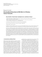
Figure 1: Detection region Ω
T
in sensor coordinate system. Sensors
i and j are in the detection region.
to be searched over the time interval t
0
≤ t ≤ t
0
+ T (hence-
forth referred to as the search interval), and let

x
T
(t)denote
the location of the target at time t. We assume that the tar-
get remains in the search region S and moves with constant
speed V in a fixed direction θ throughout the search interval.
The target track over the search interval is then given by

x
T

t


=

x
T

t
0

+

t − t
0

V

cos θ,sinθ

,(1)
where we recall that t parameterizes the search interval t
0
≤
t ≤ t
0
+ T.Let

x
i
, i = 1, ,N denote the locations in S of
N fixed sensors. We assume the sensors all have identical fi-

nite detection range R
d
and known probability of detection
P
d
. A target detection is defined to occur on sensor i dur-
ing the search interval with probability P
d
if and only if the
target passes within a distance R
d
of the sensor (during that
interval). Define the region Ω
T
as
Ω
T
=


x
∈ R
2
:



x
−


x
T
(t)


≤
R
d
, t
0
≤ t ≤ t
0
+ T

,(2)
where
· denotes Euclidean distance. Hence, if sensor i de-
tects the target during the search interval, then

x
i
∈ Ω
T
.
Moreover, if k sensors detect the target during the search in-
terval, then

x
i
1

, ,

x
i
k
∈ Ω
T
for some subset {i
1
, , i
k
} of
{1, , N}.TheregionΩ
T
, referred to as a “target pill” in [9]
because of its shape, is depicted in Figure 1. This region is the
spatial-temporal coverage, or detection, region for the target.
A natural measure of localization accuracy is the area of
uncertainty, which identifies a region of the search space S
where the target is located. Often, the area of uncertainty is
presented as a collection of closed sets, where each member
of the collection identifies a region of S where the target is lo-
cated with a certain probability. The area of uncertainty pre-
sented in this paper is a single connected closed subset of S
that contains the target with a probability one.
The search coverage region Ω
T
in (2) is defined with re-
spect to a sensor-referenced coordinate system, for which the
area of uncertainty lacks a simple geometrical description.

However, considering the target-referenced coordinate sys-
tem (in which the target is fixed and the sensors move with
constant speed in the opposite direction) provides a mecha-
nism for examining the area of uncertainty over the multiple
(nonsimultaneous) sensor detections in a geometrically in-
tuitive manner, as described below. In this target frame of
T. A. Wettergren and M. J. Walsh 3
R
d
R
d
VT
VT
Ω
i
Ω
j
θ

x
i
(t
0
)

x
i
(t
0
+ T)


x
j
(t
0
)

x
j
(t
0
+ T)

x
T
(t
0
)
Figure 2: Detection regions Ω
i
and Ω
j
in target coordinate system.
At time t
0
,thetargetlocation

x
T
(t

0
) is in the intersection of the
detection regions for sensors i and j.
reference, the target is fixed and the sensors move with speed
V in direction θ + π. The track of sensor i in the target coor-
dinate system over the search interval is then given by

x
i
(t) =

x
i

t
0

+

t − t
0

V

cos(θ + π), sin (θ + π)

=

x
i


t
0

−

t − t
0

V

cos θ,sinθ

.
(3)
Recall that in the sensor coordinate system, if sensor i detects
the target during the search interval, then the target passes
within a distance R
d
of the sensor. Thus, in the target coor-
dinate system, if the target is detected by sensor i during the
search interval, then the sensor passes within R
d
of the target.
For i
= 1, , N,let
Ω
i
=



x
∈ S :



x
−

x
i
(t)


≤
R
d
, t
0
≤ t ≤ t
0
+ T

(4)
represent the region of target detectability about sensor i.
Thus, if sensor i detects the target during the search interval
t
0
≤ t ≤ t
0

+T, then

x
T
(t
0
) ∈ Ω
i
. Furthermore, if the target is
detected by k sensors (e.g., sensors i
1
, , i
k
), then the target
at time t
0
must lie in the intersection of the detection regions
for these sensors, denoted Ω
int
(k), that is,

x
T

t
0

∈

1≤j≤k

Ω
i
j
≡ Ω
int
(k). (5)
This situation is depicted in Figure 2 for the case where the
target is detected by two sensors, labeled i and j.Theregion
of intersection of the two “pills” Ω
i
and Ω
j
is the spatial-
temporal detection region for the target in the target coor-
dinate system.
Let A
Ω
denote the area of the detection region Ω
T
. Since
the transformation between the sensor and target reference
frames is a pure translation, and since the sensor model
is homogeneous in detection characteristics, it follows that
A
Ω
= area(Ω
i
)fori = 1, , N as well. Given k detections,
let A
int

(k) denote the area of intersection of the k detec-
tion regions in the target coordinates, that is, let A
int
(k) =
area(Ω
int
(k)). From the example in Figure 2, it is clear that
A
int
(k) is a complicated function of the sensor locations, the
sensor detection radius, the target initial location, course,
R
d
R
d
2R
d
VTΩ
i
(x
i
, y
i
)
Figure 3: Rectangular coverage region for sensor i in target coordi-
nates.
and speed, and the length of the search interval. However, for
VT
 R
d

, the region Ω
i
,withareaA
Ω
= πR
2
d
+2R
d
VT,is
well approximated by the bounding rectangular region with
dimensions 2R
d
×(2R
d
+ VT), and with area 4R
2
d
+2R
d
VT.
Recall that all sensors translate identically under the transfor-
mation to target coordinates, so all of the bounding rectan-
gles for the different sensors are similarly aligned. Thus the
intersection of any two of these overlapping rectangular de-
tection regions is itself a rectangle with area greater than that
of the intersection of the pills they bound. By induction, the
intersection of any k of these overlapping rectangles, k
≥ 2,
is a rectangle with area greater than that of the intersection

of the k corresponding pills. It follows that the area of inter-
section for the rectangular approximation to the pill-shaped
detection regions is strictly greater than the area of the actual
intersection and, hence, provides a strict upper bound on the
area of uncertainty for track-before-detect systems under the
circular “cookie-cutter” sensor model under consideration.
Throughout the sequel, let Ω
i
, the coverage region of sen-
sor i in the target frame of reference, be the rectangle of
length L
y
= 2R
d
+ VT and width L
x
= 2R
d
. The rectan-
gles are oriented such that the longer axis is parallel to the
direction of target motion, taken here to be, without loss of
generality, θ
= π/2, corresponding to the y-axis. (Extensions
to arbitrary target course θ are obtained by a simple rota-
tion of coordinate axes.) The coverage region Ω
i
is depicted
in Figure 3. Note that the direction of sensor motion in the
target coordinate system is θ + π
= π/2+π = 3π/2. This ge-

ometrical construction leads to Ω
i
={(x, y) ∈ S : x
i
− R
d
≤
x ≤ x
i
+ R
d
, y
i
− VT − R
d
≤ y ≤ y
i
+ R
d
} for any sensor
i
∈{1, , N} that detects the target. With these definitions,
the following lemma provides a formula for the area of inter-
section of these rectangular detection regions in target coor-
dinates given k detections.
Lemma 1. Suppose there are k
≥ 1 regions Ω
i
w ith nonempty
intersection corresponding to detections of a single target dur-

ing the search interval. Without loss of generality, assume the
sensors are labeled such that the detections occur on s ensors
4 EURASIP Journal on Advances in Signal Processing
i ∈{1, , k}.Letd
x
(k) and d
y
(k) be defined as follows:
d
x
(k) = max
1≤i≤k

x
i

− min
1≤i≤k

x
i

,
d
y
(k) = max
1≤i≤k

y
i


−
min
1≤i≤k

y
i

.
(6)
Then A
int
(k), the area of the region of joint intersection Ω
int
(k)
(as defined in (5)), is given by
A
int
(k) =

L
x
−d
x
(k)

L
y
−d
y

(k)

. (7)
Proof. Take any point p
= (u, v)inR
2
. Then p ∈ Ω
int
(k)if
and only if
x
i
−R
d
≤ u ≤ x
i
+ R
d
,
y
i
−VT −R
d
≤ v ≤ y
i
+ R
d
,
(8)
for i

= 1, , k. These inequalities hold if and only if
max
1≤i≤k

x
i

−R
d
≤ u ≤ min
1≤i≤k

x
i

+ R
d
,
max
1≤i≤k

y
i

−VT −R
d
≤ v ≤ min
1≤i≤k

y

i

+ R
d
.
(9)
Since the point p
= (u, v)inR
2
is arbitrary, it follows that
Ω
int
(k) =

max
1≤i≤k

x
i

−R
d
,min
1≤i≤k

x
i

+ R
d


×

max
1≤i≤k

y
i

−VT −R
d
,min
1≤i≤k

y
i

+ R
d

.
(10)
Now,
min
1≤i≤k

x
i

+ R

d
−

max
1≤i≤k

x
i

−R
d

=
min
1≤i≤k

x
i

−
max
1≤i≤k

x
i

+2R
d
= L
x

−d
x
(k).
(11)
Likewise,
min
1≤i≤k

y
i

+ R
d
−

max
1≤i≤k

y
i

−
VT −R
d

=
min
1≤i≤k

y

i

−max
1≤i≤k

y
i

+2R
d
+ VT = L
y
−d
y
(k).
(12)
Thus the area A
int
(k) of the intersection Ω
int
(k)isequalto
(L
x
−d
x
(k))(L
y
−d
y
(k)). Note that for k = 1, d

x
(1) = d
y
(1) =
0, and A
int
(1) = L
x
L
y
= (2R
d
)(2R
d
+VT) = A
Ω
,asexpected.
This lemma explicitly shows that the region of poten-
tial target locations for k detections, Ω
int
(k), and its area,
A
int
(k), are functions of the sensor detection range R
d
, the
sensor locations

x
1

, ,

x
k
, the target speed V, and the length
T of the search interval. Implicitly, Ω
int
(k)andA
int
(k)are
also functions of initial target location

x
T
(t
0
), as the partic-
ular k-subset of N sensors that detect the target obviously
depends on the location of the target in the search space S.
In general, any one of these variables may be random. This
paper is concerned with the statistics of A
int
(k)asafunc-
tion of

x
T
(t
0
) when R

d
, V,andT are fixed and known, and
the sensor locations

x
1
, ,

x
N
are distributed randomly in
S according to a fixed and known, but arbitrary, distribu-
tion function. The explicit computation of the expected value
and variance of A
int
(k)intermsofR
d
, V, T,

x
1
, ,

x
k
,and

x
T
(t

0
) provides a means for representing localization accu-
racy of track-before-detect search strategies in terms of these
important distributed sensor system design parameters.

x
i

x
j
Ω
T

x
T
(t
0
+ T)

x
T
(t
0
)
L
y
(x
Ω
, y
Ω

)
L
x
Figure 4: Rectangular detection region in sensor coordinates.
2.1. Expected value of A
int
(k)
Suppose there are k
≥ 1detectionsonsensorsi = 1, ,k.
Since these sensors detect the target during the search inter-
val, then it must be the case that, in the sensor frame of refer-
ence,

x
1
, ,

x
k
∈ Ω
T
. This situation is depicted in Figure 4,
where only sensors i and j,1
≤ i<j≤ k, are explicitly
labeled. Let x
(1)
, , x
(k)
and y
(1)

, , y
(k)
denote the order
statistics [11] associated with the x and y coordinates, respec-
tively, of the k sensor locations. Lemma 1 gives the area of
intersection A
int
(k) of the detection region Ω
int
(k)asafunc-
tion of the range (the maximum value minus the minimum
value) of the order statistics x
(1)
, , x
(k)
and y
(1)
, , y
(k)
,
that is, d
x
(k) = x
(k)
− x
(1)
and d
y
(k) = y
(k)

− y
(1)
.Weuse
known results on the range of order statistics [11]tocom-
pute the expected value and variance of the area of intersec-
tion A
int
(k).
From Lemma 1, the area of intersection of the detection
regions Ω
1
, , Ω
k
is given by
A
int
(k) = A
Ω

1 −
d
x
(k)
L
x

1 −
d
y
(k)

L
y

, (13)
where A
Ω
= L
x
L
y
is the area of the coverage region Ω
i
of a
single sensor. If the sensor locations are distributed indepen-
dently in x and y, then the expected value of A
int
(k)isgiven
by
E

A
int
(k)

=
A
Ω

1 −
E


d
x
(k)

L
x

1 −
E

d
y
(k)

L
y

. (14)
The sensor locations within the search region S are assumed
to be random, with a fixed and known distribution function.
Let F(x, y) represent the distribution function correspond-
ing to the random locations of the sensors. The correspond-
ing density function f (x, y)isgivenby f
= F

. Furthermore,
let f
X
and f

Y
represent the marginal density functions of the
sensor locations in the x and y coordinates, respectively, with
associated distribution functions F
X
and F
Y
. Since the ranges
d
x
(k)andd
y
(k) depend on the locations of the detecting sen-
sors, the expected values E(d
x
(k)) and E(d
y
(k)) clearly de-
pend on these distribution functions. In particular, from the
T. A. Wettergren and M. J. Walsh 5
theory of order statistics (see Stuart and Ord [11, page 495]),
the expected value of d
x
(k)isgivenby
E

d
x
(k)


=

x
Ω
+L
x
x
Ω

1 −

F
X|Ω
T
(x)

k
−

1 − F
X|Ω
T
(x)

k

dx,
(15)
where F
X|Ω

T
and F
Y|Ω
T
represent the conditional distribution
functions for F
X
and F
Y
, respectively, conditioned on the de-
tection region Ω
T
.Equation(15)isderivedin[11]bysub-
stituting the well-known density functions for the minimum
and maximum order statistics x
(1)
and x
(k)
into the identity
E(d
x
(k)) = E(x
(k)
) − E(x
(1)
), and using integration by parts
to simplify the resulting expression. A similar expression to
(15) holds for the expected value of the range d
y
(k).

The conditional distribution function F
X|Ω
T
is given by
F
X|Ω
T
(x) =
⎧
⎪
⎪
⎪
⎪
⎨
⎪
⎪
⎪
⎪
⎩
0, x<x
Ω
,

x
x
Ω
f
X|Ω
T
(ξ)dξ, x

Ω
≤ x ≤ x
Ω
+ L
x
,
1, x>x
Ω
+ L
x
,
(16)
where the point (x
Ω
, y
Ω
) denotes the lower left-hand corner
of Ω
T
(see Figure 4), and
f
X|Ω
T
(x) =
f
X
(x)

x
Ω

+L
x
x
Ω
f
X
(ξ)dξ
, x
Ω
≤ x ≤ x
Ω
+ L
x
, (17)
and similarly for F
Y|Ω
T
and f
Y|Ω
T
. Thus, for a known distri-
bution on the sensor locations, the expected value of the area
of the target location region is computed from (14), (15), and
(16) (including the corresponding expressions for E(d
y
(k))
and F
Y|Ω
T
(y)).

If the sensor locations are not distributed independently
in x and y, the expectation operator does not, in general, dis-
tributeacrosstermsinA
int
(k)by(14). However, in practice,
we expect long, narrow detection regions, which is the case
for VT
 R
d
.Foratargetwithcourseθ = π/2, this trans-
lates to a detection region Ω
T
with L
y
 L
x
.Also,forasearch
region S much larger than the detection region Ω
T
,weex-
pect the variation in f
X|Ω
T
over the interval x
Ω
≤ x ≤ x
Ω
+L
x
to be small for all values of x

Ω
. With these assumptions, the
sensor x and y locations are distributed approximately inde-
pendently in Ω
T
, with sensor x location approximately uni-
formly distributed in this region, yielding
f
X|Ω
T
(x) =
⎧
⎪
⎪
⎨
⎪
⎪
⎩
1
L
x
, x
Ω
≤ x ≤ x
Ω
+ L
x
,
0, otherwise,
(18)

which greatly simplifies the evaluation of (15).
2.2. Variance of A
int
(k)
The variance of the area of intersection of the detection re-
gions Ω
1
, , Ω
k
,denotedvar(A
int
(k)), is given by
var

A
int
(k)

= E


A
int
(k) −E

A
int
(k)

2


=
E


A
int
(k)

2

−

E

A
int
(k)

2
,
(19)
where E(A
int
(k)) is given by (14). As in the previous section,
the sensor x and y locations are approximately independent
(within the local region Ω
T
), leading to
E



A
int
(k)

2

=
A
2
Ω
E


1 −
d
x
(k)
L
x

2

E


1 −
d
y

(k)
L
y

2

,
(20)
where
E


1 −
d
x
(k)
L
x

2

=
1 − 2
E

d
x
(k)

L

x
+
E

d
2
x
(k)

L
2
x
= 1 −2
E

d
x
(k)

L
x
+

E

d
x
(k)

2

+var

d
x
(k)

L
2
x
=

1 −
E

d
x
(k)

L
x

2
+
var

d
x
(k)

L

2
x
,
(21)
and similarly for the d
y
(k) term. The expected value of the
range d
x
(k)isgivenby(15); a similar expression gives the ex-
pected value of the range d
y
(k). The variances of the ranges
d
x
(k)andd
y
(k) are found using known results on order
statistics. From [11, page 495],
var

d
x
(k)

=
2

x
Ω

+L
x
x
Ω

x
(n)
x
Ω

1 −

F
X|Ω
T

x
(n)

k
−

1 − F
X|Ω
T

x
(1)

k

+

F
X|Ω
T

x
(n)

−
F
X|Ω
T
(x
(1)
)

k

dx
(1)
dx
(n)−(E(d
x
(k)))
2
(22)
for k
≥ 1, and similarly for var(d
y

(k)).Thechangeofvari-
ables u
= x
(k)
, v = (x
(1)
−x
Ω
)/(x
(k)
−x
Ω
) replaces the iterated
integral in (22) by one with constant limits of integration,
yielding
var

d
x
(k)

=
2

x
Ω
+L
x
x
Ω


1
0

1 −

F
X|Ω
T
(u)

k
−

1 − F
x|Ω
T

(1 − v)x
Ω
+ uv

k
+

F
X|Ω
T
(u) − F
X|Ω

T

(1 − v)x
Ω
+ uv

k

×

u − x
Ω

dv du
−

E

d
x
(k)

2
(23)
for k
≥ 1, and similarly for var(d
y
(k)). These latter expres-
sions for the variances of the ranges d
x

(k)andd
y
(k) are more
amenable to numerical evaluation, and are used for the ex-
amples in Section 4.
Observe that for k
= 1, (22)and(23)yieldvar(d
x
(1)) =
0. Substituting this result into (21)givesE((1−d
x
(1)/L
x
)
2
) =
1, and substituting this result into (20)givesE((A
int
(1))
2
) =
A
2
Ω
. It then follows from (19) that var(A
int
(1)) = 0. This re-
sult is expected, since given a singledetection from sensor i,
6 EURASIP Journal on Advances in Signal Processing
the area of uncertainty is precisely the area of the detection

region Ω
i
(equivalently, the detection region Ω
T
).
2.3. Uniform sensor distribution
Given the general expressions for the expected value and
variance of A
int
(k), we now examine the special cases when
sensor location is distributed according to the uniform distri-
bution in one or both coordinates. In the latter case, the ex-
pected value and variance of A
int
(k) take simple closed forms.
As described in Section 2.1, the case of sensors uniformly dis-
tributed in x is a general assumption considered in practice.
This assumption leads to simplification based on the follow-
ing lemma.
Lemma 2. Suppose the sensor x locations are distributed
uniform(x
Ω
, x
Ω
+L
x
) in Ω
T
. Then d
x

(k)/L
x
has mean and vari-
ance given by
E

d
x
(k)
L
x

=
E

d
x
(k)

L
x
=
k − 1
k +1
,
var

d
x
(k)

L
x

=
var

d
x
(k

L
2
x
=
2(k − 1)
(k +1)
2
(k +2)
,
(24)
respectively. Moreover, d
x
(k)/L
x
is distributed beta(k − 1, 2).
The detailed proof of Lemma 2 is given in the appendix.
Incidentally, this lemma holds equally for sensors with y lo-
cations distributed uniform(y
Ω
, y

Ω
+ L
y
). This observation
leads to the following theorem.
Theorem 1. If sensor x and y locat ions are distributed inde-
pendently and uniformly in Ω
T
, then
E(A
int
(k)) =
4A
Ω
(k +1)
2
, (25)
var

A
int
(k)

=
4

5k
2
+2k − 7


A
2
Ω
(k +1)
4
(k +2)
2
. (26)
Proof. Since the sensors are assumed distributed uniformly
in x and y, Lemma 2 gives
E

d
x
(k)

L
x
=
E

d
y
(k)

L
y
=
k − 1
k +1

. (27)
Substituting this result into (14) yields
E

A
int
(k)

=
A
Ω

1 −
k − 1
k +1

2
=
4A
Ω
(k +1)
2
. (28)
Since d
x
(k)andd
y
(k) are independent and identically dis-
tributed, (19), (20), and (21)yield
var


A
int
(k)

=
A
2
Ω


1 −
E

d
x
(k)

L
x

2
+
var(d
x
(k))
L
2
x


2
−

E

A
int
(k)

2
.
(29)
Substituting the expressions for E(d
x
(k)) and var(d
x
(k)) as
given in Lemma 2, along with (25)forE(A
int
(k)) gives
var

A
int
(k)

=
36A
2
Ω

(k +1)
2
(k +2)
2
−
16A
2
Ω
(k +1)
4
=
4

5k
2
+2k − 7

A
2
Ω
(k +1)
4
(k +2)
2
.
(30)
We note that Theorem 1 shows that the localization accu-
racy depends only upon the area of the detection region Ω
T
and the number of detections k; it does not explicitly depend

on the number of sensors nor sensor density. However, there
is an implicit dependence on these quantities since obtaining
k detections requires a minimal number of sensors, as shown
in [9].
3. DISTRIBUTION OF A
int
(k) GIVEN k ≥ 
The quantities E(A
int
(k)) and var(A
int
(k)) represent the ex-
pected value and variance, respectively, of the area of the un-
certainty region Ω
int
(k), given k detections. When a sensor
field is deployed and operating, the number of detections k
is itself a random variable and, like A
int
(k), is a function of
the sensor locations and detection characteristics, the target
kinematics, and the search interval. The distribution func-
tion for k as a function of these variables is given by Wetter-
gren in [9]. This probability distribution is used to obtain the
expected value and variance of the area of uncertainty given
at least  detections, that is, given k
≥ .
Let K denote the random variable associated with the ob-
served number of detections k. Then the probability of get-
ting k detections is denoted P(K

= k), the probability of get-
ting at least one detection is denoted P(K
≥ 1), and so on.
Incidentally, the probability of getting at least k detections,
P(K
≥ k), is referred to in [9]asthe(systemlevel)proba-
bility of successful search, and is also denoted by P
SS
(k). A
successful search is defined in [9] as the event of obtaining at
least k detections for some prescribed value of k; this event
occurs with probability P
SS
(k).
The probability of getting exactly k detections, as well as
the system level probability of successful search P
SS
(k), de-
pends on the sensor level probability of successful search, de-
noted p in [9]. This probability is defined as
p
= 1 −exp

−P
d
ϕ

, (31)
where P
d

is the (apriori) sensor probability of detection, and
ϕ is the probability of finding a sensor in the spatial-temporal
target detection region Ω
T
, that is,
ϕ
=

Ω
T
f


x

d

x, (32)
T. A. Wettergren and M. J. Walsh 7
where f is the sensor location density function. The event
of getting exactly k detections is defined in terms of the out-
come of N independent Bernoulli trials (N being the total
number of sensors), with success probability p,asgivenby
(31), and failure probability 1
− p. Then the resulting distri-
bution function for the number of observed detections k is
given by the binomial distribution
P(K
= k) =


N
k

p
k
(1 − p)
N−k
, k = 0, 1, , N. (33)
The corresponding conditional distribution function P(K
=
k | K ≥ )isgivenby
P(K
= k | K ≥ ) =
⎧
⎪
⎪
⎪
⎪
⎨
⎪
⎪
⎪
⎪
⎩
0, if k<,
P(K
= k)
1 −

0≤i<

P(K = i)
,ifk
≥ .
(34)
Let E(A
int
| ) = E(A
int
(K) | K ≥ ) denote the ex-
pected value of A
int
(k) given at least  detections. Likewise,
let var(A
int
| ) = var(A
int
(K) | K ≥ ) denote the variance
of A
int
(k)givenk ≥ . Then
E

A
int
| 

=

0≤k≤N
E(A

int
(k))P(K = k | K ≥ ),
var

A
int
| 

=

0≤k≤N
var(A
int
(k))P(K = k | K ≥ ),
(35)
where E(A
int
(k)) and var(A
int
(k)) are given, in general, by
(14)and(19), respectively.
Finally, as pointed out by Wettergren in [9], binomial
probabilities such as (33)and(34)aredifficult to evaluate
numerically for even moderate numbers of sensors because
of the N! term in the binomial coefficient. However, the size
of the detection region Ω
T
is typically small compared to the
size of the search space S so that the probability ϕ of finding
a sensor in Ω

T
is much less than one. Thus, for P
d
< 1, we
have, from (31), that p
≈ 1 − (1 − P
d
ϕ) = P
d
ϕ.Hence,for
ϕ
 1, we conclude that p  1. For N  1, the DeMoivre-
Laplace theorem [12] provides an approximate evaluation of
the binomial coefficient. In the case of N
 1andp  1,
the distribution of Bernoulli trials is well-approximated by
the limiting case of the Poisson theorem, yielding
P(K
= k) =

N
k

p
k
(1 − p)
N−k
≈
(Np)
k

k!
exp (
−Np), (36)
(see Feller [12, Chapter 6, Section 5]). As an example of the
use of this approximation, substituting the approximation
into expression (34) for the conditional probability of get-
ting k detections, having gotten at least one (
= 1) detection,
gives
P(K
= k | K ≥ 1)
≈
1
1 −

1 − P
d
ϕ

N

NP
d
ϕ

k
k!
exp

−

NP
d
ϕ

,1≤ k ≤ N,
(37)
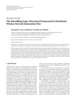
10.80.60.40.20
E(A
int
)/A
Ω
0
0.1
0.2
0.3
0.4
0.5
0.6
0.7
0.8
0.9
1
P(K ≥ 1)
Increasing N
Figure 5: Probability of receiving a detection versus expected local-
ization accuracy.
where the probability of receiving at least one detection is
P(K
≥ 1) = 1 −(1 − P
d

ϕ)
N
.
In Figure 5, the probability of receiving at least one de-
tection is plotted versus the expected value of the area of in-
tersection for a set of sensors uniformly distributed over the
search region. For convenience, the expected area of inter-
section is normalized by the single detection area A
Ω
.The
curve in the figure is parameterized by the density of sensors
in the search region (or, equivalently, the number of sensors
N). When there are very few sensors, the probability of de-
tection is small, and when detection occurs, it is usually only
a single sensor detection and thus the expected area of inter-
section corresponds to the detection region of a single sen-
sor (since E(A
int
(1)) = A
Ω
). Thus the normalized expected
area of intersection approaches unity for small numbers of
sensors. As the number of sensors increases, the likelihood
of receiving more than one detection in the search interval
increases, thus increasing the probability of at least one de-
tection (P(K
≥ 1)), as well as decreasing the expected area
of intersection due to the reduction in the size of the in-
tersection region with increasing numbers of detections (see
(25)). The expected detection and localization performance

of a distributed sensor field design can thus be set by care-
fully considering these relationships when determining the
density of sensors to employ in the field.
4. LOCALIZATION EXAMPLES
In this section, we examine the localization accuracy of the
track-before-detect search strategy described in [9]foratar-
getwithspeedV
= 1 moving in direction θ = π/2 through
asearchspaceS
= [−10, 10] ×[−10, 10] covered by a field of
N
= 50 sensors, each with detection range R
d
= 1, and over a
search interval of duration T
= 5. In particular, the mean and
variance of the area of uncertainty A
int
(k) given at least one
detection are examined as functions of target location at the
midpoint of the detection region Ω
T
. These example calcu-
lations are performed for three random sensor distributions:
8 EURASIP Journal on Advances in Signal Processing
a uniform distribution, a barrier distribution, and an arbi-
trary distribution.
Note that for this example, the area A
Ω
of the detection

regions Ω
T
and {Ω
i
}
1≤i≤k
is equal to 4R
2
d
+2R
d
VT = 4+
2
·5 = 14. Then, for k = 1, we have
E(A
int
(K) | K = 1) = A
Ω
= 14, var(A
int
(K) | K = 1) = 0.
(38)
Furthermore, in regions of S for which the sensor location
density function has little support, we have P(K
= k | K ≥
1) ≈ 0forall1<k≤ N. In these regions, (35)imply
E

A
int

| 1

≈
A
Ω
= 14, var

A
int
| 1

≈
0. (39)
These observations are illustrated in the examples of Sections
4.2 and 4.3. The sensor location density functions for the ex-
amples in these sections have near zero support in large re-
gions of the search space S.
4.1. Uniform sensor field
We first consider the 50 sensors distributed in S according
to the uniform distribution function, that is, the sensor x
and y locations are independently and identically distributed
uniform(
−10, 10). Substituting the results of Theorem 1 into
expressions (35), the expected value and variance of A
int
(k)
given at least one detection are given by the following:
E

A

int
| 1

=
4A
Ω
1 −

1 − P
d
ϕ

N

1≤k≤N

NP
d
ϕ

k
(k +1)(k +1)!
exp

−
NP
d
ϕ

,

var

A
int
| 1

=
4A
2
Ω
1 −

1 − P
d
ϕ

N

1≤k≤N

5k
2
+2k − 7

NP
d
ϕ

k
(k +1)

3
(k +2)(k +2)!
× exp

−
NP
d
ϕ

.
(40)
Theseanalyticalresultsareverifiedexperimentallybyes-
timating E(A
int
| 1) and var(A
int
| 1) from a sequence of
random draws of 50 sensors from the uniform distribution
function on the search space S. In particular, consider the de-
tection region Ω
T
centered at the origin of S.Form random
draws of 50 sensors, let m
k
be the number of times k sensors
are in the region Ω
T
for k = 0, 1, , 50. For the ith draw out
of m draws, if the number of detections k>0, set A
i

(k)equal
to A
int
(k), computed using expression (7). Given m random
draws, the probability of getting k detections given k
≥ 1is
estimated by
P(k) =
m
k
/m
1 − m
0
/m
=
m
k
m − m
0
, (41)
and the mean and variance of the area of intersection given k
detections are estimated by the sample statistics
A
int
(k)and
V
int
(k), respectively, as given by
A
int

(k) =
1
m

1≤i≤m
A
i
(k),
V
int
(k) =
1
m

1≤i≤m

A
i
(k) −A
int
(k

2
.
(42)
The estimated mean and variance of A
int
(k) given at least one
detection, denoted
A

int
and V
int
,respectively,arecomputed
by combining these results, as in (35):
A
int
=

1≤k≤N
P(k)A
int
(k), V
int
=

1≤k≤N
P(k)V
int
(k).
(43)
Figures 6(a) and 6(b) show box plots of 300 values of
A
int
and V
int
, where each pair of values is estimated from
m
= 100 and m = 1000 samples of 50 sensors, respectively.
The top and bottom lines of each box represent the upper and

lower quartile values of the sample, and the line in-between
these two lines represents the sample median; the dashed
lines (“whiskers”) extending from the top and bottom of each
box represent the spread of the remaining sample, and any
plus signs beyond the whiskers represent outliers. The true
values E(A
int
| 1) = 8.1540 and var(A
int
| 1) = 4.6338 for
this example, computed using (40), are indicated in these
plots by asterisks. Clearly, the uncertainty in our estimates
of E(A
int
| 1) and var(A
int
| 1) decreases with an increase in
the number of 50-sensor samples, from 100 to 1000, over the
300 experiments.
4.2. Sensor barrier
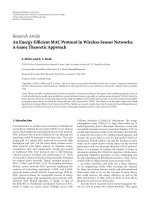
Now, consider a nonuniform sensor distribution in the
search region S in which the sensors are distributed in the
x and y dimensions according to the uniform and nor-
mal distribution functions, respectively. Specifically, con-
sider the sensor x locations distributed independently
uniform(
−10, 10), and the sensor y locations distributed in-
dependently normal(μ, σ)withmeanμ
= 0 and standard de-
viation σ

= 2. Contours of the joint density function f
XY
are
plotted in Figure 7, along with a sample of 50 sensors. This
distribution forms a natural barrier against targets moving
across the line y
= μ; hence, we refer to it as a barrier distri-
bution.
The expected value and variance of the area of uncer-
tainty A
int
, given at least one detection, are found using the
results of Sections 2.1, 2.2,and3. These results require the
conditional distribution functions F
X|Ω
T
(x)andF
Y|Ω
T
(y).
For sensors distributed independently uniform(
−10, 10) in
the x dimension, we have f
X|Ω
T
(x) = 1/L
x
, which gives
F
X|Ω

T
(x) = (x − x
Ω
)/L
x
for x restricted to Ω
T
.Letφ denote
the standard normal density function (with zero mean and
standard deviation one), and let Φ denote its distribution
function, so that, for
−∞ <t<∞,
ϕ(t) =
1
√
2π
exp

−t
2
/2

,
Φ(t)
=

t
−∞
φ(τ)dτ =
1

2

1+erf

t/
√
2

.
(44)
T. A. Wettergren and M. J. Walsh 9
var(A
int
)E(A
int
)
2
3
4
5
6
7
8
9
10
Va lu e
(a) Estimated from 100 50-sensor samples
var(A
int
)E(A

int
)
4
4.5
5
5.5
6
6.5
7
7.5
8
8.5
Va lu e
(b) Estimated from 1000 50-sensor samples
Figure 6: Box plots of 300 experimental values of E(A
int
| 1) and
var(A
int
| 1), each pair estimated from (a) 100 and (b) 1000 samples
of 50 sensors. The asterisks indicate the analytical values E(A
int
|
1) = 8.1540 and var(A
int
| 1) = 4.6338 given by (40), respectively.
It follows that, for sensors distributed independently
normal(μ, σ) in the y dimension, we have, for y restricted
to Ω
T

,
f
Y|Ω
T
(y) =
1
cσ
φ

y − μ
σ

, (45)
with normalization constant c given by
c
= Φ

y
Ω
+ L
y
−μ
σ

−
Φ

y
Ω
−μ

σ

. (46)
Consequently, the conditional distribution function F
Y|Ω
T
for this example is given by
F
Y|Ω
T
(y) =
1
c

Φ

y − μ
σ

−
Φ

y
Ω
−μ
σ

. (47)
1050−5−10
x

−10
−8
−6
−4
−2
0
2
4
6
8
10
y
Figure 7: Sensor location density function for the barrier example,
with N
= 50 sampled sensors.
Since the sensor locations are distributed independently
in the x and y dimensions, and, moreover, uniformly in the
x dimension, the expected values and variances of A
int
(k)
and A
int
are independent of sensor x location. Figure 8
shows plots of E(A
int
| 1) (solid line) and var(A
int
| 1)
(dashed line) for the midpoint of the target track at y
=

−
6.5, −5.5, ,5.5, 6.5. The endpoints −6.5 and 6.5 are cho-
sen so that the bottom and top of the detection region Ω
T
about the target track coincide with the bottom and top, re-
spectively, of the search space S. The theoretical curves in
Figure 8 are verified experimentally by estimating E(A
int
| 1)
and var(A
int
| 1) using the same approach as in the previous
example. In this example, instead of estimating the sample
statistics
A
int
and V
int
for m = 1000 50-sensor draws and for
the detection region Ω
T
centered at the origin of S,wecom-
pute these statistics for m
= 1000 50-sensor draws and for
the sensor detection region Ω
T
centered at x = 0andeachof
the locations y
=−6.5, −5.5, ,5.5,6.5. For each of these 14
locations of the detection region Ω

T
on the y-axis, 19 values
of
A
int
and V
int
are plotted in Figure 8 as circles and crosses,
respectively. These estimates show good agreement with the
theoretical curves.
The analytical and experimental results in Figure 8 show
some interesting trends. That the expected area of intersec-
tion, or area of uncertainty, should decrease monotonically
as the target enters the sensor barrier, and then increase at
the opposite rate as the target leaves the barrier, is intu-
itively obvious, given the symmetry of this example. Few, if
any, detections are expected in the tails of the barrier; it fol-
lows that the expected value of the area of uncertainty given
at least one detection is essentially equal to the area of the
detection region Ω
T
in these regions of S (recall that area
(Ω
T
) = A
Ω
= 14, for this example). Likewise, the area of un-
certainty should be minimum in the region of S with densest
10 EURASIP Journal on Advances in Signal Processing
14121086420

Va lu e
−8
−6
−4
−2
0
2
4
6
8
y
Mean
Va ri an ce
Figure 8: Expected value and variance of area of intersection given
at least one detection, as functions of the y location of the midpoint
of the detection region Ω
T
, for the barrier example.
sensor coverage, which, for this example, is the line y = 0. In-
deed, the expected area of uncertainty given at least one de-
tection for this example reaches its minimum value of 3.5552
at y
= 0.
On the other hand, the behavior of the variance of the
area of uncertainty for this example, as displayed by the
dashed line in Figure 8, is not so clearly anticipated. In the
tails of the barrier, where few, if any, detections are expected,
the variance of the area of uncertainty given at least one de-
tection tends to zero as the target moves away from the bar-
rier. This result is expected, since given exactly one detection,

the variance is precisely zero. That the variance should in-
crease as the target enters the barrier is also reasonable, as
the uncertainty in the area of intersection A
int
(k) necessarily
increases (from zero) once more than one sensor contributes
to the region of intersection Ω
int
(k), that is, for k>1. How-
ever, as the target approaches the center of the barrier, where
the sensor density is greatest, the variance of the area of un-
certainty decreases, and reaches its minimum value of 3.4601
at y
= 0. Evidently, for this example, there is a value of sensor
density that, when exceeded, yields a decrease in the variance
of the area of uncertainty, and otherwise leads to an increase
in this variance.
4.3. Arbitrary sensor field
As a next example, consider sensors distributed randomly ac-
cording to an arbitrary distribution function, and in partic-
ular, one for which the distributions of the x and y sensor
locations are dependent. In this case, given the assumptions
presented at the end of Section 2.1, that is, for a long, narrow
detection region Ω
T
, and for a sensor location density func-
tion f
XY
that does not vary much in the x dimension (the
narrow dimension of Ω

T
), it is reasonable to assume that the
sensor x and y locations are locally independent in Ω
T
,so
that
f
XY|Ω
T
(x, y) ≈ f
X|Ω
T
(x) f
Y|Ω
T
(y), (48)
with the conditional density function f
X|Ω
T
given by (18)and
f
Y|Ω
T
given by
f
Y|Ω
T
(y) =
f
XY


X = x
Ω
+ L
x
/2, y


y
Ω
+L
y
y
Ω
f
XY

X = x
Ω
+ L
x
/2, ψ

dψ
, (49)
for y
Ω
≤ y ≤ y
Ω
+ L

y
,and f
Y|Ω
T
(y) = 0 otherwise. For
convenience in this example, we use the fact that an arbitrary
density function can be approximated to an arbitrary level of
accuracy by a mixture density function (a weighted sum of
density functions) with a sufficient number of terms. In par-
ticular, consider the K component, heterogeneous, bivariate
normal mixture density function given by
f
XY
(x, y) =
1
K

1≤κ≤K
1
η
κ
φ

x −ν
κ
η
κ

1
σ

κ
φ

y − μ
κ
σ
κ

, (50)
with component means ν
κ
and μ
κ
in the x and y dimensions,
respectively, with corresponding standard deviations η
κ
and
σ
κ
,forκ = 1, , K. Clearly, the x and y components of this
density function are dependent. Given this mixture approxi-
mation to the density function f , and given the assumptions
on the detection region Ω
T
stated above, the conditional den-
sity function f
Y|Ω
T
,asgivenby(49), becomes
f

Y|Ω
T
(y) =
1
c

1≤κ≤K
1
η
κ
φ

x
Ω
+ L
x
/2 −ν
κ
η
κ

1
σ
κ
φ

y − μ
κ
σ
κ


,
(51)
with normalization constant c given by
c
=

1≤κ≤K
1
η
κ
φ

x
Ω
+ L
x
/2 −ν
κ
η
κ

×

Φ

y
Ω
+ L
y

−μ
κ
σ
κ

−
Φ

y
Ω
−μ
κ
σ
κ


.
(52)
The conditional distribution function F
Y|Ω
T
(y)fory
Ω
≤ y ≤
y
Ω
+ L
y
is obtained by integrating (51)fromy
Ω

to y yielding
F
Y|Ω
T
(y) =
1
c

1≤κ≤K
1
η
κ
φ

x
Ω
+ L
x
/2 −ν
κ
η
κ

×

Φ

y − μ
κ
σ

κ

−
Φ

y
Ω
−μ
κ
σ
κ


.
(53)
Substituting (53), and the conditional distribution function
F
X|Ω
T
(x) = (x − x
Ω
)/L
x
for x restricted to Ω
T
, into the results of Sections 2.1, 2.2,
and 3, gives expressions for the expected value and variance
of the area of uncertainty A
int
for an arbitrary, but known,

sensor location distribution function.
T. A. Wettergren and M. J. Walsh 11
Figure 9 shows contours of an arbitrary sensor location
density function, generated using the mixture density func-
tion (50)withK
= 5 components, each with equal x and
y standard deviations η
κ
= σ
κ
= 2forallκ,andwithx
and y mean locations chosen randomly and independently
from the uniform(
−10, 10) distribution. Also shown in this
figure is a sample of 50 sensors. To examine the behavior of
the area of uncertainty for the constant velocity target of the
previous examples for this particular sensor location den-
sity function, we evaluate the expected area of uncertainty,
E(A
int
| 1), and the variance of this area, var(A
int
| 1),
given at least one detection, for the midpoint of the target
track at x
=−9, −8, ,8,9andy =−6.5, −5.5, ,5.5, 6.5.
The points in this rectangular grid are chosen so that the
union of the detection regions Ω
T
centered at each point of

the grid equals the search space S. Figures 10(a) and 11(a)
show the expected value and variance, respectively, of the
area of uncertainty given at least one detection from 50 sen-
sors distributed according to the density function shown in
Figure 9. These quantities are calculated at each point of the
grid using the conditional sensor location distribution func-
tions given above, and the expressions for E(A
int
| 1) and
var(A
int
| 1) derived in Sections 2 and 3. These theoretical
results are verified experimentally by estimating E(A
int
| 1)
and var(A
int
| 1) using the same approach used in the pre-
vious two examples. In particular, we estimate the sample
statistics
A
int
and V
int
for m = 1000 50-sensor draws and
for the detection region Ω
T
centered at each grid point. For
each of the 19
·14 = 266 locations of the detection region Ω

T
in the search region S, the values of A
int
and V
int
are plotted
in Figures 10(b) and 11(b), respectively. For reference, each
of the plots in Figures 10 and 11 show the same sample of
50 sensors shown in Figure 9. Also, each of these plots shows
the target detection region Ω
T
centered at the grid point with
the smallest area of uncertainty, that is, the smallest value of
E(A
int
); the dashed lines indicate the boundary of Ω
T
,and
the arrow represents the target track over the search interval
T.
As for the previous two examples, the estimates
A
int
and
V
int
show good agreement with the corresponding theoreti-
cal values of E(A
int
| 1) and var(A

int
| 1). Also, the general
trends in the expected value and variance of the area of un-
certainty for this arbitrary sensor location distribution are
similar to those observed for the sensor barrier. In particular,
the expected area of uncertainty tends to decrease monoton-
ically as the target approaches regions of dense sensor cov-
erage, and increase monotonically as the target leaves these
regions. Also, while there is an initial increase in the variance
of the area of uncertainty as the target approaches regions
of dense sensor coverage, the variance then decreases when a
certain level of sensor density is exceeded. Both trends have
been consistently observed for other arbitrary sensor loca-
tion distributions generated from the general mixture den-
sity (50), but those results are not included here.
We finally consider a case of a sensor field with >1re-
quired detections. Using an increased value of  in a field de-
sign may be performed to reduce the impact of false alarms
in large fields, as pointed out in [9]. We consider a sensor
field of 50 sensors randomly distributed according to the
1050−5−10
x
−10
−8
−6
−4
−2
0
2
4

6
8
10
y
Figure 9: Arbitrary sensor location density function, with N = 50
sampled sensors.
same process as the previous example. The resulting field is
shown in Figure 12. As in the previous example, we examine
the behavior of the area of uncertainty for the constant ve-
locity target for this particular sensor location density func-
tion. However, in this case, we evaluate the expected value of
the area of uncertainty given at least four detections, that is,
E(A
int
| 4). The points in this rectangular grid are chosen in
the same manner as for Figure 10. Figure 13 shows E(A
int
| 4)
from 50 sensors distributed according to the density func-
tion shown in Figure 12. Note that the expected area is very
small throughout much of the region, with an average that
is noticeably smaller than the previous example (which had
the same number of sensors, but only required a single de-
tection). This is due to the ability of the track-before-detect
kinematic requirements to ignore many detections that are
not aligned with three other detections (for this 
= 4case).
The drawback is that it is not very likely to obtain multi-
ple detections that provide such track information. Figure 14
shows the corresponding probability of obtaining four detec-

tions consistent with the track-before-detect criteria for this
example. It is clear from the figure that the regions of highest
sensor density contain both the highest probability of obtain-
ing multiple detections and the best corresponding expected
area of uncertainty. Unfortunately, as pointed out in previ-
ous work [9], these regions of high sensor density also corre-
spond to the greatest probability of false search results. There
are also many regions in Figure 13 that indicate very good
localization accuracy but are very unlikely to receive the nec-
essary detections (such as the region near (x, y)
= (−4, 1)).
While the preceding examples show that increased sen-
sor density (i.e., clustering of sensors) may be beneficial
to improving localization accuracy, it is important to con-
sider this design objective in the context of other objectives.
In particular, as the last example shows, better localization
12 EURASIP Journal on Advances in Signal Processing
2
2
4
4
4
4
6
6
6
6
6
8
8

8
8
8
8
10
10
10
10
10
10
12
12
12
12
12
1050−5−10
x
−10
−8
−6
−4
−2
0
2
4
6
8
10
y
2

4
6
8
10
12
(a) Analytical result
2
2
4
4
4
4
4
6
6
6
6
6
8
8
8
8
8
8
10
10
10
10
10
10

12
1
2
12
12
12
14
14
14
14
14
1050−5−10
x
−10
−8
−6
−4
−2
0
2
4
6
8
10
y
2
4
6
8
10

12
(b) Experimental result
Figure 10: Expected area of intersection given at least one detec-
tion.
accuracy often comes at the same locations as increased
search effectiveness, but sometimes comes at locations of
poor search effectiveness. Neither having good localization
accuracy without detections nor having many detections
without a sufficiently small area of uncertainty is useful. Even
when we have both good search effectiveness and good lo-
calization, it is often due to a high density of sensors, which
causes more false search reports. Thus we expect these results
to be used in careful tradeoff analyses (as in [13]) to deter-
mine the best tradeoff under design constraints within each
specific deployment scenario.
5. CONCLUSIONS
In this paper, expressions were derived for the expected value
and variance of the area of uncertainty achieved by employ-
ing a track-before-detect search strategy for localizing a tar-
get moving across a distributed sensor network. The analyt-
0.5
0.5
0.
5
0.5
0.
5
1
1
1

1
1
1. 5
1.5
1. 5
1.
5
1.5
1.5
1.5
2
2
2
2
2
2
2
2.5
2.5
2.5
2.5
2.
5
2.
5
2.
5
3
3
3

3
3
3
3
3
3
3.5
3.
5
3.5
3.
5
3.5
3.5
3.5
3. 5
3. 5
3.
5
4
4
4
4
4
4
4
4
4
4
4

4.5
4.5
4.5
4.
5
4.5
4.5
4.5
4.5
4.5
4.5
4.
5
5
5
5
5
5
5
1050−5−10
x
−10
−8
−6
−4
−2
0
2
4
6

8
10
y
0.5
1
1.5
2
2.5
3
3.5
4
4.5
5
(a) Analytical result
0.5
0.5
0.5
0.5
0.5
1
1
1
1
1
1.5
1.5
1.5
1.5
1.5
1. 5

1.5
2
2
2
2
2
2
2
2.5
2.5
2.5
2.5
2.
5
2.
5
2. 5
2.5
3
3
3
3
3
3
3
3
3
3
3.5
3.5

3.5
3.5
3.5
3.5
3.5
3.5
3.
5
3.5
4
4
4
4
4
4
4
4
4
4
4
4. 5
4.5
4.
5
4.5
4. 5
4.5
4.5
4.5
4.5

4.5
4.5
5
5
5
5
5
5
5
1050−5−10
x
−10
−8
−6
−4
−2
0
2
4
6
8
10
y
0.5
1
1.5
2
2.5
3
3.5

4
4.5
5
(b) Experimental result
Figure 11: Variance of area of intersection given at least one detec-
tion.
ical expressions were verified by comparison with computa-
tional experiments. Examples of uniform, barrier, and arbi-
trary field designs were analyzed using these expressions. By
studying the analytical expressions for localization accuracy,
system designers can develop apriorimeasures of effective-
ness of the resulting sensor system in a parametric manner,
thus enabling the optimal setting of critical design parame-
ters, such as the placement of sensors within a search area.
The analytical nature of these expressions further provides a
mechanism for rapid assessment of the area of uncertainty
for systems operating in real-time, which is beneficial in as-
sessing the potential impact of field degradation on system
performance. The use of these expressions within tradeoff
analyses for distributed sensor system design is a subject of
on-going research.
The present paper is concerned with track-before-detect
that is limited to kinematic matching of expected target be-
havior to sensor detections. By considering the expected
T. A. Wettergren and M. J. Walsh 13
1050−5−10
x
−10
−8
−6

−4
−2
0
2
4
6
8
10
y
Figure 12: A second arbitrary sensor location density function,
with N
= 50 sampled sensors.
1. 5
1.5
1.5
1.
5
2
2
2
2
2
2
2
2.5
2. 5
2. 5
2.5
2.
5

2. 5
2.5
2.5
2.5
3
3
3
3
3
3
3
3.
5
3.5
3.5
3.5
4
4
4
4.5
1050−5−10
x
−10
−8
−6
−4
−2
0
2
4

6
8
10
y
1.5
2
2.5
3
3.5
4
4.5
Figure 13: Expected area of intersection given at least four detec-
tions for the sensor density in Figure 12.
sensor detections in a probabilistic manner, this method is
useful as a tool for designing sensor fields to track moving
targets. The cases in this paper have been limited to single
targets; the extension to multiple targets is a known benefit
of track-before-detect strategies and is a subject of future in-
terest. Other future areas of application of these results are in
field design guidance that trades-off false alarm performance
and expected localization accuracy, as well as the extension
to heterogeneous sensor fields.
APPENDIX
Before proceeding to the proof of Lemma 2,werecallsome
facts about the beta distribution. The interested reader is re-
0.
1
0.1
0.1
0.1

0.1
0.1
0.1
0.
1
0.2
0.
2
0.2
0.2
0.2
0.2
0.2
0.3
0.3
0.3
0.3
0.3
0.
3
0.
3
0.4
0.4
0.4
0.
4
0.4
0.5
0.

5
0.5
0.5
0.5
0.6
0.6
0.6
0.7
0.7
1050−5−10
x
−10
−8
−6
−4
−2
0
2
4
6
8
10
y
0.1
0.2
0.3
0.4
0.5
0.6
0.7

0.8
0.9
Figure 14: Probability of obtaining four sensor detections during a
track interval for the sensor density in Figure 12.
ferred to Casella and Berger [14] for more details. The beta
distribution with parameters λ>0andμ>0, denoted
beta(λ, μ), is a continuous distribution with density function
β(x; λ, μ)for0
≤ x ≤ 1givenby
β(x; λ, μ)
=
x
λ−1
(1 − x)
μ−1
B(λ,μ)
,(A.1)
where the constant B(λ, μ) can be written in terms of gamma
functions, specifically B(λ, μ)
= Γ(λ)Γ(μ)/Γ(λ + μ). Further-
more, if X is a random variable distributed beta(λ,μ), then
the expected value and variance of X are given by
E(X)
=
λ
λ + μ
,var(X)
=
λμ
(λ + μ)

2
(λ + μ +1)
,
(A.2)
respectively. The expressions in (A.1)and(A.2) are required
within the following proof. We now complete the proof of
Lemma 2.
Proof of Lemma 2. Since sensor x location is distributed
uniform(x
Ω
, x
Ω
+ L
x
)inΩ
T
, we have that
F
X|Ω
T
(x) =
⎧
⎪
⎪
⎪
⎪
⎨
⎪
⎪
⎪

⎪
⎩
0, x<x
Ω
,

x −x
Ω

L
x
, x
Ω
≤ x ≤ x
Ω
+ L
x
,
1, x>x
Ω
+ L
x
.
(A.3)
Expressions (24) can be obtained by substituting this defini-
tion for the conditional distribution of sensor x location into
(15)and(22), respectively, and computing the necessary in-
tegrals. However, it is easier to first prove that the stronger
statement d
x

(k)/L
x
is distributed beta(k −1, 2), and then use
the expressions in (A.2) for the mean and variance of a beta
distributed random variable to show (24).
To show that d
x
(k)/L
x
is distributed beta(k − 1, 2), we
start with the distribution function for the range d
x
(k),
14 EURASIP Journal on Advances in Signal Processing
which we denote G
k
,asgivenbyStuartandOrd[11,page
494]:
G
k
(ρ) = k

x
Ω
+L
x
x
Ω

F

X|Ω
T
(x + ρ) −F
X|Ω
T
(x)

k−1
×dF
X|Ω
T
(x), 0 ≤ ρ ≤ L
x
.
(A.4)
Note that the support of the distribution function G
k
is the
closed interval [0, L
x
]; the endpoints of this interval are the
extreme values of the range d
x
(k). From (A.3), we have, for
sensor x location distributed uniform(x
Ω
, x
Ω
+ L
x

),
dF
X|Ω
T
(x) =
⎧
⎪
⎨
⎪
⎩
dx
L
x
, x
Ω
≤ x ≤ x
Ω
+ L
x
,
0, otherwise,
(A.5)
which creates a change of integration variable in (A.4)lead-
ing to
G
k
(ρ) =
k
L
x


x
Ω
+L
x
x
Ω

F
X|Ω
T
(x + ρ) −F
X|Ω
T
(x)

k−1
dx. (A.6)
Hence, using the partitioning from (A.3), we arrive at
G
k
(ρ) =
k
L
x

x
Ω
+L
x

−ρ
x
Ω

F
X|Ω
T
(x + ρ) −F
X|Ω
T
(x)

k−1
dx
+
k
L
x

x
Ω
+L
x
x
Ω
+L
x
−ρ

F

X|Ω
T
(x + ρ) −F
X|Ω
T
(x)

k−1
dx
=
k
L
x

x
Ω
+L
x
−ρ
x
Ω

ρ
L
x

k−1
dx
+
k

L
x

x
Ω
+L
x
x
Ω
+L
x
−ρ

1 −
x −x
Ω
L
x

k−1
dx
=
kρ
k−1

L
x
−ρ

L

k
x
+
ρ
k
L
k
x
.
(A.7)
Then the density function of d
x
(k), denoted g
k
,isgivenby
g
k
(ρ) = G

k
(ρ) =
k(k − 1)ρ
k−2

L
x
−ρ

L
k

x
(A.8)
for 0
≤ ρ ≤ L
x
. Consider the density function for a beta(k −
1, 2) random variable X;from(A.1),
β(x; k
−1, 2) =
x
k−2
(1 − x)
B(k − 1, 2)
. (A.9)
Recall that, for any positive integer n>0, the gamma func-
tion satisfies Γ(n)
= (n − 1)!. Thus
B(k
−1, 2) =
Γ(k − 1)Γ(2)
Γ(k +1)
=
(k − 2)!1!
k!
=
1
k(k − 1)
.
(A.10)
It follows that

β(x; k
−1, 2) = k(k − 1)x
k−2
(1 − x). (A.11)
Comparing (A.8)and(A.11), it is clear that for L
x
= 1, the
range ρ
= d
x
(k) is distributed beta(k − 1, 2). Suppose L
x
=1
and let ξ
= ρ/L
x
= τ(ρ). Then, since τ is a linear (mono-
tonic and continuously differentiable) function of ρ,wehave
τ
−1
(ξ) = ρ = L
x
ξ,and| d/dξτ
−1
(ξ) |=L
x
.Let f
Ξ
denote
the density function of the random variable Ξ associated with

ξ. It follows that
f
Ξ
(ξ) = g
k
(τ
−1
(ξ))




d
dξ
τ
−1
(ξ)




=
k(k − 1)(L
x
ξ)
k−2
(L
x
−L
x

ξ)
L
k
x
L
x
= k(k −1)ξ
k−1
(1 − ξ),
(A.12)
fromwhichwededucethatξ
= ρ/L
x
= d
x
(k)/L
x
is dis-
tributed beta(k
−1, 2). Thus d
x
(k)/L
x
is distributed beta(k −
1, 2) for all values of L
x
. Substituting k − 1forλ and 2 for μ
in (A.2), it is straightforward to show (24).
ACKNOWLEDGMENT
This work was supported by the Office of Naval Research

Code 321MS.
REFERENCES
[1] D. Li, K. D. Wong, Y. H. Hu, and A. M. Sayeed, “Detection,
classification, and tracking of targets,” IEEE Signal Processing
Magazine, vol. 19, no. 2, pp. 17–29, 2002.
[2] F. Zhao, J. Shin, and J. Reitch, “Information-driven dynamic
sensor collaboration for tracking applications,” IEEE Signal
Processing Magazine, vol. 19, no. 2, pp. 61–72, 2002.
[3] D. Culler, D. Estrin, and M. Srivastava, “Overview of sensor
networks,” Computer, vol. 37, no. 8, pp. 41–49, 2004.
[4] H. Cox, “Cumulative detection probabilities for a randomly
moving source in a sparse field of sensors,” in Proceedings of the
23rd Asilomar Conference on Signals, Systems and Computers,
vol. 1, pp. 384–389, Pacific Grove, Calif, USA, October 1989.
[5] H. M. Shertukde and Y. Bar-Shalom, “Detection and esti-
mation for multiple targets with two omnidirectional sensors
in the presence of false measurements,” IEEE Transactions on
Acoustics, Speech, and Signal Processing, vol. 38, no. 5, pp. 749–
763, 1990.
[6] T. A. Wettergren, R. L. Streit, and J. R. Short, “Tracking with
distributed sets of proximity sensors using geometric invari-
ants,” IEEE Transactions on Aerospace and Electronic Systems,
vol. 40, no. 4, pp. 1366–1374, 2004.
[7] J P. Le Cadre and G. Souris, “Searching tracks,” IEEE Trans-
actions on Aerospace and Electronic Systems,vol.36,no.4,pp.
1149–1166, 2000.
[8] S. Ferrari, “Track coverage in sensor networks,” in Proceed-
ings of the American Control Conference, vol. 2006, pp. 7 pages,
Minneapolis, Minn, USA, June 2006.
[9] T. A. Wettergren, “Performance of search via track-before-

detect for distributed sensor networks,” to appear in IEEE
Transactions on Aerospace and Electronic Systems.
[10] I. Moskowitz and J. Simmen, “Asymptotic results in search
theory,” Naval Research Logistics, vol. 36, no. 5, pp. 577–596,
1989.
[11] A. Stuart and J. K. Ord, Kendall’s Advanced Theory of Statistics,
Volume 1: Distribution Theory, Edward Arnold, London, UK,
6th edition, 1994.
T. A. Wettergren and M. J. Walsh 15
[12] W. Feller, An Introduction to Probability Theory and Its Appli-
cations, vol. 1, John Wiley & Sons, New York, NY, USA, 1968.
[13] T.A.Wettergren,R.Costa,J.G.Baylog,andS.P.Grage,“As-
sessing performance tradeoffs in undersea distributed sen-
sor networks,” in Proceedings of the IEEE Oceans Conference
(OCEANS ’06) , pp. 1–6, Boston, Mass, USA, September 2006.
[14] G. Casella and R. L. Berger, Statistical Inference,Duxbury
Press, Belmont, Calif, USA, 1990.