Báo cáo hóa học: " Research Article Variable-Mass Particle Filter for Road-Constrained Vehicle Tracking" pot

Hindawi Publishing Corporation
EURASIP Journal on Advances in Signal Processing
Volume 2008, Article ID 321967, 13 pages
doi:10.1155/2008/321967
Research Article
Variable-Mass Particle Filter for Road-Constrained
Vehicle Tracking
Giorgos Kravaritis and Bernard Mulgrew
Institute for Digital Communications, The University of Edinburgh, King’s Buildings, Mayfield Road, Edinburgh EH9 3JL, UK
Correspondence should be addressed to Giorgos Kravaritis,
Received 20 July 2006; Revised 21 March 2007; Accepted 13 August 2007
Recommended by T H. Li
The paper studies the road-constrained vehicle tracking problem employing the multiple-model particle filtering framework. It
introduces an approach which enables for a more efficient particle use within the multimodel structure of the tracker; rather than
allocating the particles to the various modes of operation using fixed mode probabilities, it proposes to allocate the particles freely
according to user-defined application-specific criteria. For compensating for the arbitrary allocation of the particles, the particles
are assigned with masses which scale appropriately their weights. Simulation results demonstrate the improved particle efficiency
of the new variable-mass approach when contrasted with the standard variable-structure multiple model particle filter in a vehicle
tracking application.
Copyright © 2008 G. Kravaritis and B. Mulgrew. This is an open access article distributed under the Creative Commons
Attribution License, which permits unrestricted use, distribution, and reproduction in any medium, provided the original work is
properly cited.
1. INTRODUCTION
Vehicle tracking has drawn recently considerable attention
from the scientific community, which studied it extensively
in a wide range of applications including highway tracking,
traffic control, navigation, accident avoidance, and joint clas-
sification and tracking [1–5]. This increasing interest was not
only due to the growing importance of the problem itself but
also due to its difficulty and complexity which made it ideal
for comparing and benchmarking different tracking tech-

niques. The problem is demanding since one often encoun-
ters physical constraints and obstructions, terrain-coupled
vehicle motion, intense clutter returns, high false alarm rates,
and closely separated slow targets that can execute abrupt
turns and even stop.
Throughout the literature many different sensors have
been used for the specific application, such as electro-optical
and video [5, 6], infrared [7], GPS [8], high-range resolu-
tion radar [9], space-time adaptive processing radar [10],
and ground moving target indicator (GMTI) radar [11–13].
In this work we use two-dimensional measurements from a
static radar which measures the azimuth angle and the range
of a vehicle which can move freely on and off the road. For
tracking we use particle filters (PFs) which employ multi-
ple modes of operation accounting for the different tracking
subspaces and their associated dynamics. Road map infor-
mation, in the form of motion constraints, is exploited for
improving the estimation accuracy.
The PFs, introduced in their current form in [14] in 1993
(see report [15] for an insightful genealogical analysis of the
sequential simulation-based Bayesian filtering), are power-
ful numerical methods which address the nonlinear/non-
Gaussian Bayesian estimation problem. Based on the con-
cepts of Monte Carlo integration and importance sampling,
they employ a set of weighted samples or particles of the state
density, which they propagate appropriately over time to cal-
culate discrete approximations of the posterior state distri-
bution. Textbooks [16, 17], report [15], and papers [18–20]
offer a comprehensive analysis and literature review on se-
quential Monte Carlo methods and particle filtering.

In our application since the vehicle switches between dif-
ferent motion dynamics (can travel on or off aroad,along
a bridge, cross a junction, etc.), we use a multiple-model fil-
ter. The estimates in this class of filters are obtained using
a mechanism that combines the outputs of the possible op-
erating modes. Our work is based on the variable-structure
multiple model particle filter (VSMMPF) [12, 17]vehicle
tracker. The VSMMPF incorporated to particle filtering the
2 EURASIP Journal on Advances in Signal Processing
variable-structure approach of the variable-structure inter-
acting multiple model (VSIMM) algorithm [21, 22]. The
VSIMM aimed to address a weakness of the interacting mul-
tiple model (IMM) filter [23, 24] which in certain applica-
tions exhibited a degraded performance due to the excessive
“competition” among its models [25]. The VSIMM therefore
proposed to use a varying number of active models according
to the vehicle positioning on the road map approach which,
indeed, enhanced the tracking accuracy. Moreover, due to the
eclectic use of its active modes, it reduced the overall compu-
tational requirements. The VSMMPF demonstrated an even
greater performance compared to the VSIMM since its parti-
cle filtering structure enabled it to cope better and more effi-
ciently with the intense nonlinearity and non-Gaussianity of
vehicle tracking.
The work described in this article attempts to improve
the particle efficiency of the VSMMPF. Its key contribution
is the use of particles with variable masses. Whereas in the
VSMMPF the number of the particles allocated to its modes
is proportional to fixed mode probabilities, in the proposed
variable mass particle filter (VMPF) that number is allowed

to vary according to arbitrary user-defined criteria. For com-
pensating for the arbitrary over- or under-population of the
particles to its modes, in the VMPF the particles are rescaled
with appropriate scaling factors which we call masses.
The introduced vehicle tracker, adopting the variable-
mass approach, is allowed to exploit information from the
measurement and the difficulty of the mode dynamics to
allocate its particles to the modes. The benefits thus are
twofold: firstly more particles are allocated to the most prob-
able and/or difficult modes for improving the tracking ac-
curacy and secondly modes which are less probable and/or
have easier dynamics obtain fewer particles for reducing
the computational requirements. Other—more application
specific—features of the proposed vehicle tracker is an on-
road propagation mechanism which uses just one particle
and a Kalman filter (KF) for reducing further the computa-
tional demands and a technique which enables the algorithm
to deal with random road departure angles (instead of just
±90
◦
in VSMMPF).
The structure of the paper is as follows. Section 2 es-
tablishes briefly basic principles of terrain-aided vehicle
tracking and Section 3 introduces the variable-mass tech-
nique. Section 4 describes the new VMPF vehicle tracker, and
Section 5 presents a simulation study which contrast the new
algorithm with the VSMMPF. Finally, Section 6 summarises
and presents the conclusions of this work.
2. VEHICLE TRACKING WITH ROAD MAPS
This section presents some basic concepts of vehicle track-

ing. A comprehensive introduction to tracking can be found
in the standard textbook [26]. The notation that we use
throughout the paper is bold uppercase roman letters for ma-
trices (A), bold lowercase roman letters for vectors (a), up-
percase roman letters for points in the space (A), and italic
letters for functions and variables (A, a). The transpose of
the matrix A is denoted as A
T
and its inverse as A
−1
.In
the studied scenario, a static radar monitors a ground scene
10005000−500−1000
x (m)
1600
1800
2000
2200
2400
2600
2800
3000
3200
3400
3600
y (m)
Roads
Vehicle path
AB
CD

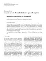
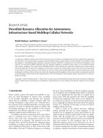
Figure 1: The road map of the simulation scenario. Although the
figure presents a constant velocity ABCD path and a 90
◦
road-
departure angle, for the comparison in Section 5,theonroadveloc-
ity is perturbed with random accelerations and the departure angle
varies randomly between 20–160
◦
.
(Figure 1) in which a vehicle moves on and off the road. The
vehicle moves with a nominal constant velocity, perturbed
by a random Gaussian noise, and its dynamics evolve in the
tracking state space according to the following equation:
x
k
= Fx
k−1
+ Gu
k−1
. (1)
The state vector x
k
= [x
k
y
k
˙
x
k
˙

y
k
]
T
consists of the vehicle’s
position and velocity and the noise vector u
k
= [u
x
k
u
y
k
]
T
of
random accelerations, both based on the Cartesian x-y plane.
We assume Gaussian system noise u
k
∼N (0, Q
k
), with Q
k
its
diagonal 2
×2 covariance matrix. The state transition matrix
F and the state noise matrix G are
F
=
⎡

⎢
⎢
⎢
⎣
10T 0
010T
001 0
000 1
⎤
⎥
⎥
⎥
⎦
, G =
⎡
⎢
⎢
⎢
⎣
T
2
/20
0 T
2
/2
T 0
0 T
⎤
⎥
⎥

⎥
⎦
,(2)
where T is the measurement update rate.
The radar lies at the origin of the plane at point (x, y)
=
(0, 0) and feeds the tracking algorithm with noisy measure-
ments of the azimuth angle and range of the vehicle. The
measurement equation is given next:
z
k
= h

x
k

+ v
k
. (3)
The measurement vector z
k
= [θ
k
r
k
]
T
consists of the vehicle
azimuth angle and range in the polar plane. The nonlinear
function h(

·) that maps the state—with the measurement—
space is
h

x
k

=

arctan(y
k
/x
k
)

x
2
k
+ y
2
k

,(4)
G. Kravaritis and B. Mulgrew 3
where the top element accounts for the azimuth angle of the
vehicle and the bottom for its range, given its Cartesian posi-
tion (x
k
, y
k

). The measurement noise vector v
k
= [v
θ
k
v
R
k
]
T
models the radar’s azimuth and range inaccuracy, where
v
k
∼N (0, R
k
)inwhichR
k
is the diagonal 2 ×2 noise covari-
ance matrix.
Generally in vehicle tracking we assume that some fea-
tures on the ground scene of interest force locally the vehicle
to move under specific patterns. Some of the features (like
bridges and lakes [27]) impose hard constraints on the ve-
hicle movement, whereas other (roads in our study) impose
soft constraints. The objective in this class of problems is to
incorporate efficiently a-priori knowledge of these features
into the tracking algorithm.
In this work we assume that a vehicle travels on a terrain
with known road structure, having the ability to move on
and off the road. The roads impose probabilistic constraints

on the movement of the vehicle which implies that when the
vehicle is on the road the uncertainty for its state is larger
along the road than orthogonal to it. We model this by set-
ting the variance of the process noise along the road, σ
{u
α
k
}
2
,
larger than the variance orthogonal to it σ
{u
o
k
}
2
. The direc-
tion of the on-road noise depends on the direction of the
road. Therefore the associated process noise covariance Q
k
is
rotated using the following relation:
Q
on,k
(ψ) = Ω
ψ

σ

u

o
k

2
0
0 σ

u
α
k

2

Ω
T
ψ
,(5)
where Ω
ψ
is the rotational transformation matrix and ψ is
the angle of the road measured clockwise from the y-axis:
Ω
ψ
=

−
cos ψ sin ψ
sin ψ cos ψ

. (6)

For off-road motion since the vehicle travels unconstrained,
we use the same process noise variances for both x-andy-
axes, σ
{u
x
k
}
2
= σ{u
y
k
}
2
; the covariance thus becomes
Q
off,k
=
⎡
⎣
σ

u
x
k

2
0
0 σ

u

y
k

2
⎤
⎦
. (7)
For notational purposes we define R
s
as the set of the
roads r on the ground scene of interest. For off-road motion
we use the convention r
= 0. Consider that both VSMMPF
and VMPF vehicle trackers employ nominally N
f
particles
{x
i
k
}
N
f
i=1
. In contrast to the VSMMPF which always uses N
f
particles, the VMPF uses a varying number of particles which
is smaller or equal to N
f
. In both algorithms each particle is
associated with a mode M

i
k
according to the following:
M
i
k
=

r if particle x
i
k
is on the road r,wherer ∈ R
s
,
0ifparticlex
i
k
is off-road.
(8)
For instance, if in the simulation scenario the vehicle can
move freely among three roads (R
s
={1, 2, 3}) and can also
travel off-road, each particle x
i
k
will be assigned with one of
the possible modes: M
i
k

= 1, 2, 3, or 0. For further analysis
and examples of this modal approach and a description of
the VSMMPF algorithm, please refer to [12, 17]. Next we
introduce and discuss the variable-mass particle allocation
principle.
3. VARIABLE-MASS TECHNIQUE
This section introduces the variable-mass mechanism and
discusses its strengths and benefits.
3.1. The proposed approach
In this part we first summarise the VSMMPF logic for al-
locating the particles to the multiple modes and then in-
troduce the VMPF approach. Consider an n
m
-mode parti-
clefilterwhichattimek
− 1hasN
α,k−1
particles at mode α.
At k each particle can either continue on the same mode or
switch to another. Let the known a priori probability switch-
ing
1
from mode α to mode β be p
α→β
∈ R[0, 1],
2
where
α, β
∈ N[1, n
m

]; R and N are, respectively, the sets of the real
and natural numbers. According to the VSMMPF, the num-
ber of the transferred particles to a mode is proportional to
the fixed prior mode probability:
N
α→β,k
=




ν
i
<p
α→β
:

ν
i
: ν
i
∼U(0, 1)

N
a,k−1
i=1





,(9)
where N
α→β,k
is the number of the particles that are trans-
ferred from mode α to mode β at k and U(
·, ·) stands for
the uniform distribution. For a large number of particles, we
have
lim
N
α,k−1
→∞
N
α→β,k
|
N
α,k−1
= p
α→β
·N
α,k−1
, (10)
which indicates that on average we get
N
α→β,k
= p
α→β
·N
α,k−1
. (11)

Furthermore, for the VSMMPF it holds that
n
m

β=1
N
α→β,k
= N
α,k−1
, ∀α, (12)
which implies that the overall number of its particles remains
constant.
Consider again the n
m
-mode particle filter defined previ-
ously. In the VMPF, we can change the number of the parti-
cles according to an arbitrary defined probabilistic parame-
ter, γ
α→β,k
∈ R[0, 1], which we call gamma metric:
N

α→β,k
= γ
α→β,k
·N
α,k−1
, (13)
1
A switch from mode α to β refers to a change of the particle propagation

model from the one of mode α to β.
2
The case β = α refers to continuation on the same mode.
4 EURASIP Journal on Advances in Signal Processing
where N

α→β,k
is the transferred number of particles from
mode α to β at k.Forγ
α→β,k
,itholds
n
m

β=1
γ
α→β,k
= 1, ∀α, k. (14)
We d efi ne m
α→β,k
as the mass of the particles that are trans-
ferred from mode α to β at k:
m
α→β,k
=
p
α→β
γ
α→β,k
= p

α→β
·
N
α,k−1
N

α→β,k
. (15)
The masses are used to rescale the weights of the particles, so
as the arbitrary particle allocation not to bias the final esti-
mates (if the weights were left unscaled, then the state esti-
mate would be biased towards the modes which the gamma
metric “favoured”).
In contrast to the VSMMPF, see (12), the total number of
the VMPF particles is allowed to vary:
n
m

β=1
N

α→β,k
=N
α,k−1
, ∀α. (16)
A stepwise algorithm for the variable-mass technique for a
general multimodel particle filter is given in the appendix.
3.2. Justification
Equation (13) is the key to the proposed particle alloca-
tion scheme, which (a) enables the particles to be allocated

to their modes more deterministically than within the VS-
MMPF, and (b) allows the proportion of the allocated parti-
cles to vary with time k. With this features the algorithm can
precisely and freely allocate the number of its particles to the
different modes at each k. The assignment of the particles
with appropriate masses keeps the estimates unbiased from
the arbitrary particle allocation.
Essentially, the variable-mass mechanism introduces an-
other degree of freedom to the estimation process, by em-
ploying particle triples consisting of
{state, weight, mass}.
The extra degree of freedom, the mass, enables the estima-
tortoexploitindirectly additional information, which is ex-
pected to increase the efficiency of the particles, affecting
both the estimation accuracy and the computational load
of the tracker. This additional information might concern,
for instance, the estimation difficulty of particular subspaces
of the estimation space. The algorithm, thus, can use fewer
particles in a mode which has relatively simple and linear
state prediction dynamics. In contrast it can use more par-
ticles when the mode dynamics are more difficult due to
intense model nonlinearities and/or multimodalities of the
posterior-state probability density function (pdf). The extra
information can also concern directly the measurements. For
instance, if a measurement indicates that a mode is highly
unlikely (i.e., its particles will be most probably assigned with
negligible weights), the algorithm can allocate fewer particles
to it and more to the more likely modes, so as totally the par-
ticles to be assigned with bigger weights and thus contribute
more to the state estimation process.

Overall, the proposed approach can be described as an
eclectic spatial enhancement or degradation of the resolu-
tion of the discrete approximation of the posterior-state pdf,
p(x
k
, z
k
). This manipulation of the resolution, or else of the
particles’ density, is allowed since the variable masses rescale
appropriately the particles’ weights for debiasing the final es-
timate. It is characterised as “spatial” since it alters the par-
ticle density only on specific areas, in contrast to “universal”
which would imply simply the change of the total number of
particles N
f
.
4. VARIABLE-MASS PARTICLE FILTER
We begin this section by outlining the features of the vehicle-
tracking VMPF and then we describe in detail how the spe-
cific algorithm works.
4.1. Features of the vehicle tracker
The VMPF employs the varying mass technique for propa-
gating its on-road particles on and off the road. Specifically
for these particles, the tracker uses as the gamma metric an
approximation of the posterior-mode probabilities, obtained
by fusing the fixed prior mode probabilities with the varying
modes’ likelihoods conditioned on the current measurement.
As described before, the varying masses that the algorithm
uses, compensate for the resulting over- or under-population
of its modes. The fact that in contrast to the VSMMPF, the

VMPF is not “blind” to the measurements when allocating
its on-road particles to their corresponding modes results in
amoreefficient particle use, which translates consequently to
a performance improvement. For the off-road particles, both
algorithms use a similar propagation mechanisms.
Another feature of the new vehicle tracker is that it em-
ploys just one particle on the road. This is because the on-
road dynamics are easier to estimate due to the soft con-
straints that the roads themselves impose [28]. Following the
varying-mass logic, the mass of that on-road particle is pro-
portional to the posterior probability of the on-road mode.
Compared to the VSMMP, the fact that the variable mass
approach allows the tracker to use just one particle for this
mode, results in significant computational gains when the
vehicle travels on the road.
For the prediction of the on-road particle the VMPF em-
ploys a Kalman filter. For running the KF, it converts the 2D
polar radar measurements to 1D Cartesian pseudomeasure-
ments (approximated as Gaussian) that lie in the middle of
the road. The KF operates in a reduced-dimension 2D state-
space along the middle of the road and feeds the tracker with
estimates of the mean and covariance of the on-road states.
These estimates are transformed and placed into the original
4D tracking state-space to finally form the on-road particle.
The estimated on-road probability distribution from the KF
is used also in the prediction step, to draw particles randomly
and propagate them off the road. The number of these de-
parting particles is determined from the posterior road-exit
mode probabilities.
G. Kravaritis and B. Mulgrew 5

x-axis
y-axis
Road
Measurement
Pseudomeasurement
AB
C1 C2
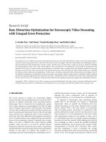
Figure 2: The skewed ellipse (dashed line) around the measure-
ment z
c
k
is a vertical section of the measurement pdf. The pseu-
domeasurement,
z
on,k
, is set on the mode of the distribution result-
ing from the cross-section of line AB (the middle of the road) with
the measurement pdf and is fit with a one-dimensional Gaussian
pdf (dot-dashed line, rotated 90
◦
for illustration).
4.2. The algorithm
For the sake of clarity, we do not consider a junction or bridge
prediction model as in [12] and focus just on an environment
with a vehicle travelling on and off nonintersecting roads.
The VMPF consists of a prediction, an update, and a resam-
pling step, which we describe next.
4.2.1. Prediction step
In the prediction step, the algorithm predicts the particles
one step ahead according to their mode dynamics. First we

describe the prediction phase for the road particles and then
for the off-road particles.
Prediction of the on-road particles
This phase consist of the prediction of the on-road particles
which either continue on the road or depart from it. We em-
ploy one particle for modelling the on-road motion. For the
on-road prediction, we first generate an on-road pseudomea-
surement
z
on,k
with its associated variance and then apply a
KF. We consider Figure 2 assuming that line AB lies in the
middle of the road. For clarity and simplicity in our analysis,
the roads are set parallel to the x-axis.
At time instant k, we receive a radar measurement z
k
=
[θ
k
r
k
]
T
which we transform to the Cartesian plane to obtain
z
c
k
:
z
c

k
= h
−1

z
k

=

r
k
·cos θ
k
r
k
·sin θ
k

. (17)
Theskewedellipsearoundz
c
k
at Figure 2, is the n
σ
th stan-
dard deviation (
σ
z,k
) confidence interval of the measurement
noise, after being transformed to the Cartesian plane us-

ing function h
−1
(·)from(17). C1 = (x
C1
, y
C1
)andC2 =
(x
C2
, y
C2
) are the cross-section points of the interval and the
middle of the road. The value of n
σ
is chosen arbitrary (usu-
ally 3-4) since later (18) cancels it out.
The assumption here is that the cross section of line AB
and the 2D skewed-Gaussian measurement noise pdf can
be approximated as a 1D Gaussian pdf along AB. There-
fore, since we are also using a linear constant velocity vehicle
model, we track on-road on a reduced state-space (along AB)
with a 2D Kalman filter. The tracking space of the KF consists
of the vehicle’s position x
on,k
and velocity
˙
x
on,k
just along the
middle of the road. This is because an attempt to track any

possible on-road movement orthogonal to the road will have
negligible significance; especially since the roads seem to have
zero width when the radar is far.
For computing the pseudomeasurement
z
on,k
on AB we
find the point within the segment C1C2 which maximises
the measurement likelihood (i.e., the statistical mode)andfit
to it a Gaussian pdf. The standard deviation of the pdf can be
approximated numerically as
σ
z,on,k
=


x
C1
−x
C2


n
σ
. (18)
Using
z
on,k
, we predict the on-road particle x
2D

on,k
−1
one
step ahead with the following set of KF equations:
x
2D−
on,k
= F
on
·x
2D
on,k
−1
,
P
−
on,k
= F
on
·P
on,k−1
·F
T
on
+ G
on
·Q
on
·G
T

on
,
K
k
= P
−
on,k
·H
on
·

H
on
·P
−
on,k
·H
T
on
+

R
on,k

−1
,
x
2D
on,k
= x

2D−
on,k
+ K
k
·

z
on,k
−H
on
·x
2D−
on,k

,
P
on,k
=

I −K
k
·H
on

·P
−
on,k
,
(19)
where

F
on
=

1 T
01

, G
on
=

T
2
/2
T

, Q
on
= σ
2
α
, H
on
= [0 1].
(20)

R
on,k
=(σ
z,on,k

)
2
is the variance of z
on,k
and x
2D
on,k
=[x
on,k
˙
x
on,k
]
T
is the truncated 2D version of the on-road particle. We aug-
ment then the x
2D
on,k
and place it into the original 4D state-
space:
x

on,k
=
⎡
⎢
⎢
⎢
⎣
x

on,k
y
on,k
˙
x
on,k
0
⎤
⎥
⎥
⎥
⎦
, (21)
where y
on,k
is the y-axis value of the middle of the road.
Next we compute the likelihood of the vehicle continu-
ing on the road or departing from it. For that, we employ
6 EURASIP Journal on Advances in Signal Processing
n
φ
road prediction submodes
3
M
j
φ,k
, for the following set of
propagation angles:

φ

j

n
φ
j=1
=

φ
1
, , φ
n
φ

, (22)
where φ
j
is the departure angle of the particles of the jth sub-
mode, measured anti-clockwise from the road. As a conven-
tion, we always set φ
1
= 0
◦
accounting for the on-road prop-
agation. The nominal positions x
j−
φ,k
of the road-prediction
submodes M
j
φ,k

are given by the following relation:
x
j−
φ,k
=
⎡
⎢
⎢
⎢
⎣
x
on,k−1
+

x
on,k
−x
on,k−1

·cos φ
j
y
on,k−1
+

x
on,k
−x
on,k−1


·sin φ
j
˙
x
on,k−1
·cos φ
j
˙
x
on,k−1
sinφ
j
⎤
⎥
⎥
⎥
⎦
, (23)
where j
∈{1 n
φ
}. According to (23), the x
j−
φ,k
are cal-
culated by propagating from k
− 1tok the position of the
on-road particle and rotating it according to the correspond-
ing angle φ
j

. The probability of each submode is then com-
puted by transforming each x
j−
φ,k
to the measurement space
and computing its likelihood according to the measurement
z
k
and its covariance R
k
:

p
j
φ,k
= p

M
j
φ,k
| z
k

=
N

h

x
j−

φ,k

, R
k

, (24)
where h(
·)isdefinedin(4). The normalised probabilities are
p
j
φ,k
=

p
j
φ,k

n
φ
ζ=1

p
ζ
φ,k
. (25)
We then use a weighted sum of the varying p
j
φ,k
and the
fixed prior probability

p:

p
j
k
=
⎧
⎪
⎪
⎨
⎪
⎪
⎩
w
p
·p +

1 −w
p

·
p
j
φ,k
, j = 1 (on-road),
w
p
·

1 − p


(n
φ
−1)
+

1 −w
p

·
p
j
φ,k
, j=1 (on-road),
(26)
3
If a particle which at k − 1 is lying on the road, r (i.e., M
i
k
−1
= r)is
to be propagated with the VSMMPF, there are two possibilities: either
to continue on the same road (M
i
k
= M
i
k
−1
= r)ortodepartfromit

(M
i
k
= 0). For the latter case, the VSMMPF just uses the mode-transition
probability p
r→0
. The particular version of the VMPF that we study here
accounts for n
φ
− 1 (since φ
1
= 0
◦
)different road exit angles. Thus, in
contrast to the VSMMPF, rather than using one mode-transition prob-
ability for road departure, the p
r→0
, the VMPF employs n
φ
− 1, the
p
r→M
2
φ,k
, p
r→M
3
φ,k
, , p
r→M

n
φ
φ,k
, or for convenience {p
j
k
}
n
φ
j=2
.Thisiswhywe
prefer to use the term submode for the M
j
φ,k
—since all the {p
j
k
}
n
φ
j=2
are
subcases of p
r→0
. Regarding the case that the particle stays on the road,
the probability p
1
k
is equivalent to p
r→r

. Therefore, note that there is not
any qualitative difference between the terms “mode” and “submode” in
this article, and the specific terminology is used just for the sake of con-
sistency.
where 0 ≤ w
p
≤ 1 is a user defined parameter. A value of w
p
closer to 1 weights more the prior p whereas closer to 0 more
the measurement-dependent p
j
φ,k
. The final normalised sub-
mode probability is given by
p
j
k
=

p
j
k

n
φ
ζ=1

p
ζ
k

. (27)
We us e p
j
k
as the gamma metric from (13)tocalculate
the number of the particles N
j
φ,k
that we will allocate to each
submode M
j
φ,k
:
N
j
φ,k
= p
j
k
·N
on,k−1
, (28)
where N
on,k−1
is the nominal number of the on-road particles
at k
−1 (as we will see later the resampling step spawns tem-
porally N
on,k
on-road particles, which are later discarded).

As described before, for the on-road submode ( j
= 1), ir-
respectively of (28), we are always employing one particle
(N
j
φ,k
|
j=1
= 1). Next, according to p
j
k
, we predict a number of
particles off the road. First, we generate the particles required
by sampling the on-road state pdf (P
on,k−1
), derived from the
KF at the previous time instant:

x
i
off,k

N
o
off,k
i=1
=


x

i
off,k
˙
x
i
off,k

T

N
o
off,k
i=1
∼N

x
on,k−1
, P
on,k−1

,
(29)
where N
o
off,k
=

n
φ
j=2

N
j
φ,k
The new-born particles {x
i
off,k
}
N
o
off,k
i=1
which initially lie on the road are propagated off the road
according to the mode departure angles
{φ
j
}
n
φ
j=1
, using the
relation below:
x
ij
off,k
=
⎡
⎢
⎢
⎢
⎢

⎢
⎢
⎢
⎢
⎢
⎢
⎢
⎢
⎣
x
i
off,k
·tan φ
j
−x
on,k−1
·tan

φ
j
/2

tan φ
j
−tan

φ
j
/2


tan φ
j
·

x
i
off,k
·tan φ
j
−x
on,k−1
·tan

φ
j
/2


tan φ
j
−tan

φ
j
/2

−
x
i
off,k

·tan φ
j
+ y
on,k−1
˙
x
i
off,k
·cos φ
j
˙
x
i
off,k
·sin φ
j
⎤
⎥
⎥
⎥
⎥
⎥
⎥
⎥
⎥
⎥
⎥
⎥
⎥
⎦

.
(30)
Finally, we partition the resulting particles to the ones that
lie right (clockwise),
{x
ζ,R
off,k
}
N
R
off,k
ζ=1
, and left (anti-clockwise),
{x
ζ,L
off,k
}
N
L
off,k
ζ=1
, from the road. For them it holds


x
ζ,R
off,k

N
R

off,k
ζ=1
,

x
ζ,L
off,k

N
L
off,k
ζ=1

=


x
ij
off,k

N
j
φ,k
i=1

n
φ
j=2
, (31)
where N

R
off,k
+ N
L
off,k
= N
o
off,k
.
Prediction of the off-road particles
We continue with the second phase and we predict the parti-
cles which were off-road at k
−1(i.e.,M
i
k
−1
= 0) following the
G. Kravaritis and B. Mulgrew 7
off-road prediction scheme of the VSMMPF. Consider that
we have N
off,k
such particles. We preliminary propagate every
particle with equation
x
i−
off,k
= Fx
i
k
−1

. (32)
We introduce then the following binary function:
c

x
i
k
−1
, r

=

1ifx
i
k
−1
−→ x
i−
off,k
crosses road r=0,
0 otherwise.
(33)
The mode transition probabilities (p
M
i
k
−1
→M
i
k

)aregivenby
p
0→r

x
i
k
−1

=
⎧
⎪
⎪
⎪
⎪
⎪
⎪
⎨
⎪
⎪
⎪
⎪
⎪
⎪
⎩
p

if c

x

i
k
−1
, r

=
1,
0ifc

x
i
k
−1
, r

=
0,
d

x
i−
off,k
, r

>τ,
p


τ −d


x
i−
off,k
, r

τ
otherwise,
(34)
where p

is the user-defined probability that the vehicle en-
ters a road when crossing, d(x
i−
off,k
, r) is the shortest distance
from particle x
i−
off,k
to the road r,andτ is a user defined
threshold according to the acceleration capabilities of the ve-
hicle. The probability that the particle will remain off-road
is
p
0→0

x
i
k
−1


=
1 − p
0→r

x
i
k
−1

. (35)
The mode M
i
k
is randomly drawn according to the asso-
ciated transition probabilities:
P

M
i
k
= r

= p
M
i
k
−1
→r



r∈{0,R
s
}
. (36)
If M
i
k
= 0, the mode implies that the particle stays off
the road and therefore we propagate it simply by using the
state transition equation with a random noise sample u
i
k
−1
:
x
i
off,k
= Fx
i
k
−1
+ Gu
i
k
−1
. (37)
If M
i
k
=0, the particle is positioned at the shortest point on

the road and its velocity is rotated, using the rotation ma-
trix (6), randomly towards one road direction. All predicted
particles from this phase are denoted as
{x
i
off,k
}
N
off,k
i=1
.
The resulting set of the particles from the prediction step
finally becomes

x
i
k

N
v,k
i=1
=

x

on,k
,

x
ζ,R

off,k

N
R
off,k
ζ=1
,

x
ζ,L
off,k

N
L
off,k
ζ=1
,

x
ζ
off,k

N
off,k
ζ=1

,
(38)
where N
v,k

stands for the total number of particles that the
VMPF uses at the specific time instant k:
N
v,k
= 1+N
off+,k
+ N
off,k
. (39)
4.2.2. Update step
At the beginning of the update step we weight each particle
in the VSMMPF fashion:
w
i
k
= p

z
k
| x
i
k

=
N

h

x
i

k

, R
k

, (40)
and we normalise its weight:
w
i
k
=

w
i
k

N
v,k
j=1
w
j
k
, (41)
where in analogy with (31)weobtain

w
i
k

N

v,k
i=1
=

w
on,k
,

w
ζ,R
off,k

N
R
off,k
ζ=1
,

w
ζ,L
off,k

N
L
off,k
ζ=1
,

w
ζ

off,k

N
off,k
ζ=1

.
(42)
At this point we calculate the particles’ masses. Just for
illustration, we present once more the relation (15)whichwe
use to compute the masses:
m
α→β,k
= p
α→β
·
N
α,k−1
N

α→β,k
. (43)
The particles obtain a mass according to the subset in which
they belong. The mass of the on-road particle is
m
on,k
= p·
N
on,k−1
1

, (44)
since at k
− 1 we nominally had N
on,k−1
particles on road, p
was the probability for the particles to remain on-road and
the current mode uses one particle.
The masses of the particles that were predicted departing
from the road are
m
R
off,k
=
1 − p
2
·
N
on,k−1
N
R
off,k
,
m
L
off,k
=
1 − p
2
·
N

on,k−1
N
L
off,k
.
(45)
Using the same logic as before, we had previously N
on,k−1
par-
ticles on the road, (1
− p)/2 was the probability for the par-
ticles to exit either right of left the road and N
R
off,k
and N
L
off,k
was their respective number.
For the particles that were off-road at k
− 1, using a
varying-mass analogy, we argue that their prediction was
within a single mode and consequently are set with unitary
masses:
m
off,k
= 1·
N
off,k−1
N
off,k

= 1. (46)
We derive then the scaled weights of the particles by mul-
tiply them with their corresponding masses:
w

on,k
= m
on,k
·w
on,k
,


w
i,R
off,k

N
R
off,k
i=1
= m
R
off,k
·

w
i,R
off,k


N
R
off,k
i=1
,


w
i,L
off,k

N
L
off,k
i=1
= m
L
off,k
·

w
i,L
off,k

N
L
off,k
i=1
,



w
i
off,k

N
off,k
i=1
= m
off,k
·

w
i
off,k

N
off,k
i=1
,
(47)
8 EURASIP Journal on Advances in Signal Processing
which are subsequently normalised to sum to 1:
w
i
k
=

w
i

k

N
v,k
j=1
w
j
k
, (48)
where


w
i
k

N
v,k
i=1
=


w

on,k
,


w
ζ,R

off,k

N
R
off,k
ζ=1
,


w
ζ,L
off,k

N
L
off,k
ζ=1
,


w
ζ
off,k

N
off,k
ζ=1

.
(49)

The state estimate at k is finally given by the weighted
sum of the particles:
x
k
=
N
v,k

i=1
w
i
k
x
i
k
. (50)
4.2.3. Resampling step
The next step is to resample the weighted particle set to dis-
card particles with small weights. The order of the parti-
cles and their weights should remain unaltered as in (31)
and (42). We use the systematic resampling algorithm (see
Algorithm 1), modified accordingly for the VMPF (see above
for the pseudo-code). Its characteristic now is that it treats
the on-road particle as the parent of multiple particles with
the same states, with multiplicity proportional to the on-road
mass m
on,k
. For this reason, we use the unscaled versions of
the weights as computed in (41). After resampling, the size of
the resulted resampled particle set

{x
i
k
}
N
f
i=1
is increased from
N
v,k
to N
f
and all particles obtain equal weights and masses.
The final step of VMPF is to re-estimate the states of the
on-road particle, accounting for particles that might have en-
tered the road. Let us assume that after resampling N
on,k
par-
ticles lie on the road
{x
i,r
on,k
}
N
on,k
i=1
. Since these post-resampling
particles have equal weights, the characterisation of the on-
road posterior pdf is given just by their density. For comput-
ing the final posterior on-road particle, x

on,k
, under the as-
sumption of Gaussianity, we simply calculate the mean state
of
{x
i,r
on,k
}
N
on,k
i=1
:
x
on,k
=
1
N
on,k
·
N
on,k

i=1
x
i,r
on,k
. (51)
Only the x
on,k
is forwarded to the next time step k +1while

the set
{x
i,r
on,k
}
N
on,k
i=1
is discarded.
5. SIMULATION RESULTS
In this section we study the performance of the tracking al-
gorithms using the road structure of Figure 1. For a fair com-
parison we use the same parameters as in [12, 22]. The vehi-
cleismovingalongpointsA,B,CandD.Itmoveson-road
along segments AB and CD and off-road along BC. In the
Monte Carlo (MC) runs that we perform, we vary the angle
of departure ϕ randomly uniformly between 20
◦
<ϕ<160
◦
.
Set nominal number of on-road particles:
N
res
on,k
= N
f
−N
v,k
+1

Initialise the cumulative density function
(cdf) of the weights: c
1=w
1
k
for i = 2:N
res
on,k
do
Construct cdf: c
i
= c
i−1
+ c
1
end for
for i
= (N
res
on,k
+1):N
f
do
Construct cdf: c
i
= c
i−1
+ w
(i−N
res

on,k
+1)
k
end for
Start at the bottom of the cdf: i
= 1
Draw a starting point: u
1
∼U(0, c
N
f
/N
f
)
for j
= 1:N
f
do
Move along the cdf:
u
j
= u
1
+(c
N
f
/N
f
)·(j −1)
while u

j
>c
j
do
i
= i +1
end while
if i<N
res
on,k
+1then
Assign sample: x
j
k
= x
i
k
else
Assign sample: x
j
k
= x
(i−N
res
on,k
+1)
k
end if
end for
Algorithm 1: VMPF resampling.

The total simulation steps are 60 (20 for each segment) and
the radar update rate is T
= 5 seconds. The width of the road
is 8 m.
The nominal velocity of the vehicle is 12 m/s which on-
road is perturbed along its direction by random accelerations
with standard deviation σ
a
= 0.6m/s
2
. The radar has angular
accuracy 0.5
◦
and range resolution 20 m. The standard devia-
tion of the process noise is σ
x
= σ
y
= 0.6m/s
2
(off-road) and
σ
o
= 0.0001 m/s
2
(orthogonal to the road). We set the mode
probabilities
p = p
∗
= 0.98 and the threshold τ = 18.75 For

the VMPF we set w
p
= 0.5, in (26), weighting thus equally
the prior and the measurement-dependent mode probabili-
ties. A smaller w
p
value would improve the transition from
on- to off-road and worsen the on-road performance; for a
larger value the opposite would hold.
We use a VSMMPF, one VMPF with n
φ
= 3(whichwe
call VMPF
3φ
) and one VMPF with n
φ
= 7:
{φ
j
}
3
j
=1
={0
◦
,90
◦
, 270
◦
},


φ
j

7
j
=1
=

0
◦
,45
◦
,90
◦
, 125
◦
, 225
◦
, 270
◦
, 315
◦

.
(52)
The performance gains of the VMPF
3φ
come solely from its
varying-mass structure, whereas from the VMPF come as

well from the more departure angles it considers. For our
analysis we vary the nominal number of the particles of the
trackers: N
f
= 10, 25, 50, 75, 100, 250, 500, 1000. For ev-
ery N
f
we perform 3000 MC runs and we measure the on-
and off-road root mean square (RMS) position error, the
maximum value of the position error overshoot when the
vehicle departs from the road, the number of the particles
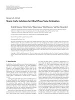
G. Kravaritis and B. Mulgrew 9
6420−2−4−6−8−10−12
×10
2
x (m)
1800
2000
2200
2400
2600
2800
3000
3200
y (m)
Roads
Vehicle path
VMPF
VMPF
3φ

VSMMPF
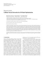
Figure 3: The true vehicle track and the estimates of the trackers for
a representative example in which the road-departure angle is 128
◦
and N
f
= 50.
that VMPF uses, and the on-road CPU time. All algorithms
were initialised by randomly seeding particles about the true
states.
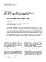
Figures 3 and 4 present, respectively, the vehicle tracks
and the RMS position error of the three trackers, in a rep-
resentative example in which N
f
= 50 and ϕ= 128
◦
. For the
particular run, when the vehicle was on the road, both VMPF
and VMPF
3φ
employed about half of the particles that the
VSMMPF used. From the figures we observe that although
all algorithms attained a similar performance on-road, when
the vehicle departed from the road, the transient response of
the VSMMPF was considerably slower and less accurate.
Figure 5 shows the on-road RMS position error of the fil-
ters over the nominal number of the particles N
f
after the
MC analysis. The VMPF demonstrates better performance

than the VSMMPF for N
f
< 138, while for bigger values it
converges to a slightly sub-optimal (1.1% for N
f
= 1000)
RMSE. Compared to the VMPF
3φ
, the VMPF has smaller
RMSE for N
f
< 90 because it uses more road-exit submodes
and thus more particles. For N
f
> 90, the on-road VMPF
3φ
performance is better, because the fact that it considers just
±90
◦
road-exit turns, as N
f
increases, makes it more ro-
bust to measurement noise. The VMPF
3φ
improvement of
the performance over the VSMMPF for N
f
> 83 is due to the
on-road Kalman filtering propagation mechanism.
From Figures 6 and 7 we witness that the off-road tran-

sient response of the VMPF during road segment BC is over-
all superior. We remind here that when the vehicle is off-road,
the estimation schemes for both VMPF and VSMMPF con-
verge to the same unconstrained sequential importance re-
sampling particle filter. The difference in performance that
we observe is the result of the different mechanisms for prop-
agating off the road the on-road vehicle. From Figure 7 we
see that even when N
f
= 1000, the VMPF has 36% smaller
6050403020100
k
0
20
40
60
80
100
120
Position error (m)
VMPF
VMPF
3φ
VSMMPF
Figure 4: Comparison of the position error of the algorithms for
the above example. The horizontal dotted lines indicate the off-road
interval.
10
3
10

2
10
1
N
f
10
20
30
40
50
60
70
80
90
Position RMSE on-road (m)
VMPF
VMPF
3φ
VSMMPF
Figure 5: Comparison of the RMS position error when the vehicle
is on-road, over the nominal number of particles N
f
.
overshoot than the VSMMPF. Once more, the VMPF
3φ
per-
formance shows us which amount of performance improve-
ment comes just from the varying-mass particles technique.
Figure 8 shows the percentage of the particles that the
VMPF and VMPF

3φ
use over the nominal number of parti-
cles N
f
. When the vehicle is on-road, the algorithms use, re-
spectively, about 33%–41% and 19%–29% of the N
f
. When
the vehicle exits the road, they rapidly increase their num-
ber of particles until reaching N
f
. For continuing our anal-
ysis, we define as the particle efficiency f of VMPF over
10 EURASIP Journal on Advances in Signal Processing
Table 1: Particle efficiency: the ratio of the number of the VSMMPF particles to the VMPF particles for a given performance. We focus on
the RMS position error, when the vehicle is on-road and off-road, and on the RMS transient overshoot, when the vehicle departs from the
road.
RMSE on-road
RMSE (m) 19.58 23.43 27.29 31.14
VSMMPF number of particles-N
f
339.77 70.62 49.62 41.46
VMPF average number of particles 337.51 8.62 5.26 4.10
Particle efficiency f 1.01 8.19 9.43 10.11
RMSE on-road
RMSE (m) 35.55 51.66 67.77 83.88
VSMMPF number of particles-N
f
1000.00 188.19 91.18 63.62
VMPF average number of particles 240.93 33.72 16.26 9.54

Particle efficiency f 4.15 5.58 5.61 6.67
RMSE transient overshoot
RMSE (m) 54.20 67.61 81.01 94.42
VSMMPF number of particles-N
f
1000.00 369.23 201.82 130.30
VMPF average number of particles 72.64 25.13 14.86 9.54
Particle efficiency f 13.77 14.69 13.58 13.66
10
3
10
2
10
1
N
f
20
40
60
80
100
120
140
160
180
200
Position RMSE off-road (m)
VMPF
VMPF
3φ

VSMMPF
Figure 6: Comparison of the RMS position error when the vehicle
is off-road, over the nominal number of particles N
f
.
VSMMPF as the ratio of the number of the VSMMPF part icles
to the VMPF particles for a given performance.Forexample
f (20)
= 2 for on-road RMSE indicates that the VSMMPF
employs 2 times more particles than the VMPF, when both
attain a 20 m on-road RMSE. Using Figures 5, 6, 7,and8,we
calculate f for the various performance metrics. The results
are presented at Tabl e 1 and demonstrate the efficiency of the
proposed algorithm. In the studied scenario, the VSMMPF
uses up to 14.69 times more particles than the VMPF for
achieving the same performance, in the RMSE ranges within
which f could be calculated.
Finally, Figure 9 compares the on-road CPU time of the
algorithms(runonaLinuxplatformwithanIntelXeon
10
3
10
2
10
1
N
f
0
50
100

150
200
250
Position RMSE transient overshoot (m)
VMPF
VMPF
3φ
VSMMPF
Figure 7: Comparison of the RMS position error overshoot when
the vehicle departs from the road, over the nominal number of par-
ticles N
f
.
3 GHz processor and a 1 GB DDR2 memory). For N
f
< 40,
the VMPF trades off its on-road performance superiority
compared to the VSMMPF with computing power. For larger
values of N
f
, the VMPF is computationally cheaper and has a
CPU time linearly related to the N
f
. On the road, depending
on the N
f
,VMPF
3φ
requires 6%–23% less CPU time than
the VMPF, while using on average almost half of the particles

(Figure 8). Off the road all algorithms had the same com-
putational demands. On the robustness of the algorithms,
we observe poor performance of the VSMMPF for N
f
= 10
and 25, where it resulted, respectively, in 40.5% and 9.1% di-
verged runs (resp., 8.1 and 3.7 times more than the VMPF).
Nevertheless, for bigger—and more realistic—values of N
f
,
G. Kravaritis and B. Mulgrew 11
10
3
10
2
10
1
N
f
10
20
30
40
50
60
70
80
90
100
Percentage of VMPF particles (%)

On-road VMPF
Off-road VMPF
On-road VMPF
3φ
Off-road VMPF
3φ
Figure 8: The percentage of the particles of the VMPF and VMPF
3φ
to the particles of the VSMMPF (when the vehicle is on- and off-
road), over the nominal number of particles N
f
.
10
3
10
2
10
1
N
f
0
0.01
0.02
0.03
0.04
0.05
0.06
0.07
0.08
0.09

On-road CPU time (s)
VMPF
VMPF
3φ
VSMMPF
Figure 9: Comparison of the CPU time when the vehicle is on-road,
over the nominal number of particles N
f
.
both algorithm did demonstrate a robust performance. An
algorithm was considered to be diverged if at any point its
position error exceeded 600 m. All the simulation results pre-
sented in this section were calculated just from the converged
runs.
6. CONCLUSIONS
This work introduced the variable-mass particle filter and
used the terrain-aided tracking problem for comparing it
with the variable-structure multimodel particle filter. Both
Compute, where defined, the gamma metric:
for α
= 1:n
m
for β = 1:n
m
if α→β is defined
Compute: γ
α→β,k
end
end
end

Calculate the number of the particles of each
mode:
for α
= 1:n
m
for β = 1:n
m
if α→β is defined
N

α→β,k
= γ
α→β,k
·N
α,k−1
end
end
end
Propagate the particles according to their
mode dynamics:
{x
i
k
−1
}
N
f
i=1
→{x
i−

k
}
N
f
i=1
Compute the unscaled weights:
for i
= 1:N
f
w
i
k
= N (h(x
i−
k
), R
k
)
end
for i
= 1:N
f
w
i
k
=

w
i
k

/

N
f
j=1
w
j
k
end
Calculate the relevant masses:
for α
= 1:n
m
for β = 1:n
m
if α→β is defined
m
α→β,k
= p
α→β
·N
α,k−1
/N

α→β,k
end
end
end
Scale the weights with the masses
to obtain

{w

i
k
}
N
f
i=1
Derive the state estimate: x
k
=

N
f
i=1
w

i
k
x
i−
k
Resample the particles:
[
{x
i
k
}
N
f

i=1
] = RESAMPLE [{x
i−
k
}
N
f
i=1
, {w
i
k
}
N
f
i=1
].
Algorithm 2
algorithms have generic multimodel particle filtering struc-
tures which differ on their mode-switching and particle al-
location mechanisms. For switching between its modes, the
VSMMPF uses a fixed prior mode probability, while the
VMPF employs an adaptive scheme involving varying pos-
terior measurement-dependent mode probabilities and vari-
able mass particles. For the studied vehicle tracking problem,
the VMPF uses furthermore a reduced-dimension Kalman
filter for its on-road mode and considers more angles for
road departure.
Simulation results demonstrated the improved efficiency
of the VMPF, since in general the new algorithm required
fewer particles than the VSMMPF for achieving the same

or better estimation accuracy. The variable-mass architec-
ture enabled the vehicle tracker to incorporate efficiently
12 EURASIP Journal on Advances in Signal Processing
the measurement information within the particle allocation
mechanism which in turn resulted in a better transitional re-
sponse when the vehicle was departing from the road. More-
over, the Kalman-based technique for tracking with a single
on-road particle and the mechanism to spawn from it off-
road particles, reduced the on-road computational demands
of the algorithm. In general, the variable-mass approach can
be proven a useful component of a multi-mode particle fil-
ter, allowing for a direct exploitation of available information
within the particle allocation mechanism and resulting con-
sequently in a better characterisation of the posterior state
distribution.
APPENDIX
Algorithm 2 pseudoalgorithm which accounts for a fixed
number of particles N
f
. The number of the particles can vary
by setting, for certain mode-transitions, the N

α→β,k
fixed
(e.g., the vehicle tracker in the paper always uses one particle
for its on-road mode).
ACKNOWLEDGMENTS
The first author would like to thank Yannis Kopsinis from
IDCOM for his valuable comments and suggestions on an
early draft of this paper. The research was supported by BAE

SYSTEMS and SELEX S & AS.
REFERENCES
[1] F. Gustafsson, F. Gunnarsson, N. Bergman, et al., “Particle fil-
ters for positioning, navigation, and tracking,” IEEE Transac-
tions on Signal Processing, vol. 50, no. 2, pp. 425–437, 2002.
[2] D. Pham, K. Dabia, and C. Musso, “A Kalman-particle kernel
filter and its application to terrain navigation,” in Proceedings
of the 6th International Conference of Information Fusion, vol. 2,
pp. 1172–1179, Cairns, Queensland, Australia, July 2003.
[3] S. Gattein and P. Vannoorenberghe, “A comparative analysis of
two approaches using the road network for tracking ground
targets,” in Proceedings of the 7th International Conference on
Information Fusion (FUSION ’04), vol. 1, pp. 62–69, Stock-
holm, Sweden, June-July 2004.
[4] L. Mihaylova and R. Boel, “A particle filter for freeway traffic
estimation,” in Proceedings of the 43rd IEEE Conference on De-
cision and Control (CDC ’04), vol. 2, pp. 2106–2111, Paradise
Island, Bahamas, December 2004.
[5] R. Rad and M. Jamzad, “Real time classification and tracking
of multiple vehicles in highways,” Pattern Recognition Letters,
vol. 26, no. 10, pp. 1597–1607, 2005.
[6] D. R. Magee, “Tracking multiple vehicles using foreground,
background and motion models,” Image and Vision Comput-
ing, vol. 22, no. 2, pp. 143–155, 2004.
[7] A. Lauberts, M. Karlsson, F. N
¨
asstr
¨
om, and R. Aljasmi,
“Ground target classification using combined radar and IR

with simulated data,” in Proceedings of the 7th International
Conference on Information Fusion (FUSION ’04), vol. 2, pp.
1088–1095, Stockholm, Sweden, June-July 2004.
[8] J H. Kim and J H. Oh, “A land vehicle tracking algorithm
using stand-alone GPS,” Control Engineering Practice, vol. 8,
no. 10, pp. 1189–1196, 2000.
[9] E. P. Blasch and C. Yang, “Ten methods to fuse GMTI and
HRRR measurements for joint tracking and identification,” in
Proceedings of the 7th International Conference on Information
Fusion (FUSION ’04), vol. 2, pp. 1006–1013, Stockholm, Swe-
den, June-July 2004.
[10] W. Koch and R. Klemm, “Ground target tracking with STAP
radar,” IEE Proceedings Radar, Sonar & Navigation, vol. 148,
no. 3, pp. 173–185, 2001.
[11] R. Sullivan, Microwave Radar: Imaging and Advanced Concepts,
Artech House, Boston, Mass, USA, 2000.
[12] S. Arulampalam, N. Gordon, M. Orton, and B. Ristic, “A vari-
able structure multiple model particle filter for GMTI track-
ing,” in Proceedings of th 5th International Conference on Infor-
mation Fusion, vol. 2, pp. 927–934, Annapolis, Md, USA, July
2002.
[13] O. Payne and A. Marrs, “An unscented particle filter for GMTI
tracking,” in Proceedings of IEEE International Aerospace Con-
ference, vol. 3, pp. 1869–1875, Big Sky, Mont, USA, March
2004.
[14] N.J.Gordon,D.J.Salmond,andA.F.M.Smith,“Novelap-
proach to nonlinear/non-Gaussian Bayesian state estimation,”
IEE Proceedings F Radar and Signal Processing, vol. 140, no. 2,
pp. 107–113, 1993.
[15] A. Doucet, “On sequential simulation-based methods for

Bayesian filtering,” Technical Report CUED/F-INFENG/TR.
310, Department of Engineering, University of Cambridge,
Cambridge, UK, 1998.
[16] A. Doucet, N. de Freitas, and N. Gordon, Eds., Sequential
Monte Carlo Methods in Practice, Springer, New York, NY,
USA, 2001.
[17] B. Ristic, S. Arulampalam, and N. Gordon, Beyond the Kalman
Filter: Particle Filters for Tracking Applications,ArtechHouse,
Norwood, Mass, USA, 2004.
[18] J. Liu and R. Chen, “Sequential Monte Carlo methods for dy-
namic systems,” Journal of the American Statistical Association,
vol. 93, no. 443, pp. 1032–1044, 1998.
[19] P. Djuric, “Monte Carlo methods for signal processing: recent
advances,” in Proceedings of XII. European Signal Processing
Conference (EUSIPCO ’04), p. 2310, Vienna, Austria, Septem-
ber 2004.
[20] A. Doucet and X. Wang, “Monte Carlo methods for signal pro-
cessing,” IEEE Signal Processing Magazine,vol.22,no.6,pp.
152–170, 2005.
[21] T. Kirubarajan, Y. Bar-Shalom, K. R. Pattipati, and I. Kadar,
“Ground target tracking with topography-based variable
structure IMM estimator,” in Signal and Data Processing of
Small Targets, vol. 3373 of Proceedings of SPIE, pp. 222–233,
Orlando, Fla, USA, April 1998.
[22] T. Kirubarajan, Y. Bar-Shalom, K. R. Pattipati, and I. Kadar,
“Ground target tracking with variable structure IMM estima-
tor,” IEEE Transactions on Aerospace and Electronic Systems,
vol. 36, no. 1, pp. 26–46, 2000.
[23] H. Blom and Y. Bar-Shalom, “The interacting multiple model
algorithm for systems with Markovian switching coefficients,”

IEEE Transactions on Automatic Control,vol.33,no.8,pp.
780–783, 1988.
[24] Y. Bar-Shalom and X. R. Li, Estimation and Tracking: Princi-
ples, Techniques and Software, Artech House, Norwood, Mass,
USA, 1993.
[25] X R. Li and Y. Bar-Shalom, “Multiple-model estimation with
variable structure,” IEEE Transactions on Automatic Control,
vol. 41, no. 4, pp. 478–493, 1996.
[26] S. Blackman and R. Popoli, Design and Analysis of Modern
Tracking Systems, Artech House, Norwood, Mass, USA, 1999.
[27] M. Mallick, S. Maskell, T. Kirubarajan, and N. Gordon, “Lit-
toral tracking using particle filter,” in Proceedings of the 5th
G. Kravaritis and B. Mulgrew 13
International Conference on Information Fusion, vol. 2, pp.
935–942, Annapolis, Md, USA, July 2002.
[28] G. Kravaritis and B. Mulgrew, “Ground tracking using a vari-
able structure multiple model particle filter with varying num-
ber of particles,” in Proceedings of IEEE International Radar
Conference, pp. 837–841, Arlington, Mass, USA, May 2005.