Báo cáo hóa học: " Research Article A Simple Technique for Fast Digital Background Calibration of A/D Converters" potx

Hindawi Publishing Corporation
EURASIP Journal on Advances in Signal Processing
Volume 2008, Article ID 453218, 11 pages
doi:10.1155/2008/453218
Research Article
A Simple Technique for Fast Digital Background
Calibration of A/D Converters
Francesco Centurelli, Pietro Monsurr
`
o, and Alessandro Trifiletti
Dipartimento di Ingegneria Elettronica, Universit
`
a di Roma La Sapienza, Via Eudossiana 18, 00184 Roma, Italy
Correspondence should be addressed to Francesco Centurelli,
Received 30 April 2007; Revised 4 August 2007; Accepted 28 October 2007
Recommended by C. Vogel
A modification of the background digital calibration procedure for A/D converters by Li and Moon is proposed, based on a method
to improve the speed of convergence and the accuracy of the calibration. The procedure exploits a colored random sequence in
the calibration algorithm, and can be applied both for narrowband input signals and for baseband signals, with a slight penalty
on the analog bandwidth of the converter. By improving the signal-to-calibration-noise ratio of the statistical estimation of the
error parameters, our proposed technique can be employed either to improve linearity or to make the calibration procedure faster.
A practical method to generate the random sequence with minimum overhead with respect to a simple PRBS is also presented.
Simulations have been performed on a 14-bit pipeline A/D converter in which the first 4 stages have been calibrated, showing a
15 dB improvement in THD and SFDR for the same calibration time with respect to the original technique.
Copyright © 2008 Francesco Centurelli et al. This is an open access article distributed under the Creative Commons Attribution
License, which permits unrestricted use, distribution, and reproduction in any medium, provided the original work is properly
cited.
1. INTRODUCTION
Wireless communication has become one of the main drivers
for high-resolution, high-speed analog-to-digital converters
(ADCs). There is a strong trend in communication systems

to push the border of digital conversion toward the trans-
mit and receive terminals, and to implement as much func-
tionality as possible in the digital domain to reduce the
cost and increase the reliability and flexibility of the system.
This stresses the requirements on analog-to-digital convert-
ers both in terms of precision and conversion speeds: in some
applications, 12–14 bits at hundreds of MHz conversion rate
could be required [1], in addition to restrictions on maxi-
mum power consumption to allow the use in portable appli-
cations.
These requirements impose the use of pipelined ADCs;
however, in practical switched-capacitor implementations,
the ADC performance is limited by circuit nonidealities such
as finite opamp gain and bandwidth, and process-related
mismatch in capacitors. Some form of calibration is thus re-
quired to compensate for these effects, and this also allows re-
laxing the specifications on the stages of the pipeline, result-
ing in lower power dissipation and area consumption. The
availability of large digital signal processing capability on-
chip at very low power and area cost allows the complexity
of calibration to move from the analog to the digital domain.
Many digital self-calibration schemes working in fore-
ground have been presented in the literature [2, 3], but they
require the ADC to be offline. To solve this problem, inter-
polation (e.g., skip and fill) algorithms [4] or slot queues [5]
have been proposed, or some redundancy can be introduced
in the system to allow offline calibration of single stages [6].
A more elegant solution has been proposed by digital back-
ground calibration algorithms that are able to work without
interfering with the normal ADC operation [7–9]. In these

techniques, the analog error is modulated by a pseudoran-
dom sequence, and then the digital output is processed in
order to extract the modulated information needed to cor-
rect the ADC performance.
In these digital background calibration techniques based
on statistical error estimation, fast convergence represent an
important requirement. If error parameters are not constant
in time, for example, the calibration procedure will continu-
ously track these variations in order to optimize the system
linearity. Unfortunately, there is a tradeoff between conver-
gence speed and calibration accuracy, due to the statistical
2 EURASIP Journal on Advances in Signal Processing
nature of the background calibration procedure. This pro-
cedure estimates the (small) error parameters by filtering a
signal that contains also several unwanted wideband terms,
the largest of which is due to the input signal. A very nar-
rowband filter is thus needed to improve the SNR of the esti-
mation, resulting in a convergence which slows down as the
desired accuracy gets higher. In [9, 10] this problem is ad-
dressed by splitting the ADC into two nominally identical
channels and estimating the error terms considering the dif-
ference between the two channels output, thus ideally remov-
ing the input signal; in [11], on the other hand, the input sig-
nal is interpolated by use of Lagrange interpolation and the
predicted input signal level is used to reduce its impact on
the process of estimation of the error terms.
The availability of high-resolution, high-speed ADCs al-
lows IF filtering and demodulation to be performed in the
digital domain, so that RF receivers for different standards
can be implemented on a single hardware platform. In this

situation, the input to the ADC is a narrowband signal, with
no information content at dc, and occupies only a fraction of
the Nyquist bandwidth. This knowledge can be exploited in
the digital background calibration procedure to get a faster
convergence or a lower error on the estimate of the correc-
tion word. In this paper, we present a modification to the
calibration procedure in [9] to be used with narrowband sig-
nals. The same technique with just slight modifications can
also be exploited with baseband signals, with a penalty on the
maximum allowable input signal bandwidth. What is needed
is a section of the spectrum without information content, as
can be obtained, for example, at the end of the Nyquist band
through the use of an antialiasing filter with a bandwidth
slightly lower than the Nyquist frequency.
This paper is organized as follows. In Section 2, the stan-
dard calibration procedure is briefly described. In Section 3,
the modified method optimized for narrowband signals is
presented, and issues related to its implementation are dis-
cussed. Section 4 presents some simulations to verify the ad-
vantages of the proposed method, and Section 5 compares
our technique with other proposed techniques which address
the same problem.
2. STANDARD DIGITAL BACKGROUND CALIBRATION
A pipeline ADC is composed of a cascade of stages that per-
form an analog-to-digital conversion with a limited number
of bits and calculate the conversion residue to be converted
by the following stages, as shown in Figure 1. The stages are
typically implemented using switched-capacitor circuits, and
the sub-DAC, the subtraction block, the amplification, and
the sample-and-hold functions are merged in a single circuit

called multiplying digital-to-analog converter (MDAC). Re-
dundant signed digit (RSD), also known as digital error cor-
rection (DEC), is used to tolerate errors in the sub-ADC [12].
A commonly used architecture is the 1.5-bit-per-stage ADC,
where each stage produces 2 bits with one bit of redundancy,
but only three configurations of bits are allowed.
The precision of the conversion is affected by errors in
the interstage gain R (called radix), due to capacitor mis-
match, finite opamp gain, and incomplete settling. Digi-
MDAC 1
···
MDAC k
···
MDAC N
V
i,k
R
SHA
V
o,k
DACADC
D
k
−
+
Figure 1: Block scheme of a pipeline ADC.
tal background calibration algorithms based on correlation
techniques estimate the effective interstage gain R and cal-
culate the correct ADC output by digital signal processing,
while the ADC is in operation and without requiring addi-

tional analog hardware. These techniques introduce a ran-
dom signal, uncorrelated with the input signal, at some point
into the MDAC: this is just an additive noise for the pipeline,
but the correlation of the ADC output with the same random
signal allows estimating the effective radix.
The output residue of the kth ideal pipeline stage can be
written as
V
o,k
= 2V
i,k
− D
k
V
R
,(1)
where V
i,k
is the stage input signal, V
R
is the reference voltage,
D
k
is the digital output (−1, 0, or 1), and the radix is 2. The
input-output relationship for an ideal ADC is therefore
V
i
=
N


k=1
D
k
2
k
V
R
+ Q
N
=

V
i
+ Q
N
,(2)
where V
i
is the overall input signal, Q
N
is the quantization
error (residue of the Nth stage), and

V
i
is the reconstructed
input signal. When errors due to capacitor mismatch and fi-
nite opamp gain are taken into account, (1)canberewritten
as
V

o,k
= R
k

V
i,k
−
D
k
V
R
2

,(3)
where R
k
is the effective radix.
The true ADC input-output relationship is therefore
V
i
=
N

k=1
D
k

k−1
j=1
R

j
V
R
2
+ Q
N
,(4)
and the correct digital output could be calculated as
D
o
=
N

k=1
D
k
N
−1

j=k
R
j
(5)
if the radices were known. By using the ideal values R
j
= 2
(i.e., by interpreting the digital output D
o
as a binary num-
ber) an error occurs; a calibration procedure is therefore

needed to calculate the corrected digital output D
oC
such that

V
i
=
V
R
D
oC
2
N
= V
i
− Q
N
. (6)
Francesco Centurelli et al. 3
V
i
MDAC 1
Back-end
N − 1bitADC
D
1
2
N−2
R
D

B
D
o
Figure 2: Block scheme for the calibration of the first MDAC.
V
i
−
+
R
ADC
ADC DAC
D
1
D
B
D
oC

R
2
N−2
ε
P
N
1/4
Figure 3: Block scheme of the calibration technique by correlation.
An estimation of the true radices R
j
is needed to calculate
D

oC
.
Precisionrequirementsonthestagesreduceaswepro-
ceed along the pipeline; only the first stages of the pipeline
therefore will need calibration, and the estimations of the ef-
fective radices of the stages will converge from the end of the
pipeline towards the first MDAC. We consider the calibration
algorithm proposed by Li and Moon in [9], and in the fol-
lowing we describe the calibration process for a single stage:
the pipeline ADC can be decomposed in a first stage to be
calibrated, that provides the digital output D
1
, and a back-
end ideal (N
− 1)-bit ADC that provides the output D
B
,as
shown in Figure 2. The correct ADC digital output would be
therefore
D
o
= 2
N−2
RD
1
+ D
B
. (7)
To estimate the radix R of the MDAC, a random sequence
P

N
can be added at the input of the flash ADC as shown in
Figure 3. This sequence has to be uncorrelated with the input
signal, and usually a pseudo-white noise is used, as can be
provided by a PRBS generator of adequate length. The true
digital output can still be calculated by (7) using the radix
estimate

R, and the conversion error reduces to the quantiza-
tion noise Q
N
as the estimate converges:
V
i
−

V
i
=
R

R
Q
N
−

P
N
4
− Q

1

1 −
R

R

,(8)
where Q
1
is quantization error of the first stage,

V
i
=
V
R
D
oC
2
N−1

R
(9)
D
1
D
B
D
oC

+
+
2
N−2
P
N
K

R
Z
−1
Figure 4: Practical implementation of the estimation technique by
correlation.
is the reconstructed input signal, and
D
oC
= 2
N−2

RD
1
+ D
B
(10)
is the corrected digital output. By correlating the digital out-
put (10) with the PRBS sequence, we can calculate the esti-
mation error and update the radix estimate to use in (10):

P
N

⊗ D
oC

V
R
2
N−1
= P
N
⊗

RV
i
− P
N
⊗ RQ
N
+ P
N
⊗

R −

R

Q
1
− P
N
⊗

P
N
4

R −

R

,
(11)
(where
⊗ means correlation and a scaling factor has been
used) that converges to
ε
=−

R −

R

4
(12)
since P
N
⊗P
N
= 1andP
N
⊗V
i

= 0, P
N
⊗Q
1
∼
=
0, P
N
⊗Q
N
∼
=
0.
A practical way to calculate (12) and update the corrected
digital output (10) is shown in Figure 4: a zero-forcing loop
is constructed to drive to zero the average value of P
N
D
oC
.
This occurs when the correct estimate of the radix R is used,
as shown in (11), thus the correct digital output D
oC
is ob-
tained, and that is a linearized version of D
o
. K is a gain fac-
tor which sets the bandwidth of the filter, determining the
tradeoff between speed and accuracy.
3. DIGITAL BACKGROUND CALIBRATION WITH

COLORED RANDOM SEQUENCE
3.1. Modified calibration procedure for
narrowband signals
In the calibration technique presented in the previous sec-
tion, the correlation (11) is calculated in practice by multi-
plying the output signal D
oC
by the random sequence P
N
,and
lowpass filtering the result. This provides an error term θ
err
in
addition to (12) which is due to the energy of the undesired
terms in (11) (all except the last) inside the filter bandwidth:
since the quantization error is much smaller than the input
signal, we have
θ
err
∼
=
P
N
⊗

RV
i
. (13)
This is the main contribution to the signal-to-calibra-
tion-noise-ratio (SCNR), which is an error introduced on

4 EURASIP Journal on Advances in Signal Processing
f
s
/2f
LPF
W
L
LPF
P
N
V
i
(c)
f
s
/2f
N
N
floor
W
L
P
N
(b)
f
s
/2f
max
f
min

V
i
(a)
Figure 5: Power density spectra of the input signal (a), the random
sequence (b), and their product (c) in case of ideal and nonideal
(shaded area) lowpass filters.
the estimation process because filtering cannot be perfect in
order to be possible in a finite time. It has to be noted that
the term in Q
1
is small since it is proportional to the estima-
tion error. The technique we are going to propose reduces the
power of the error term (13), thus allows a better and faster
estimation of the true radix.
If P
N
is white, the term P
N

RV
i
will also be white; thus the
total noise at the output of the filter will depend on the band-
width of the filter itself. A tradeoff has to be found between
estimation noise minimization, that requires a very narrow
bandwidth, and convergence time, that is inversely propor-
tional to the bandwidth [11]; a higher-order filter does not
help to solve the tradeoff since for a white input noise the to-
tal output power is roughly proportional to the bandwidth of
the filter

This tradeoff can be overcome if the input signal to
be converted does not occupy the full Nyquist bandwidth:
this case is quite common in analog-to-digital converters for
wireless applications, where the received IF signal is digitized
and then downconverted to baseband in the digital domain,
so that there is no information content at the two extremes of
the Nyquist band. It is therefore possible to spectrally sepa-
rate the random sequence P
N
and the signal V
i
, thus allowing
a reduction of the low-frequency noise at the input of the fil-
ter, which will now be able to estimate the error term ε more
easily.
Let us suppose that the random sequence P
N
is obtained
by lowpass filtering a PRBS, and that its spectrum and the
spectrum of the input signal V
i
do not overlap (let f
min
be
the minimum frequency of the signal). Their product there-
fore does not contain any dc component, and an ideal low-
pass filter can perfectly eliminate the estimation noise θ
err
and provide the estimation error (12). Moreover, the calibra-
tion residue on the digital output, due to the use of an incor-

rect estimate of the radix in (10), appears as a noise compo-
nent outside the bandwidth of the signal, and can be elim-
inated by the subsequent digital processing. Figure 5 shows
the power density spectrum (psd) of the term P
N

RV
i
in case
of a white random signal (labeled W)andofaPRBSfiltered
by an ideal lowpass filter with bandwidth f
N
(labeled L;ne-
glect the shaded area). In the latter case, there is no compo-
nent in the lower end of the spectrum, so that the estimate
(12) can be obtained with an ideal lowpass filter with band-
width f
LPF
as large as f
min
– f
N
, with a net increase both in
SNR (which ideally goes to infinity) and in convergence time.
Even if nonideal lowpass filters are considered, both for
the generation of P
N
and for filtering the product P
N
D

oC
,
it can be shown that the use of a colored random sequence
P
N
allows more flexibility in finding the optimal tradeoff be-
tween SNR of the estimate and convergence time. To analyze
this case, let us remove the simplifying assumptions from the
situation discussed before, considering the shaded areas in
Figure 5. The spectrum of the input signal V
i
presents tails
below f
min
; however, if a high-precision ADC is considered,
we can assume that the noise has been minimized, thus in the
following we will continue supposing the input signal ban-
dlimited. The random sequence P
N
is obtained by lowpass
filtering a white noise, so its power density will decrease with
a finite slope after the filter bandwidth f
N
; a noise floor N
floor
will also be present due to quantization effects. The maxi-
mum allowable bandwidth for the lowpass filter is reduced
with respect to the ideal case, due to the slope of the spectrum
of P
N

. Moreover, the noise floor of the random sequence pro-
duces a component inside the bandwidth f
LPF
of the lowpass
filter, that results in estimation noise.
The noise term θ
err
is given by the energy of the prod-
uct P
N
V
i
inside the bandwidth of the lowpass filter f
LPF
;we
can estimate its value by neglecting the sidelobes of the sig-
nal. We get θ
err
∝

N
floor
f
LPF
B where B is the signal band-
width; this can be compared with the result we get for a white
random sequence P
N
with power spectral density N
W

, that
is, θ
err
∝

N
W
f
LPF
B. The proposed technique reduces the
noise floor for the frequencies inside the bandwidth of the
signal, thus allowing an improvement in the SCNR of the es-
timation given by the ratio between the power density of the
white noise N
W
and the noise floor of the colored sequence
N
floor
:
ΔSCNR
=
N
W
N
floor
. (14)
This assumes that the filter bandwidth f
LPF
and its or-
der have been chosen to reach the noise floor well before the

minimum frequency of the signal.
Francesco Centurelli et al. 5
The spectrum in Figure 5(c) allows to make some con-
siderations on the lowpass filter to be used to extract the
estimation error (12): since the spectrum of P
N
D
oC
is not
white, the filter should avoid to include the central part of
the spectrum to minimize the error θ
err
. If such condition is
respected, the same tradeoff between precision and velocity
of the estimation as for the white noise case applies; the im-
provement in the SCNR however allows a much higher pre-
cision for the same bandwidth of the filter, or a wider band-
width can be used to achieve faster convergence with the
same (or even lower) error than for the white P
N
case with
aratiogivenby(14). In this case, a higher-order filter can be
used to increase the bandwidth f
LPF
(and so reduce conver-
gence time) filtering out the excess noise due to the central
part of the spectrum of P
N
D
oC

.
3.2. Calibration of baseband signals
A colored random sequence can be used to get faster con-
vergence or more accurate estimation even if the input signal
V
i
is not narrowband and presents a dc component: in this
case, the spectrum of the random sequence has to be con-
centrated at the high end of the Nyquist bandwidth, and a
penalty has to be paid in terms of the maximum allowable
frequency of the input signal, that has to be lower than f
s
/2
of at least the bandwidth of the filter to be used for estimation
and the bandwidth of the PRBS signal:
f
max
<
f
s
2
−

f
LPF
+ f
N

. (15)
In this case, the P

N
sequence should have a highpass spec-
trum, in order to occupy a different band with respect to the
input signal. This highpass sequence can be obtained by a
lowpass sequence by modulating it with the sequence (
−1)
k
.
The Nyquist band around f
S
/2 may be free from signal con-
tent because of the antialiasing filter. Because ideal antialias-
ing filters do not exist, our technique may use a part of the
spectrum which for some other reason (e.g., finite slope of
the filter) is not employed, with no real loss in bandwidth.
3.3. Calibration of multiple stages
If we consider the calibration of two stages, we need to have
two colored uncorrelated noise sequences, P
N1
and P
N2
,and
add them at the two stages to be calibrated. If we assume for
simplicity that each stage can be described by the relation (3),
we can write for the output of the second stage:
V
o,2
= R
1
R

2
V
i
− R
1
R
2
D
1
V
R
2
− R
2
D
2
V
R
2
=
D
B
V
R
2
N−2
+ R
1
R
2

Q
N
,
(16)
where R
1
and R
2
are the radices of the two stages, D
1
and
D
2
are their digital outputs, D
B
is the digital output of the
back-end (N
−2)-bit ADC, and Q
N
is the overall quantization
error. The overall digital output, when the estimated radices

R
1
and

R
2
are used, is given by
D

oC
= 2
N−3

R
2

R
2
D
1
+2
N−3

R
2
D
2
+ D
B
, (17)
and by correlating it by the pseudorandom sequence of the
second stage P
N2
we get

P
N2
⊗ D
o


V
R
2
N−2
= P
N2
⊗

R
1

R
2

V
i
− Q
N

+ P
N2
⊗

R
1
R
1
Q
2


R
2
−

R
2

−
P
N2
⊗
P
N2
4

R
1
R
1

R
2
−

R
2

,
(18)

that is similar to (11). The last term in (18) has a mean value
proportional to the estimation error R
2
−

R
2
. The other terms
have a zero mean value and constitute the estimation noise:
the only significant term is the first, and for it the same con-
siderations as in the previous subsection apply. The term in
Q
2
(quantization error of the second stage) cannot be con-
sidered narrowband, but its impact is limited since it is pro-
portional to the estimation error.
3.4. A practical method to generate P
N
The sequence P
N
we are proposing to use for the correlation
technique is a colored noise with its spectrum concentrated
at low frequencies, and can be obtained by lowpass filtering
a PRBS signal (pseudo-white noise) and quantizing the fil-
ter output at one bit. This implementation is however quite
power and area hungry, since the filter needs a large number
of bits to avoid finite word-length effects. We propose here a
more efficient way to generate the desired random sequence,
by nonlinear processing of a PRBS signal.
We can observe that a random signal with its spectrum

concentrated at low frequencies presents a high level of cor-
relation between subsequent bits, and therefore a low proba-
bility of transition, whereas the probability of transition for a
PRBS sequence is 0.5. However, for a PRBS 2
N
− 1, the prob-
ability to have L (<N) consecutive identical bits is 2
−L
:we
can therefore generate a colored random sequence by forc-
ing a transition every time the PRBS presents L consecutive
identical bits, where L is chosen to obtain the desired spectral
behavior. Figure 6 shows a possible implementation, where
the shift register and the L-input AND generate a sequence
T, that is used to generate a Markovian stochastic process P
N
defined by the following relation:
P
N
[k] =

P
N
[k − 1] if T[k] = 0,
P
N
[k − 1] if T[k] = 1.
(19)
For the sequence P
N

,theprobabilitytohavea0ora1isequal
by symmetry; however, the probability to have two consecu-
tive identical bits is 1–2
−L
and the probability to have a tran-
sition is 2
−L
by construction.
The same scheme can be used to generate a random se-
quence with its spectrum concentrated around f
s
/2, by sub-
stituting the AND gate with NAND, so to have a very high
probability of transition (1–2
−L
).
The sequence has most of its power concentrated around
dc or f
S
/2, and since the total power remains constant the
6 EURASIP Journal on Advances in Signal Processing
Table 1: Noise bandwidth versus L.
L BW 50% BW 90%
1 (white) 50% 90%
3 4.5% 56%
50.8%6%
7 0.2% 1.2%
9 0.05% 0.3%
11 0.02% 0.15%
noise floor becomes lower than the white noise level. This en-

ables the SCNR improvement described previously. Table 1
shows the bandwidth of the PRBS as a function of L.Foreach
value of L, we report the fraction of the Nyquist bandwidth
in which 50% and 90% of the noise power is concentrated.
The former is a good approximation of the 3 dB bandwidth
of the noise f
N
if a first-order LPF is assumed, and simula-
tions show a 20 dB/decade slope in the noise spectrum.
Figure 7 shows the psd of the colored noise sequence in
case of L
= 9 and spectrum concentrated at f
s
/2; the psd of
a white noise of the same power is shown for comparison
(frequency is normalized to the Nyquist frequency f
S
/2).
If the first M stages of the pipeline have to be calibrated
using the proposed method, M uncorrelated noise sequences
are needed. These sequences can be generated by using the L-
input AND scheme in Figure 6 starting from M uncorrelated
white sequences. A single PRBS generator can be used, since
two shifted copies of the same white sequence are uncorre-
lated. However, large shifts are needed if we want also the
outputs of the AND gates to be uncorrelated: a simple solu-
tion is proposed in [13], where a large shift between copies of
a PRBS sequence is obtained by performing the exclusive OR
operation between copies with small shifts.
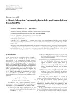
4. SIMULATIONS

In this section, we present some simulations of the proposed
technique in MATLAB environment, to assess its advantages
over the standard technique when narrowband input signals
are considered. The technique has been applied to a pipeline
ADC with 14-bit nominal resolution, to calibrate the first
stage where an error on the radix R has been forced. Monte
Carlo iterations have been performed for the parameter R
varying in a suitable range (a Gaussian distribution with a
0.2% standard deviation has been assumed).
We have considered an input signal composed of 8 tones
around the center of the Nyquist bandwidth. The random
sequence is generated from a PRBS 2
32
− 1, according to the
method described in the previous section, choosing L
= 10
(this corresponds to a bandwidth f
N
of about 0.035% of
the Nyquist bandwidth); for comparison, the same PRBS has
been used as the random signal P
N
in a standard implemen-
tation of the calibration procedure.
The use of a colored noise sequence allows to have a much
lower estimation error for the same bandwidth of the filter,
as is shown in Figure 8, that reports the transient response
of the estimation, respectively, for the standard implementa-
tion and for the proposed implementation (the initial esti-
PRBS

(2
N
)−1
Shift reg. L bit
CK
AND
CK
TQ
P
N
Figure 6: Generation of a colored random sequence.
10.90.80.70.60.50.40.30.20.10
Normalized frequency
White noise level
−120
−100
−80
−60
−40
−20
0
Power (dB)
Figure 7: Power density spectrum of the colored noise for L = 9.
mate of the radix is zero, and 100 Monte Carlo iterations are
reported). In this case, the same filter bandwidth (21 ppm of
the Nyquist bandwidth) enables a large reduction in SCNR
for the same calibration speed.
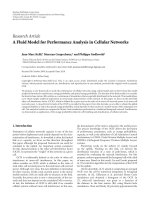
Figure 9 shows the transient response when a 100-times
larger lowpass filter is used for the proposed implementa-
tion: this allows a faster convergence of the estimation, with

a lower residue error than for the standard implementation
(note the different scale on x-axis). Despite the 100-times
faster filter, SCNR still seems lower than in the standard case.
The lower estimation error of the proposed calibration
technique allows a better calibration with lower noise. To ver-
ify this, we have simulated a pipeline ADC with 14 nominal
bits of resolution, composed of 13 identical 1.5-bit stages.
Eachstagehasgainerrorswithavarianceof1%,offset errors
(for the MDAC and the comparators) of 1%, and third-order
nonlinearity at the output of the MDAC stage with a variance
of 0.1%. This results in variance of the radix of about 1.75%,
and some nonlinear error. The input signal is composed of
four nonmodulated carriers around f
s
/4; they have the same
amplitude, which is a quarter of the full scale range of the
ADC. The gain K used for calibration has been set to 2
−18
,
and the colored random sequences have been obtained using
L
= 9. Calibration has been applied to the first four stages.
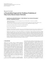
Figure 10 shows the spectrum of the output signal with-
out calibration and when calibrated with the standard and
proposed simulation technique. The same filter with band-
width of 5.4 ppm of the Nyquist frequency is used, and the
Francesco Centurelli et al. 7
4035302520151050
×10
2

Normalized time
−120
−100
−80
−60
−40
−20
0
20
40
60
Relative error (%)
(a)
4035302520151050
×10
2
Normalized time
−120
−100
−80
−60
−40
−20
0
20
40
60
Relative error (%)
(b)
Figure 8: Transient response of the standard (a) and proposed (b) method, for the same bandwidth of the estimation filter (100 Monte

Carlo iterations).
80706050403020100
×10
2
Normalized time
−120
−100
−80
−60
−40
−20
0
20
40
60
Relative error (%)
(a)
80706050403020100
Normalized time
−120
−100
−80
−60
−40
−20
0
20
40
60
Relative error (%)

(b)
Figure 9: Transient response of the standard (a) and proposed (b) method, when a 100-times larger lowpass filter is used (100 Monte Carlo
iterations).
colored sequence presents a noise floor of about 20 dB lower
than the white noise level.
Figure 11 shows the histograms of the effective number
of bits (ENOB) with and without calibration, for 100 Monte
Carlo iterations, and Table 2 reports the average value and
standard deviation of ENOB and SFDR.
Figure 12 shows the transient evolution of the ENOB as
the ADC gets calibrated: the same filter bandwidth is used
in both cases, providing the same convergence time, with a
different estimation noise, thus a different ADC precision.
In the standard calibration case, the chosen bandwidth re-
sults in an excessive calibration noise, due to the undesidered
8 EURASIP Journal on Advances in Signal Processing
10.80.60.40.20
Normalized frequency
−110
−100
−90
−80
−70
−60
−50
−40
−30
−20
−10
Amplitude (dB)

(a)
10.80.60.40.20
Normalized frequency
−110
−100
−90
−80
−70
−60
−50
−40
−30
−20
−10
Amplitude (dB)
(b)
10.80.60.40.20
Normalized frequency
−110
−100
−90
−80
−70
−60
−50
−40
−30
−20
−10
Amplitude (dB)

(c)
Figure 10: Output spectrum of the ADC: (a) output signal without calibration; (b) with standard calibration; (c) with the proposed cali-
bration.
98765
ENOB
0
2
4
6
8
10
12
14
16
18
20
(a)
109876
ENOB
0
5
10
15
20
25
(b)
12111098
ENOB
0
5

10
15
20
25
30
(c)
Figure 11: ENOB histograms: (a) without calibration; (b) standard calibration; (c) proposed calibration.
Francesco Centurelli et al. 9
1614121086420
×10
6
Number of cycles
6.5
7
7.5
8
8.5
9
9.5
10
10.5
ENOB
Proposed calibration
Standard calibration
Without calibration
Figure 12: Transient evolution of the ENOB during calibration
(same filter for standard and proposed calibration).
Table 2: Precision performance of the ADC.
No. Standard Proposed
calibration calibration calibration

ENOB: mean 6.9 bits 7.8 bits 10.5 bits
ENOB: std 0.8 bits 0.6 bits 0.6 bits
SFDR: mean 48 dB 54 dB 68 dB
SFDR: std 5.4 dB 4.3 dB 4.2 dB
terms in (11) and in particular to the input signal. If the es-
timation noise is comparable with the error term to be esti-
mated, calibration does not improve linearity, and the ENOB
presents wide oscillations around its average value.
Figure 13 shows the spectrum of V
IN
P
N
in case of a white
PRBS and a colored noise sequence: a 20 dB improvement in
the power at low frequencies, which results in the error term
(13), is evident.
If a smaller filter bandwidth is used in the standard cali-
bration case, we get a slower convergence with a smaller er-
ror. Figure 14 shows the transient evolution of the ENOB
when the gain K is 2
−16
for the proposed method and 2
−20
for the standard calibration, that results in a factor 16 on the
filter bandwidth.
5. COMPARISON WITH EXISTING TECHNIQUES
Different techniques have been presented in the literature to
improve the convergence speed of the calibration procedure
by cancellation of the interference due to the input signal.
In [9, 10] the input signal is cancelled by using two identi-

cal half-sized pipeline A/D converters in parallel, fed by the
same signal, and by extracting the error terms by filtering
off the difference between the two channels’ outputs. If the
two channels are identical, cancellation of the input interfer-
ence term is perfect, and calibration can be done much faster;
however, if the two channels are mismatched, cancellation is
incomplete and the interference term is attenuated but not
cancelled. Sensitivity to channel mismatches limits in prac-
tice the appeal of this technique: whereas the ADCs could
be scaled to exploit the calibration to achieve good accu-
racy with low area and power consumption, this increases the
mismatch between the channels reducing the effectiveness
of the calibration technique. Moreover, half-sizing the two
channels would worsen the mismatch, so that larger stages
would have to be used, with an increase in area and power
consumption with respect to a simple ADC. This issue has
beenaddressedin[14] by using a gain and offset correction
loop, in conjunction with the calibration loops, to maximize
the symmetry between the two channels.
Acompletelydifferent technique, employed in [11],
makes use of Lagrange interpolation to estimate the value of
the input signal and cancel its effect on the error estimation
process. This is done by calibrating the pipeline once every
M + 1 samples (M
= 19 in that paper) and using the previ-
ous and the successive M samples for the estimation, by using
an FIR filter to implement the interpolation. Despite the fact
that most samples are not used for calibration, a faster con-
vergence is achieved because interpolation cancels most of
the interference due to the input signal. However, this tech-

nique can be successfully used only if interpolation is accu-
rate, and this imposes more stringent conditions on the input
signal than simply to be band-limited. Moreover, the tech-
nique requires additional digital hardware, including a FIR
filter for the interpolation.
In [14] a signal dependent PRBS is employed to avoid
over-range after the PRBS insertion and to improve the num-
ber of samples that can be used in the estimation procedure,
since in most techniques calibration is possible only if the
input signal sample is contained in certain intervals, so that
many samples may be useless for the parameter estimation.
However, this technique requires additional capacitors, with
an increase in the number of error parameters to be esti-
mated.
The main limitation of the proposed technique is that the
product of two different colored PRBS will have power con-
centrated around DC, so that it will be difficult to filter out.
While the input-dependent power is mainly concentrated
outside the bandwidth of the calibration filter, the terms due
to the products among different colored PRBS will be mainly
concentrated in that frequency region. However, these prod-
ucts are proportional to the error estimate, so that they are in
general much smaller than the term given by the input signal.
While it is possible to obtain a 25–30 dB of reduction in the
power of the input-dependent term, the mixed terms will be
amplified by a similar amount. Figure 15 shows the spectrum
of the product of two noise sequences, in case of white and
colored spectra.
6. CONCLUSION
A modification to the background calibration procedure by

correlation has been presented, that allows faster conver-
gence with lower estimation errors. The technique can be
applied when the input signal to the ADC does not contain
10 EURASIP Journal on Advances in Signal Processing
10.80.60.40.20.10
Normalized frequency
−100
−90
−80
−70
−60
−50
−40
−30
−20
Amplitude (dB)
(a)
10.80.60.40.20.10
Normalized frequency
−100
−90
−80
−70
−60
−50
−40
−30
−20
Amplitude (dB)
(b)

Figure 13: Power density spectrum of P
N
V
i
: (a) white noise; (b) colored sequence.
1614121086420
×10
6
Number of cycles
6
6.5
7
7.5
8
8.5
9
9.5
10
10.5
11
ENOB
Proposed calibration
Standard calibration
Without calibration
Figure 14: Transient evolution of the ENOB during calibration.
information around dc or f
S
/2, and requires the use of a
colored random sequence instead of a white sequence. This
improves the SCNR of the estimation of the calibration pa-

rameter, and allows more flexibility in the choice of the low-
pass filter used for the estimation. A practical circuit to gen-
erate a random sequence with the desired spectral proper-
ties has been proposed, that provides a more efficient imple-
mentation than lowpass filter in a PRBS signal. Monte Carlo
10.80.60.40.20
Normalized frequency
White noise
Colored noise
−100
−90
−80
−70
−60
−50
−40
−30
−20
−10
0
Amplitude (dB)
Figure 15: Spectrum of the product of two random sequences.
simulations in Matlab show the advantages of the proposed
method both in terms of estimation error and in improve-
ment of the SFDR.
The proposed calibration technique is very simple to im-
plement, requiring only additional combinational logic with
respect to the technique by Moon and Li to generate the col-
ored random sequence, and does not impose limitations on
the input signals to the converter, a part from a little band-

width penalty on the analog bandwidth.
Francesco Centurelli et al. 11
REFERENCES
[1] J. Sevenhans and Z Y. Chang, “A/D and D/A conversion
for telecommunication,” IEEE Circuits and Devices Magazine,
vol. 14, no. 1, pp. 32–42, 1998.
[2] Y M. Lin, B. Kim, and P. R. Gray, “A 13-b 2.5-MHz self-
calibrated pipelined A/D converter in 3-μm CMOS,” IEEE
Journal of Solid-State Circuits, vol. 26, no. 4, pp. 628–636, 1991.
[3] H S. Lee, “A 12-b 600 ks/s digitally self-calibrated pipelined
algorithmic ADC,” IEEE Journal of Solid-State Circuits, vol. 29,
no. 4, pp. 509–515, 1994.
[4] S U. Kwak, B S. Song, and K. Bacrania, “A 15-b, 5-Msample/s
low-spurious CMOS ADC,” IEEE Journal of Solid-State Cir-
cuits, vol. 32, no. 12, pp. 1866–1875, 1997.
[5] O. E. Erdo
˘
gan, P. J. Hurst, and S. H. Lewis, “A 12-b digital-
background-calibrated algorithmic ADC with -90-dB THD,”
IEEE Journal of Solid-State Circuits, vol. 34, no. 12, pp. 1812–
1820, 1999.
[6] J. M. Ingino and B. A. Wooley, “A continuously calibrated 12-
b, 10-MS/s, 3.3-V A/D converter,” IEEE Journal of Solid-State
Circuits, vol. 33, no. 12, pp. 1920–1931, 1998.
[7] I. Galton, “Digital cancellation of D/A converter noise in
pipelined A/D converters,” IEEE Transactions on Circuits and
Systems II, vol. 47, no. 3, pp. 185–196, 2000.
[8] J. Ming and S. H. Lewis, “An 8-bit 80-Msample/s pipelined
analog-to-digital converter with background calibration,”
IEEE Journal of Solid-State Circuits, vol. 36, no. 10, pp. 1489–

1497, 2001.
[9] J. Li and U K. Moon, “Background calibration techniques
for multistage pipelined ADCs with digital redundancy,” IEEE
Transactions on Circuits and Systems II, vol. 50, no. 9, pp. 531–
538, 2003.
[10] J. McNeill, M. C. W. Coln, and B. J. Larivee, ““Split ADC”
architecture for deterministic digital background calibration
of a 16-bit 1-MS/s ADC,” IEEE Journal of Solid-State Circuits,
vol. 40, no. 12, pp. 2437–2445, 2005.
[11] R. G. Massolini, G. Cesura, and R. Castello, “A fully digital
fast convergence algorithm for nonlinearity correction in mul-
tistage ADC,” IEEE Transactions on Circuits and Systems II,
vol. 53, no. 5, pp. 389–393, 2006.
[12] S. H. Lewis and P. R. Gray, “ A pipelined 5-Msample/s 9-bit
analog-to-digital converter,” IEEE Journal of Solid-State Cir-
cuits, vol. 22, no. 6, pp. 954–961, 1987.
[13] J. Rajski, N. Tamarapalli, and J. Tyszer, “Automated synthe-
sis of phase shifters for built-in self-test applications,” IEEE
Transactions on Computer-Aided Design of Integrated Circuits
and Systems, vol. 19, no. 10, pp. 1175–1188, 2000.
[14] J L. Fan, C Y. Wang, and J T. Wu, “A robust and fast digital
background calibration technique for pipelined ADCs,” IEEE
Transactions on Circuits and Syste ms I, vol. 54, no. 6, pp. 1213–
1223, 2007.