Báo cáo hóa học: " Research Article Code Design for Multihop Wireless Relay Networks" pptx

Hindawi Publishing Corporation
EURASIP Journal on Advances in Signal Processing
Volume 2008, Article ID 457307, 12 pages
doi:10.1155/2008/457307
Research Article
Code Design for Multihop Wireless Relay Networks
Fr
´
ed
´
erique Oggier and Babak Hassibi
Department of Electr ical Engineering, California Institute of Technology, Pasadena CA 91125, USA
Correspondence should be addressed to F. Oggier,
Received 2 June 2007; Revised 21 October 2007; Accepted 25 November 2007
Recommended by Keith Q. T. Zhang
We consider a wireless relay network, where a transmitter node communicates with a receiver node with the help of relay nodes.
Most coding strategies considered so far assume that the relay nodes are used for one hop. We address the problem of code design
when relay nodes may be used for more than one hop. We consider as a protocol a more elaborated version of amplify-and-
forward, called distributed space-time coding, where the relay nodes multiply their received signal with a unitary matrix, in such a
way that the receiver senses a space-time code. We first show that in this scenario, as expected, the so-called full-diversity condition
holds, namely, the codebook of distributed space-time codewords has to be designed such that the difference of any two distinct
codewords is full rank. We then compute the diversity of the channel, and show that it is given by the minimum number of relay
nodes among the hops. We finally give a systematic way of building fully diverse codebooks and provide simulation results for their
performance.
Copyright © 2008 F. Oggier and B. Hassibi. This is an open access article distributed under the Creative Commons Attribution
License, which permits unrestricted use, distribution, and reproduction in any medium, provided the original work is properly
cited.
1. INTRODUCTION
Cooperative diversity is a popular coding technique for wire-
less relay networks [1]. When a transmitter node wants
to communicate with a receiver node, it uses its neigh-

bor nodes as relays, in order to get the diversity known
to be achieved by MIMO systems. Intuitively, one can
think of the relay nodes playing the role of multiple anten-
nas. What the relays perform on their received signal de-
pends on the chosen protocol, generally categorized between
amplify-and-forward (AF) and decode-and-forward (DF).
In order to evaluate their proposed cooperative schemes (for
either strategy), several authors have adopted the diversity-
multiplexing gain tradeoff proposed originally by Zheng and
Tse for the MIMO channel, for single or multiple antenna
nodes [2–5].
As specified by its name, AF protocols ask the relay nodes
to just forward their received signal, possibly scaled by a
power factor. Distributed space-time coding [6]canbeseen
as a sophisticated AF protocol, where the relays perform on
their received vector signal a matrix multiplication instead of
a scalar multiplication. The receiver thus senses a space-time
code, which has been “encoded” by both the transmitter and
the relay nodes with their matrix multiplication.
Extensive work has been done on distributed space-time
coding since its introduction. Different code designs have
been proposed, aiming at improving either the coding gain,
the decoding, or the implementation of the scheme [7–10].
Scenarios where different antennas are available have been
considered in [11, 12].
Recently, distributed space-time coding has been com-
bined with differential modulation to allow communication
over relay channels with no channel information [13–15].
Schemes are also available for multiple antennas [16].
Finally, distributed space-time codes have been consid-

ered for asynchronous communication [17].
In this paper, we are interested in considering distributed
space-time coding in a multihop setting. The idea is to
iterate the original two-step protocol: in a first step, the
transmitter broadcasts the signal to the relay nodes. The
relays receive the signal, multiply it by a unitary matrix,
and send it to a new set of relays, which do the same,
and forward the signal to the final receiver. Some multihop
protocols have been recently proposed in [18, 19], for the
amplify-and-forward protocol. Though we will give in detail
most steps with a two-hop protocol for the sake of clarity,
we will also emphasize how each step is generalized to more
hops.
2 EURASIP Journal on Advances in Signal Processing
The paper is organized as follows. In Section 2,we
present the channel model, for a two-hop channel. We then
derive a Chernoff bound on the pairwise probability of
error (Section 3), which allows us to derive the full-diversity
condition as a code design criterion. We further compute the
diversity of the channel, and show that if we have a two-hop
network, with R
1
relay nodes at the first hop, and R
2
relay
nodes at the second hop, then the diversity of the network is
min(R
1
, R
2

). Section 4 is dedicated to the code construction
itself, and some examples of proposed codes are simulated in
Section 5.
2. A TWO-HOP RELAY NETWORK MODEL
Let us start by describing precisely the three-step transmis-
sion protocol, already sketched above, that allows communi-
cation for a two-hop wireless relay network. It is based on the
twostepprotocolof[6].
We assume that the power available in the network is, re-
spectively, P
1
T, P
2
T,andP
3
T at the transmitter, at the first
hop relays, and at the second hop relays for T-time trans-
mission. We denote by A
i
∈ C
T×T
, i = 1, ,R
1
, the unitary
matrices that the first hop relays will use to process their re-
ceived signal, and by B
j
∈ C
T×T
, j = 1, , R

2
, those at the
second hop relays. Note that the matrices A
i
, i = 1, , R
1
,
B
j
, j = 1, , R
2
, are computed beforehand, and given to the
relays prior to the beginning of transmission. They are then
used for all the transmission time.
Remark 1 (the unitary condition). Note that the assumption
that the matrices have to be unitary has been introduced in
[6] to ensure equal power among the relays, and to keep the
forwarded noise white. It has been relaxed in [4].
Theprotocolisasfollows.
(1) The transmitter sends its signal s
∈ C
T
such that
E[s
∗
s] = 1. (1)
(2) The ith relay during the first hop receives
r
i
=


P
1
T
  
c
1
f
i
s + v
i
∈ C
T
, i = 1, , R
1
,(2)
where f
i
denotes the fading from the transmitter to the ith
relay, and v
i
the noise at the ith relay.
(3) The jth relay during the second hop receives
x
j
= c
2
R
1


i=1
g
ij
A
i

c
1
f
i
s + v
i

+ w
j
∈ C
T
,
= c
1
c
2

A
1
s, , A
R
1
s


⎡
⎢
⎢
⎣
f
1
g
1j
.
.
.
f
R
1
g
R
1
j
⎤
⎥
⎥
⎦
+ c
2
R
1

i=1
g
ij

A
i
v
i
+ w
j
, j = 1, , R
2
,
(3)
where g
ij
denotes the fading from the ith relay in the first hop
to the jth relay in the second hop. The normalization factor
c
2
guarantees that the total energy used at the first hop relays
is P
2
T (see Lemma 1). The noise at the jth relay is denoted
by w
j
.
(4)Atthereceiver,wehave
y
= c
3
R
2


j=1
h
j
B
j
x
j
+ z ∈ C
T
= c
3
c
2
c
1
R
2

j=1
h
j
B
j

A
1
s, , A
R
1
s


⎡
⎢
⎢
⎣
f
1
g
1j
.
.
.
f
R
1
g
R
1
j
⎤
⎥
⎥
⎦
+ c
3
R
2

j=1
h

j
B
j

c
2
R
1

i=1
g
ij
A
i
v
i
+ w
j

+ z
= c
3
c
2
c
1

B
1
A

1
s, , B
1
A
R
1
s, , B
R
2
A
1
s, , B
R
2
A
R
1
s

  
S∈C
T×R
1
R
2
×
⎡
⎢
⎢
⎢

⎢
⎢
⎢
⎢
⎢
⎢
⎢
⎢
⎢
⎢
⎢
⎣
f
1
g
11
h
1
.
.
.
f
R
1
g
R
1
1
h
1

.
.
.
f
1
g
1R
2
h
R
2
.
.
.
f
R
1
g
R
1
R
2
h
R
2
⎤
⎥
⎥
⎥
⎥

⎥
⎥
⎥
⎥
⎥
⎥
⎥
⎥
⎥
⎥
⎦

 
H∈C
R
1
R
2
×1
+ c
3
c
2
R
1

i=1
R
2


j=1
h
j
g
ij
B
j
A
i
v
i
+ c
3
R
2

j=1
h
j
B
j
w
j
+ z
  
W∈C
T×1
,
(4)
where h

j
denotes the fading from the jth relay to the receiver.
The normalization factor c
3
(see Lemma 1) guarantees that
the total energy used at the first hop relays is P
3
T. The noise
at the receiver is denoted by z.
In the above protocol, all fadings and noises are assumed
to be complex Gaussian random variables, with zero mean
and unit variance.
Though relays and transmitters have no knowledge of the
channel, we do assume that the channel is known at the re-
ceiver. This makes sense when the channel stays roughly the
same long enough so that communication starts with a train-
ing sequence, which consists of a known code. Thus, instead
of decoding the data, the receiver gets knowledge of the chan-
nel H, since it does not need to know every fading indepen-
dently.
Lemma 1. The normalization factors c
2
and c
3
are, respec-
tively, given by
c
2
=


P
2
P
1
+1
,
c
3
=

P
3
P
2
R
1
+1
.
(5)
F. Oggier and B. Hassibi 3
Proof. (1) Since E[r
∗
i
r
i
] = (P
1
+1)T, we have that
E


c
2
2

A
i
r
i

∗
A
i
r
i

=
P
2
T ⇐⇒ c
2
2

P
1
+1

T = P
2
T
⇐⇒ c

2
=

P
2
P
1
+1
.
(6)
(2) We proceed similarly to compute the power at the sec-
ond hop. We have
E

x
∗
j
x
j

=
E

c
2
2

R
1


i=1
g
ij
A
i
r
i

∗

R
1

k=1
g
kj
A
k
r
k

+ E

w
∗
j
w
j

=

c
2
2
R
1

i=1
E

r
∗
i
r
i

+ T =

P
2
R
1
+1

T,
(7)
so that
E

c
2

3

B
j
x
j

∗
B
j
x
j

=
P
3
T ⇐⇒ c
2
3

P
2
R
1
+1

T = P
3
T
⇐⇒ c

3
=

P
3
P
2
R
1
+1
.
(8)
Note that from (4), the channel can be summarized as
y
= c
1
c
2
c
3
SH + W,(9)
which has the form of a MIMO channel. This explains the
terminology distributed space-time coding, since the code-
word S has been encoded in a distributed manner among the
transmitter and the relays.
Remark 2 (generalization to more hops). Note furthermore
the shape of the channel matrix H. Each row describes a path
from the transmitter to the receiver. More precisely, each row
is of the form f
i

g
ij
h
j
, which gives the path from the trans-
mitter to the ith relay in the first hop, then from the ith relay
to the jth relay in the second hop, and finally from the jth
relay to the receiver. Thus, though we have given the model
for a two-hop network, the generalization to more hops is
straightforward.
3. PAIRWISE ERROR PROBABILITY
In this section, we compute a Chernoff bound on the pair-
wise probability of error of transmitting a signal s,andde-
coding a wrong signal. The goal is to derive the so-called
diversity property as code-design criterion (Section 3.1). We
then further elaborate the upper bound given by the Cher-
noff bound, and prove that the diversity of a two-hop re-
lay network is actually min(R
1
, R
2
), where R
1
and R
2
are the
number of relay nodes at the first and second hops, respec-
tively, (Section 3.2).
In the following, the matrix I denotes the identity matrix.
3.1. Chernoff bound on the pairwise error probability

In order to determine the maximum likelihood decoder, we
first need to compute
P

y | s, f
i
, g
ij
, h
j

. (10)
If g
ij
and h
j
are known, then W is Gaussian with zero mean.
Thus knowing f
i
, g
ij
, h
j
, H and s, we know that y is Gaussian.
(1) The expectation of y given s and H is
E[y]
= c
1
c
2

c
3
SH. (11)
(2) Thevariance of y given g
ij
and h
j
is
E

y −E[y]

y −E[y]

∗

=
E

WW
∗

=
c
2
3
c
2
2
E


R
1

i=1
R
2

j=1
h
j
g
ij
B
j
A
i
v
i
R
1

k=1
R
2

l=1

h
l

g
kl
B
l
A
k
v
k

∗

+ c
2
3
E

R
2

j=1
h
j
B
j
w
j
R
2

l=1


h
l
B
l
w
l

∗

+ E

zz
∗

=
c
2
3
c
2
2
R
1

i=1

R
2


j=1
g
ij
h
j
B
j

R
2

l=1
g
∗
il
h
∗
l
B
∗
l

+ c
2
3
R
2

j=1



h
j


2
I
T
+ I
T
=: R
y
,
(12)
where
c
2
2
c
2
3
=
P
2
P
3

P
1
+1


P
2
R
1
+1

. (13)
Summarizing the above computation, we obtain the obvious
following proposition.
Proposition 1.
P

y | s, f
i
, g
ij
, h
j

=
1
π
T
det

R
y

exp


−

y −c
1
c
2
c
3
SH

∗
×R
−1
y

y−c
1
c
2
c
3
SH

.
(14)
Thus the maximum likelihood (ML) decoder of the sys-
tem is given by
arg max
s

P

y | s, f
i
, g
ij
, h
j

=
arg min
s


y −c
1
c
2
c
3
SH


2
.
(15)
From the ML decoding rule, we can compute the pairwise
error probability (PEP).
Lemma 2 (Chernoff bound on the PEP). The PEP of send-
ing a signal s

k
anddecodinganothersignals
l
has the following
Chernoff bound:
P

s
k
−→ s
l

≤
E
f
i
,g
ij
,h
j
exp

−
1
4
c
2
1
c
2

2
c
2
3
H
∗
×

S
k
−S
l

∗
R
−1
y

S
k
−S
l

H

.
(16)
4 EURASIP Journal on Advances in Signal Processing
Proof. By definition,
P


s
k
−→ s
l
| f
i
, g
ij
, h
j

=
P

P(y | s
l
, f
i
, g
ij
, h
j

>P

y | s
k
, f
i

, g
ij
, h
j

=
P

ln

P(y | s
l
, f
i
, g
ij
, h
j

−
ln

P

y | s
k
, f
i
, g
ij

, h
j

> 0

≤
E
W

expλ

ln

P

y | s
l
, f
i
, g
ij
, h
j

−
ln

P

y | s

k
, f
i
, g
ij
, h
j

,
(17)
where the last inequality is obtained by applying the Chernoff
bound, and λ>0. Using Proposition 1,wehave
λ

ln

P

y | s
l
, f
i
, g
ij
, h
j

−ln

P


y | s
k
, f
i
, g
ij
, h
j

=−
λ

c
2
1
c
2
2
c
2
3
H
∗

S
∗
K
−S
∗

l

R
−1
y

S
k
−S
l

H + c
1
c
2
c
3
H
∗
×

S
∗
K
−S
∗
l

R
−1

y
W +c
1
c
2
c
3
W
∗
R
−1
y

S
k
−S
l

H

=−

λc
1
c
2
c
3

S

k
−S
l

H + W

∗
×R
−1
y

λc
1
c
2
c
3

S
k
−S
l

H + W

+

λ
2
−λ


c
2
1
c
2
2
c
2
3
H
∗

S
k
−S
l

∗
R
−1
y

S
k
−S
l

H
+ W

∗
R
−1
y
W,
(18)
and thus
E
W

expλ

ln

P(y | s
l
, f
i
, g
ij
, h
j

−
ln

P

y | s
k

, f
i
, g
ij
, h
j

=

exp

−W
∗
R
−1
W
W

π
T
det

R
−1
W

expλ

ln


P

y | s
l
, f
i
, g
ij
, h
j

−
ln

P

y | s
k
, f
i
, g
ij
, h
j

dW
= exp

λ
2

−λ

c
2
1
c
2
2
c
2
3
H
∗

S
k
−S
l

∗
R
−1
y

S
k
−S
l

H


(19)
since R
w
= R
y
and
1
π
T
det

R
−1
W


exp

−

λc
1
c
2
c
3

S
k

−S
l

H + W

∗
×R
−1
y

λc
1
c
2
c
3

S
k
−S
l

H + W

×
dW = 1.
(20)
To conclude, we choose λ
= 1/2, which maximizes λ
2

− λ,
and thus minimizes
−(λ −λ
2
).
We now compute the expectation over f
i
. Note that one
has to be careful since the coefficients f
i
arerepeatedinthe
matrix H, due to the second hop.
Lemma 3 (bound by integrating over f). The following upper
bound holds on the PEP:
P

s
k
−→ s
l

≤
E
g
ij
,h
j
det

I

R
1
+
1
4
c
2
1
c
2
2
c
2
3
H
∗

S
k
−S
l

∗
R
−1
y

S
k
−S

l

H

−1
(21)
where H is given in (22).
Proof. We first rewrite the channel matrix H as H
= H f,
with
f
=
⎡
⎢
⎢
⎣
f
1
.
.
.
f
R
1
⎤
⎥
⎥
⎦
∈ C
R

1
,
H
=
⎡
⎢
⎢
⎢
⎢
⎢
⎢
⎢
⎢
⎢
⎢
⎢
⎢
⎢
⎢
⎣
g
11
h
1
.
.
.
g
R
1

1
h
1
.
.
.
g
1R
2
h
R
2
.
.
.
g
R
1
R
2
h
R
2
⎤
⎥
⎥
⎥
⎥
⎥
⎥

⎥
⎥
⎥
⎥
⎥
⎥
⎥
⎥
⎦
∈ C
R
1
R
2
×R
1
.
(22)
Thus we have, since f is Gaussian with 0 mean and variance
I
R
1
,
E
f
i
exp

−
1

4
c
2
1
c
2
2
c
2
3
H
∗

S
k
−S
l

∗
R
−1
y

S
k
−S
l

H


=

exp

−f
∗
f

π
R
1
exp

−
1
4
c
2
1
c
2
2
c
2
3
f
∗
H
∗


S
k
−S
l

∗
×R
−1
y

S
k
−S
l

H f

df
=
1
π
R
1

exp

−
f
∗


I
R
1
+
1
4
c
2
1
c
2
2
c
2
3
H
∗

S
k
−S
l

∗
×R
−1
y

S
k

−S
l

H

f

df
= det

I
R
1
+
1
4
c
2
1
c
2
2
c
2
3
H
∗

S
k

−S
l

∗
×R
−1
y

S
k
−S
l

H

−1
.
(23)
Similarly to the standard MIMO case, and to the previous
work on distributed space-time coding [6], the full-diversity
condition can be deduced from (21).Inordertoseeit,we
first need to determine the dominant term as a function of P,
the power used for the whole network.
Remark 3 (power allocation). In this paper, we assume that
the power P is shared equally among the transmitter and the
three hops, namely,
P
1
=
P

3
, P
2
=
P
3R
1
, P
3
=
P
3R
2
. (24)
It is not clear that this strategy is the best, however, it is a
priori the most natural one to try. Under this assumption,
we have that
c
2
3
=
P
R
2
(P +3)
,
c
2
2
c

2
3
=
P
2
R
1
R
2
(P +3)
2
,
c
2
1
c
2
2
c
2
3
=
P
3
T
3R
1
R
2
(P +3)

2
.
(25)
Thus, when P grows, c
2
1
c
2
2
c
2
3
grows like P.
F. Oggier and B. Hassibi 5
Remark 4 (full diversity). It is now easy to see from (21) that
if S
l
−S
k
drops rank, then the exponent of P increases, so that
the diversity decreases. In order to minimize the Chernoff
bound, one should then design distributed space-time codes
such that det (S
k
−S
l
)
∗
(S
k

− S
l
)=0 (property well known as
full diversity). Note that the term R
−1
y
between S
k
− S
l
and
its conjugate does not interfere with this reasoning, since R
y
can be upper bounded by tr(R
y
)I (see also Proposition 2 for
more details). Finally, the whole computation that yields to
the full-diversity criterion does not depend on H being the
channel matrix of a two-hop protocol, since the decomposi-
tion of H used in the proof of Lemma 3 could be done simi-
larly if there were three hops or more.
3.2. Diversity analysis
The goal is now to show that the upper bound given in (21)
behaves like P
min(R
1
,R
2
)
when we let P grows. To do so, let us

start by further bounding the pairwise error probability.
Proposition 2. Assumingthatthecodeisfullydiverse,itholds
that the PEP can be upper bounded as follows:
P

s
k
−→ s
l

≤
E
g
ij
,h
j
R
1

i=1
×

1+
λ
2
min
c
2
1
c

2
2
c
2
3
4T
×

R
2
j=1


h
j


2


g
ij


2
c
2
3
c
2

2

R
1
k=1




R
2
j=1
h
j
g
kj



2
+c
2
3

R
2
j=1


h

j


2
+1

−1
≤E
g
ij
,h
j
R
1

i=1
×

1+
λ
2
min
c
2
1
c
2
2
c
2

3
4T
×

R
2
j=1
|h
j
g
ij
|
2
c
2
3
c
2
2
(2R
2
−1)

R
1
k=1

R
2
j=1

|h
j
g
kj
|
2
+c
2
3

R
2
j=1
|h
j
|
2
+1

−1
.
(26)
Proof. (1) Note first that
R
y
≤tr

R
y


I
T
=

c
2
3
c
2
2
R
1

i=1
tr

R
2

j=1
g
ij
h
j
B
j
R
2

l=1

g
∗
il
h
∗
l
B
∗
l


 
α
+ T

c
2
3
R
2

j=1


h
j


2
+1


I
T
,
(27)
so that
P

s
k
−→ s
l

≤
E
g
ij
,h
j
det

I
R
1
+
c
2
1
c
2

2
c
2
3
4

c
2
3
c
2
2
α + T

c
2
3

R
2
j=1


h
j


2
+1


×
H
∗

S
k
−S
l

∗

S
k
−S
l

H

−1
≤E
g
ij
,h
j
det

I
R
1
+

λ
2
min
c
2
1
c
2
2
c
2
3
4

c
2
3
c
2
2
α+T

c
2
3

R
2
j=1



h
j


2
+1

H
∗
H

−1
,
(28)
where λ
2
min
denote the smallest eigenvalue of (S
k
−S
l
)
∗
(S
k
−
S
l
), which is strictly positive under the assumption that the

codebook is fully diverse.
Furthermore, we have that
H
∗
H =
R
2

j=1
⎛
⎜
⎜
⎜
⎝


h
j


2


g
1j


2
.
.

.


h
j


2


g
R
1
j


2
⎞
⎟
⎟
⎟
⎠
=
⎛
⎜
⎜
⎜
⎜
⎜
⎜

⎜
⎜
⎜
⎝
R
2

j=1


h
j


2


g
1j


2
.
.
.
R
2

j=1



h
j


2


g
R
1
j


2
⎞
⎟
⎟
⎟
⎟
⎟
⎟
⎟
⎟
⎟
⎠
,
(29)
which yields
det


I
R
1
+
λ
2
min
c
2
1
c
2
2
c
2
3
4

c
2
3
c
2
2
α+T

c
2
3


R
2
j=1


h
j


2
+1

H
∗
H

−1
=
R
1

i=1

1+
λ
2
min
c
2

1
c
2
2
c
2
3
4

c
2
3
c
2
2
α+T

c
2
3

R
2
j=1


h
j



2
+1

R
2

j=1


h
j


2


g
ij


2

−1
,
(30)
where
α
≤|α|
=






R
1

k=1
tr

R
2

j=1
g
kj
h
j
B
j
R
2

l=1
g
∗
kl
h
∗
l

B
∗
l






≤
R
1

k=1





tr

R
2

j=1
g
kj
h
j
B

j
R
2

l=1
g
∗
kl
h
∗
l
B
∗
l






≤
R
1

k=1






tr

R
2

j,j

=1
g
kj
g
∗
kj

h
j
h
∗
j

B
j
B
∗
j


tr

R

2

l,l

=1
g
kl
g
∗
kl

h
l
h
∗
l

B
l
B
∗
l


,
(31)
where the last inequality uses Cauchy-Schwartz inequality.
Now recall that B
j
, j = 1, , R

2
, are unitary, thus B
j
B
∗
j

and
B
l
B
∗
l

are unitary matrices, and
tr

B
k
B
∗
k


≤T ∀k,k

. (32)
6 EURASIP Journal on Advances in Signal Processing
Thus
α

≤T
R
1

k=1






R
2

j,j

=1
g
kj
g
∗
kj

h
j
h
∗
j



R
2

l,l

=1
g
kl
g
∗
kl

h
l
h
∗
l


=
T
R
1

k=1











R
2

j=1
h
j
g
kj





2





R
2

l=1
h
l

g
kl





2
= T
R
1

k=1





R
2

j=1
h
j
g
kj






2
.
(33)
We c an n ow r ew rite
P(s
k
−→ s
l
)
≤E
g
ij
,h
j
R
1

i=1

1+
λ
2
min
c
2
1
c
2
2

c
2
3
4

c
2
3
c
2
2
α + T

c
2
3

R
2
j=1


h
j


2
+1

×

R
2

j=1


h
j


2


g
ij


2

−1
≤E
g
ij
,h
j
R
1

i=1
×


1+
λ
2
min
c
2
1
c
2
2
c
2
3
4

c
2
3
c
2
2
T

R
1
k=1





R
2
j=1
h
j
gk
j



2
+T

c
2
3

c
2
3

R
2
j=1


h
j



2
+1

×
R
2

j=1


h
j


2


g
ij


2

−1
,
(34)
which proves the first bound.
(2) To get the second bound, we need to prove that






R
2

j=1
h
j
g
kj





2
≤

2R
2
−1

R
2

j=1



h
j
g
kj


2
. (35)
By the triangle inequality, we have that





R
2

j=1
h
j
g
kj





2
≤


R
2

j=1


h
j
g
kj



2
=
R
2

j=1


h
j
g
kj


2
+
R

2

j=1


h
j
g
kj


R
2

l=1,l=j


h
l
g
kl


.
(36)
Using the inequality of arithmetic and geometric means, we
get


h

j
g
kj




h
l
g
kl


=



h
j
g
kj


2


h
l
g
kl



2
≤


h
j
g
kj


2
+


h
l
g
kl


2
,
(37)
so that






R
2

j=1
h
j
g
kj





2
≤
R
2

j=1


h
j
g
kj


2
+

R
2

j=1
R
2

l=1,l=j



h
j
g
kj


2
+


h
l
g
kl


2

=

R
2
R
2

j=1


h
j
g
kj


2
+
R
2

j=1
R
2

l=1,l=j


h
l
g
kl



2
=

2R
2
−1

R
2

j=1


h
j
g
kj


2
,
(38)
which concludes the proof.
We n ow se t x
i
:=

R

2
j=1
|h
j
g
ij
|
2
, so that the bound
E
g
ij
,h
j
R
1

i=1
×

1+
λ
2
min
c
2
1
c
2
2

c
2
3
4T
  
γ
1
×

R
2
j=1
|h
j
g
ij
|
2
c
2
2
c
2
3

2R
2
−1



 
γ
2

R
1
k=1

R
2
j=1
|h
j
g
kj
|
2
+c
2
3

R
2
j=1
|h
j
|
2
+1


−1
(39)
can be rewritten as
E
g
ij
,h
j
R
1

i=1

1+γ
1
x
i
γ
2

R
1
k=1
x
k
+ c
2
3

R

2
j=1


h
j


2
+1

−1
. (40)
Note here that by choice of power allocation (see Remark 3),
γ
1
=
λ
2
min
P
3
T
4T3R
1
R
2
(P +3)
2
=

λ
2
min
P
3
12R
1
R
2
(P +3)
2
,
γ
2
=

2R
2
−1

P
2
R
1
R
2
(P +3)
2
,
c

2
3
=
P
R
2
(P +3)
.
(41)
In order to compute the diversity of the channel, we will con-
sider the asymptotic regime in which P
→∞.Wewillthususe
the notation
x
.
= y ⇐⇒ lim
P→∞
x
log P
= lim
P→∞
y
log P
. (42)
With this notation, we have that
γ
1
.
= P, γ
2

.
= P
0
= 1, c
2
3
.
= P
0
= 1. (43)
In other words, the coefficients γ
2
and c
3
areconstantsand
can be neglected, while γ
1
grows with P.
Theorem 1. It holds that
E
g
ij
,h
j
R
1

i=1

1+P

x
i

R
2
k=1
x
k
+

R
2
j=1


h
j


2
+1

−1
.
= P
−min{R
1
,R
2
}

,
(44)
F. Oggier and B. Hassibi 7
where x
i
:=

R
2
j=1
|h
j
g
ij
|
2
. In other words, the diversity of the
two-hop wireless relay network is min(R
1
, R
2
).
Proof. Since we are interested in the asymptotic regime in
which P
→∞, we define the random variables α
j
, β
ij
, so that



h
j


2
=P
−α
j
,


g
ij


2
=P
−β
ij
, i=1, , R
1
, j =1, , R
2
.
(45)
We thus have that
x
i
=

R
2

j=1


h
j
g
ij


2
=
R
2

j=1
P
−(α
j
+β
ij
)
= P
max
j
{−(α
j
+β

ij
)}
= P
−min
j
{α
j
+β
ij
}
,
(46)
where the third equality comes from the fact that P
a
+ P
b
.
=
P
max{a,b}
.
Similarly (and using the same fact), we have that
R
2

k=1
x
k
+
R

2

j=1


h
j


2
+1
.
=
R
2

k=1
P
−min
j
{α
j
+β
kj
}
+
R
2

j=1

P
−α
j
+1
.
= P
max
k
(−min
j
(α
j
+β
kj
))
+ P
max
j
(−α
j
)
+1
.
= P
max(−min
jk
(α
j
+β
kj

),−min
j
α
j
)
+1.
(47)
The above change of variable implies that
d


h
j


2
= (log P)P
−α
j
dα
j
, d


g
ij


2
= (log P)P

−β
ij
dβ
ij
,
(48)
and recalling that
|h
j
|
2
and |g
2
ij
| are independent, exponen-
tially distributed, random variables with mean 1, we get
E
g
ij
,h
j
R
1

i=1

1+P
x
i


R
2
k=1
x
k
+

R
2
j=1


h
j


2
+1

−1
=

∞
0
R
1

i=1

1+P

x
i

R
2
k=1
x
k
+

R
2
j=1


h
j


2
+1

−1
×
R
1

i=1
R
2


j=1
exp

−


g
ij


2

d


g
ij


2
×
R
2

j=1
exp

−



h
j


2

d


h
j


2
=

∞
−∞
R
1

i=1

1+P
P
−min
j
{α
j

+β
ij
}
P
−min(min
jk
(α
j
+β
kj
),min
j
α
j
)
+1

−1
×
R
1

i=1
R
2

j=1
exp

−

P
−β
ij

(log P)P
−β
ij
dβ
ij
×
R
2

j=1
exp

−
P
−α
j

(log P) P
−α
j
dα
j
.
(49)
Note that to lighten the notation by a single integral, we mean
that this integral applies to all the variables. Now recall that

exp

−P
−a

.
= 0, a<0, exp

−P
−a

.
= 1, a>0,
(50)
and that
exp

−
P
−a

exp

−
P
−b

=
exp


−

P
−a
+ P
−b

.
= exp

−
P
−min(a,b)

(51)
meaning that in a product of exponentials, if at least one
of the variables is negative, then the whole product tends
to zero. Thus, only the integral where all the variables are
positive does not tend to zero exponentially, and we are
left with integrating over the range for which α
j
≥0, β
ij
≥0,
i
= 1, , R
1
, j = 1, , R
2
. This implies in particular that

P
−min(min
jk
(α
j
+β
kj
),min
j
α
j
)
+1
.
= P
−c
+1
.
= P
max(−c,0)
.
= 1
(52)
since c>0. This means that the denominator does not con-
tribute in P. Note also that the (log P)factorsdonotcon-
tribute to the exponential order.
Hence
E
g
ij

,h
j
R
1

i=1

1+P
x
i

R
2
k=1
x
k
+

R
2
j=1
|h
j
|
2
+1

−1
.
=


∞
0
R
1

i=1

1+P
1−min
j
{α
j
+β
ij
}

−1
R
1

i=1
R
2

j=1
P
−β
ij
dβ

ij
R
2

j=1
P
−α
j
dα
j
.
=

∞
0
R
1

i=1

P
(1−min
j
{α
j
+β
ij
})
+


−1
R
1

i=1
R
2

j=1
P
−β
ij
dβ
ij
R
2

j=1
P
−α
j
dα
j
=

∞
0
R
1


i=1
P
−(1−min
j
{α
j
+β
ij
})
+
R
1

i=1
R
2

j=1
P
−β
ij
dβ
ij
R
2

j=1
P
−α
j

dα
j
,
(53)
where (
·)
+
denotes max{·,0} and the second equality is ob-
tained by writing 1
= P
0
.
By Laplace’s method [20,page50],[21], this expectation
is equal in order to the dominant exponent of the integrand
E
g
ij
,h
j
R
1

i=1

1+P
x
i

R
2

k=1
x
k
+

R
2
j=1
|h
j
|
2
+1

−1
.
=

∞
0
P
−f (α
j
,β
ij
)
R
1

i=1

R
2

j=1
dβ
ij
R
2

j=1
dα
j
.
= P
−inf f (α
j
,β
ij
)
,
(54)
where
f

α
j
, β
ij

=

R
1

i=1

1 −min
j

α
j
+ β
ij


+
+
R
1

i=1
R
2

j=1
β
ij
+
R
2


j=1
α
j
.
(55)
In order to conclude the proof, we are left to show that
inf
α
j
,β
ij
f

α
j
, β
ij

=
min

R
1
, R
2

. (56)
(i) First note that if R
1
<R

2
, R
1
is achieved when α
j
= 0,
β
ij
= 0 and if R
1
>R
2
, R
2
is achieved when α
j
= 1, β
ij
= 0.
(ii) We now look at optimizing over β
ij
. Note that one
cannot optimize the terms of the sum separately. Indeed, if
8 EURASIP Journal on Advances in Signal Processing
β
ij
are reduced to make

R
1

i=1

R
2
j=1
β
ij
smaller, then the first
term increases, and vice versa. One can actually see that we
may set all β
ij
= 0 since increasing any β
ij
from zero does not
decrease the sum.
(iii) Then the optimization becomes one over the α
j
:
inf
α
j
≥0
R
1

i=1

1 −min
j


α
j


+
+
R
2

j=1
α
j
. (57)
Using a similar argument as above, note that if α
j
are taken
greater than 1, then the first term cancels, but then the sec-
ond term grows. Thus the minimum is given by considering
α
j
∈ [0, 1] which means that we can rewrite the optimization
problem as
inf
α
j
∈[0,1]
R
1

i=1


1 −min
j

α
j


+
+
R
2

j=1
α
j
. (58)
Now we have that
R
1

i=1

1 −min
j

α
j



+
R
2

j=1
α
j
= R
1

1 −min
j

α
j


+
R
2

j=1
α
j
≥ R
1

1 −min
j


α
j


+ R
2
min
j

α
j

=
R
1
+(R
2
−R
1
)min
j

α
j

.
(59)
(iv) This final expression is minimized when α
j
= 0, j =

1, , R
2
for R
1
<R
2
and α
j
= 1, j = 1, , R
2
for R
1
>R
2
,
since if R
2
−R
1
< 0, one will try to remove as much as possible
from R
1
. Since α
j
≤1, the optimal is to take α
j
= 1. Thus if
R
1
<R

2
, the minimum is given by R
1
, while it is given by
R
1
+ R
2
−R
1
= R
2
if R
2
<R
1
, which yields min{R
1
, R
2
}.
Hence inf
α
j
,β
ij
f (α
j
, β
ij

) = min{R
1
, R
2
} and we conclude
that
E
g
ij
,h
j
R
1

i=1

1+P
x
i

R
2
k=1
x
k
+

R
2
j=1

|h
j
|
2
+1

−1
.
=P
−min{R
1
,R
2
}
.
(60)
Let us now comment the interpretation of this result.
Since the diversity is also interpreted as the number of in-
dependent paths from transmitter to receiver, one intuitively
expects the diversity to behave as the minimum between R
1
and R
2
, since the bottleneck in determining the number of
independent paths is clearly min(R
1
, R
2
).
4. CODING STRATEGY

We now discuss the design of the distributed space-time code
S
=

B
1
A
1
s, , B
1
A
R
1
s, , B
R
2
A
1
s, , B
R
2
A
R
1
s

∈ C
T×R
1
R

2
.
(61)
For the code design purpose, we assume that T
= R
1
R
2
.
Remark 5. There is no loss in generality in assuming that the
distributed space-time code is square. Indeed, if one needs
a rectangular space-time code, one can always pick some
columns (or rows) of a square code. If the codebook satis-
fies that (S
k
−S
l
)
∗
(S
k
−S
l
) is fully diverse, then the codebook
obtained by removing columns will be fully diverse too (see,
e.g., [12] where this phenomenon has been considered in the
context of node failures). This will be further illustrated in
Section 5.
The coding problem consists of designing unitary matri-
ces A

i
, i = 1, , R
1
, B
j
, j = 1, , R
2
, such that S as given
in (61) is full rank, as explained in the previous section (see
Remark 4). We will show in this section how such matrices
can be obtained algebraically.
Recall that given a monic polynomial
p(x)
= p
0
+ p
1
x + ···+ p
n−1
x
n−1
+ x
n
∈ C[x], (62)
its companion matrix is defined by
C(p)
=
⎛
⎜
⎜

⎜
⎜
⎜
⎜
⎝
00··· 0 −p
0
10 0−p
1
01 0−p
2
.
.
.
.
.
.
.
.
.
0
.
.
.
00 1
−p
n−1
⎞
⎟
⎟

⎟
⎟
⎟
⎟
⎠
. (63)
Set
Q(i):={a + ib, a, b ∈ Q}, which is a subfield of the
complex numbers.
Proposition 3. Let p(x) be a monic irreducible polynomial of
degree n in
Q(i)[x], and denote by θ one of its roots. Con-
sider the vector space K of degree n over
Q(i) with basis
{1, θ, , θ
n−1
}.
(1) The matrix M
s
of multiplication by
s
= s
0
+ s
1
θ + ···+ s
n−1
θ
n−1
∈ K (64)

is of the form
M
s
=

s, C(p)s, , C(p)
n−1
s

, (65)
where s
= [s
0
, s
1
, , s
n−1
]
T
and C(p) is the companion matrix
of p(x).
(2) Furthermore,
det

M
s

=
0 ⇐⇒ s = 0. (66)
Proof. (1) By definition, M

s
satisfies

1, θ, , θ
n−1

M
s
= s

1, θ, , θ
n−1

. (67)
Thus the first column of M
s
is clearly s, since

1, θ, , θ
n−1

s = s. (68)
Now, we have that
sθ
= s
0
θ + s
1
θ
2

+ ···+ s
n−2
θ
n−1
+ s
n−1
θ
n
=−p
0
s
n−1
+ θ

s
0
− p
1
s
n−1

+ ···
+ θ
n−1

s
n−2
− p
n−1
s

n−1

(69)
F. Oggier and B. Hassibi 9
since θ
n
=−p
0
− p
1
θ −··· − p
n−1
θ
n−1
. Thus the second
column of M
s
is clearly
⎛
⎜
⎜
⎜
⎜
⎝
−
p
0
s
n−1
s

0
− p
1
s
n−1
.
.
.
s
n−2
− p
n−1
s
n−1
⎞
⎟
⎟
⎟
⎟
⎠
=
⎛
⎜
⎜
⎜
⎜
⎜
⎜
⎝
00··· 0 −p

0
10 0−p
1
01 0−p
2
.
.
.
.
.
.
.
.
.
0
.
.
.
00 1
−p
n−1
⎞
⎟
⎟
⎟
⎟
⎟
⎟
⎠
⎛

⎜
⎜
⎜
⎜
⎝
s
0
s
1
.
.
.
s
n−1
⎞
⎟
⎟
⎟
⎟
⎠
.
(70)
We have thus shown that for any s
∈ K, sθ = C(p)s.By
iterating this processing, we have that
sθ
2
= (sθ)θ = C(p)sθ = C(p)
2
s, (71)

and thus sθ
j
= C(p)
j
s is the j+1 column of M
s
, j = 1, , n−
1.
(2) Denote by θ
1
, , θ
n
the n roots of p.Letθ be any of
them. Denote by σ
j
the following Q(i)-linear map:
σ
j
(θ) = θ
j
, j = 1, , n. (72)
Now, it is clear, by definition of M
s
,namely,

1, θ, , θ
n−1

M
s

= s

1, θ, , θ
n−1

, (73)
that s is an eigenvalue of M
s
associated to the eigenvector
(1, θ, , θ
n−1
). By applying σ
j
to the above equation, we
have, by
Q(i)-linearity, that

1, σ
j
(θ), , σ
j

θ
n−1

M
s
= σ
j
(s)


1, σ
j
(θ), , σ
j

θ
n−1

.
(74)
Thus σ
j
(s)isaneigenvalueofM
s
, j = 1, , n,and
det

M
s

=
n

j=1
σ
j
(s), (75)
which concludes the proof.
The matrix M

s
, as described in the above proposition, is
a natural candidate to design a distributed space-time code,
since it has the right structure, and is proven to be fully di-
verse. However, in this setting, C(p) and its powers corre-
spond to products of A
i
B
j
, which are unitary. Thus, C(p)has
to be unitary. A straightforward computation shows the fol-
lowing.
Lemma 4. One has that C(p) is unitary if and only if
p
1
=···=p
n−1
= 0,


p
0


2
= 1. (76)
The family of codes proposed in [10] is a particular case,
when p
0
is a root of unity.

The distributed space-time code design can be summa-
rized as follow.
(1) Choose p(x) such that
|p
0
|
2
= 1andp(x)isirre-
ducible over
Q(i).
(2) Define
A
i
= C(p)
i−1
, i = 1, , R
1
,
B
j
= C(p)
R
1
(j−1)
, j = 1, , R
2
.
(77)
Example 5 (R
1

= R
2
= 2). We need a monic polynomial of
degree 4 of the form
p(x)
= x
4
− p
0
,


p
0


2
= 1. (78)
For example, one can take
p(x)
= x
4
−
i +2
i −2
, (79)
which are irreducible over
Q(i). Its companion matrix is
given by
⎛

⎜
⎜
⎜
⎜
⎝
000
i +2
i −2
100 0
010 0
001 0
⎞
⎟
⎟
⎟
⎟
⎠
. (80)
The matrices A
1
, A
2
, B
1
, B
2
are given explicitly in next sec-
tion.
Example 6 (R
1

= R
2
= 3). We need now a monic polynomial
of degree 9. For example,
p(x)
= x
9
−
i +2
i −2
, (81)
is irreducible over
Q(i), with companion matrix
⎛
⎜
⎜
⎜
⎜
⎜
⎜
⎜
⎜
⎜
⎜
⎜
⎜
⎜
⎜
⎜
⎝

00000000
i +2
i −2
10000000 0
01000000 0
00100000 0
00010000 0
00001000 0
00000100 0
00000010 0
00000001 0
⎞
⎟
⎟
⎟
⎟
⎟
⎟
⎟
⎟
⎟
⎟
⎟
⎟
⎟
⎟
⎟
⎠
. (82)
5. SIMULATION RESULTS

In this section, we present simulation results for different sce-
narios. For all plots, the x-axis represents the power (in dB)
of the whole network, and the y-axis gives the block error
rate (BLER).
Diversity discussion
In order to evaluate the simulation results, we refer to
Theorem 1. Since the diversity is interpreted both as the slope
of the error probability in log-log scale as well as the expo-
nent of P in the upper bound on the pairwise error proba-
bility, one intuitively expects the slope to behave as the min-
imum between R
1
and R
2
.
10 EURASIP Journal on Advances in Signal Processing
T
x
A
1
A
2
B
1
B
2
R
x
T
x

A
1
A
2
R
x
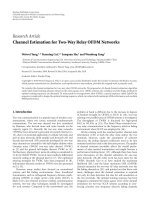
Figure 1: On the left, a two-hop network with two nodes at each
hop. On the right, a one-hop network with two nodes.
We first consider a simple network with two hops and
two nodes at each hop, as shown in the left of Figure 1.The
coding strategy (see Example 5)isgivenby
A
1
= I
4
, A
2
=
⎛
⎜
⎜
⎜
⎜
⎜
⎝
000
i +2
i −2
100 0
010 0

001 0
⎞
⎟
⎟
⎟
⎟
⎟
⎠
,
B
1
= I
4
, B
2
=
⎛
⎜
⎜
⎜
⎜
⎜
⎜
⎜
⎝
00
i +2
i −2
0
00 0

i +2
i −2
10 0 0
01 0 0
⎞
⎟
⎟
⎟
⎟
⎟
⎟
⎟
⎠
.
(83)
We have simulated the BLER of the transmitter sending a
signal to the receiver through the two hops. The results are
shown in Figure 2, given by the dashed curve. Following the
above discussion, we expect a diversity of two. In order to
have a comparison, we also plot the BLER of sending a mes-
sage through a one-hop network with also two relay nodes,
as shown on the right of Figure 1. This plot comes from [10],
where it has been shown that with one hop and two relays,
the diversity is two. The two slopes are clearly parallel, show-
ing that the two-hop network with two relay nodes at each
hop has indeed diversity of two. There is no interpretation
in the coding gain here, since in the one-hop relay case, the
power allocated at the relays is more important (half of the
total power, while one third only in the two-hop case), and
the noise forwarded is much bigger in the two-hop case. Fur-

thermore, the coding strategies are different.
We also emphasize the importance of performing coding
at the relays. Still on Figure 1, we show the performance of
doing coding either only at the first hop, or only at the second
hop. It is clear that this yields no diversity.
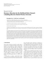
We now consider more in details a two-hop network with
three relay nodes at each hop, as show in Figure 3.Transmit-
ter and receiver for a two-hop communication are indicated
and are plotted as boxes, while the second hop also contains
a box, indicating that this relay is also able to be a transmit-
ter/receiver. We will thus consider both cases, when it is either
a relay node or a receiver node. Nodes that serve as relays are
all endowed with a unitary matrix, denoted by either A
i
at the
first hop, or B
j
for the second hop, as explained in Section 4.
BLER
10
−3
10
−2
10
−1
10
0
16 18 20 22 24 26 28 30
P (dB)
2nodes

2-2 nodes
2-2 (no) nodes
2(no)-2nodes
Figure 2: Comparison between a one-hop network with two relay
nodes and a two-hop network with two relay nodes at each hop,
“(no)” means that no coding has been done either at the first or
second hop.
T
x
A
1
A
2
A
3
B
1
B
2
B
3
R
x
Figure 3: A two-hop network with three nodes at each hop. Nodes
able to be transmitter/receiver are shown as boxes.
For the upcoming simulations, we have used the following
coding strategy (see Example 6). Set
Γ
=
⎛

⎜
⎜
⎜
⎜
⎜
⎜
⎜
⎜
⎜
⎜
⎜
⎜
⎜
⎜
⎜
⎜
⎝
00000000
i +2
i −2
10000000 0
01000000 0
00100000 0
00010000 0
00001000 0
00000100 0
00000010 0
00000001 0
⎞
⎟

⎟
⎟
⎟
⎟
⎟
⎟
⎟
⎟
⎟
⎟
⎟
⎟
⎟
⎟
⎟
⎠
,
A
1
= I
9
, A
2
= Γ, A
3
= Γ
2
,
B
1

= I
9
, B
2
= Γ
3
, B
3
= Γ
6
.
(84)
In Figure 4, the BLER of communicating through the two-
hop network is shown. The diversity is expected to be three.
In order to get a comparison, we reproduce here the perfor-
mance of the two-hop network with two relay nodes already
shown in the previous figure. There is a clear gain in diversity
F. Oggier and B. Hassibi 11
BLER
10
−3
10
−2
10
−1
10
0
16 18 20 22 24 26 28 30
P (dB)
2-2 nodes

2-3 nodes
3-2 nodes
3-3 nodes
Figure 4: Comparison among different uses of either two or three
nodes at, respectively, the first and second hops.
BLER
10
−5
10
−4
10
−3
10
−2
10
−1
10
0
16 18 20 22 24 26 28 30
P (dB)
4nodes1hop
4nodes2hop
Figure 5: One hop in a one-hop network versus one hop in a two-
hop network.
obtained by increasing the number of relay nodes. We now
illustrate that the diversity actually depends on min
{R
1
, R
2

},
that is, the minimum number relays between the first and the
second hops. We assume now that one node in the first hop
is not communicating (it may be down, or too far away). We
keep the same coding strategy, and thus simulate communi-
cation with a first hop that has two relay nodes, and a second
hop that has three relay nodes. We see that the diversity im-
mediately drops to the one of a network with two nodes at
each hop. There is no gain in having a third relay participat-
ing in the second hop. This is true vice versa, if the first hop
uses three relays while the second hop uses only two. Though
the performance is better, the diversity is two.
Finally, we would like to mention that the scheme pro-
posed does not restrict to the case where communication
requires exactly two hops. In order to do so, we assume
that one node among those at the second hop can actually
be a receiver itself (see Figure 3). We keep the coding strat-
egy described above and simulate a one-hop communication
between the transmitter and this new receiver. The perfor-
mance is shown in Figure 5, where it is compared with a one-
hop network (as in [10]). Both strategies have now noise for-
warded from only one hop. However, the difference of cod-
ing gain is easily explained by the fact that we did not change
the power allocation, and thus the best curve corresponds
to having half of the power at the first hop relays, while the
second curve corresponds to a use of only one third of the
power. Diversity is of course similar. The main point here is
to notice that the coding strategy does not need to change.
Thus the unitary matrices can be allotted before the start of
communication, and used for either one or two hops com-

munication.
Decoding issues
All the simulations presented in this paper have been done
using a standard sphere decoder algorithm [22, 23].
6. CONCLUSION
In this paper, we considered a wireless relay network with
multihops. We first showed that when considering dis-
tributed space-time coding, the diversity of such channels is
determined by the hop whose number of relays is minimal.
We then provided a technique to design systematically dis-
tributed space-time codes that are fully diverse for that sce-
nario. Simulation results confirmed the use of doing coding
at the relays, in order to get cooperative diversity. Further
work now involves studying the power allocation. In order
to get diversity results, power is considered in an asymptotic
regime. In doing distributed space-time coding for multihop,
one drawback is that noise is forwarded from one hop to the
other. This will not influence the diversity behavior since the
power can grow to infinity. However, for more realistic sce-
narios where the power is limited, it does matter. In this case,
one may need a more elaborated power allocation than just
sharing equally the power among the transmitter and relays
at all hops.
ACKNOWLEDGMENTS
The first author would like to thank Dr. Chaitanya Rao for
his help in discussing and understanding the diversity re-
sult. This work was supported in part by NSF Grant CCR-
0133818, by The Lee Center for Advanced Networking at
Caltech, and by a grant from the David and Lucille Packard
Foundation.

REFERENCES
[1] J. N. Laneman and G. W. Wornell, “Distributed space-time-
coded protocols for exploiting cooperative diversity in wireless
12 EURASIP Journal on Advances in Signal Processing
networks,” IEEE Transactions on Information Theory, vol. 49,
no. 10, pp. 2415–2425, 2003.
[2] K. Azarian, H. El Gamal, and P. Schniter, “On the achiev-
able diversity-multiplexing tradeoff in halfduplex cooperative
channels,” IEEE Transactions on Information Theory, vol. 51,
no. 12, pp. 4152–4172, 2005.
[3] P. Elia, K. Vinodh, M. Anand, and P. V. Kumar, “D-MG trade-
off and optimal codes for a class of AF and DF cooperative
communication protocols,” to appear in IEEE Transactions on
Information Theory.
[4] G. Susinder Rajan and B. Sundar Rajan, “A non-orthogonal
distributed space-time coded protocol part I: signal model and
design criteria ,” in Proceedings of the IEEE Information Theory
Workshop (ITW ’06), pp. 385–389, Chengdu, China, October
2008.
[5] S. Yang and J C. Belfiore, “Optimal space-time codes for the
amplify-and-forward cooperative channel,” IEEE Transactions
on Information Theory, vol. 53, no. 2, pp. 647–663, 2007.
[6] Y. Jing and B. Hassibi, “Distributed space-time coding in wire-
less relay networks,” IEEE Transactions on Wireless Communi-
cations, vol. 5, no. 12, pp. 3524–3536, 2006.
[7] P. Dayal and M. K. Varanasi, “Distributed QAM-based space-
time block codes for efficient cooperative multiple-access
communication,” to appear in IEEE Transactions on Informa-
tion Theory.
[8] Y. Jing and H. Jafarkhani, “CTH17-1: using orthogonal

and quasi-orthogonal designs in wireless relay networks,” in
Proceedings of the IEEE Global Telecommunications Confer-
ence (GLOBECOM ’07), pp. 1–5, San Francisco, Calif, USA,
November 2007.
[9] T. Kiran and B. S. Rajan, “Distributed space-time codes with
reduced decoding complexity,” in Proceedings of the IEEE In-
ternational Symposium on Information Theory (ISIT ’06),pp.
542–546, Seattle, Wash, USA, September 2006.
[10] F. Oggier and B. Hassibi, “An algebraic family of distributed
space-time codes for wireless relay networks,” in Proceedings of
the IEEE International Symposium on Information Theory (ISIT
’06), pp. 538–541, Seattle, Wash, USA, July 2006.
[11] Y. Jing and B. Hassibi, “Cooperative diversity in wireless re-
lay networks with multiple-antenna nodes,” to appear in IEEE
Transactions on Signal Processing.
[12] F. Oggier and B. Hassibi, “An algebraic coding scheme for
wireless relay networks with multiple-antenna nodes,” to ap-
pear in IEEE Transactions on Signal Processing.
[13] Y. Jing and H. Jafarkhani, “Distributed differential space-time
coding for wireless relay networks,” to appear in IEEE Trans-
actions on Communications.
[14] T. Kiran and B. S. Rajan, “Partially-coherent distributed space-
time codes with differential encoder and decoder,” in Proceed-
ings of the IEEE International Symposium on Information The-
ory (ISIT ’06), pp. 547–551, Seattle, Wash, USA, September
2006.
[15] F. Oggier and B. Hassibi, “A coding strategy for wireless net-
works with no channel information,” in Proceedings of 44th
Annual Allerton Conference on Communication, Control, and
Computing, Monticello, Ill, USA, September 2006.

[16] F. Oggier and B. Hassibi, “A coding scheme for wireless net-
works with multiple antenna nodes and no channel informa-
tion,” in Proceedings of the IEEE International Conference on
Acoustics, Speech and Signal Processing (ICASSP ’07), vol. 3, pp.
413–416, Honolulu, Hawaii, USA, April 2007.
[17] X. Guo and X G. Xia, “A distributed space-time coding in
asynchronous wireless relay networks,” to appear in IEEE
Transactions on Wireless Communications.
[18] S. Yang and J C. Belfiore, “Distributed space-time codes for
the multi-hop channel,” in Proceedings of International Work-
shop on Wireless Networks: Communication, Cooperation and
Competition (WNC3 ’07), Limassol, Cyprus, April 2007.
[19] S. Yang and J C. Belfiore, “Diversity of MIMO multihop re-
lay channels-part I: amplify-and-forward,” to appear in IEEE
Transactions on Information Theory.
[20] C. Rao, “Asymptotics analysis of wireless systems with rayleigh
fading,” Ph.D. Thesis, 2007.
[21] D. Zwillinger, Handbook of Integration, Jones and Bartlett,
Boston, Mass, USA, 1992.
[22] B. Hassibi and H. Vikalo, “On the sphere-decoding algorithm
I. Expected complexity,” IEEE Transactions on Signal Process-
ing, vol. 53, no. 8, pp. 2806–2818, 2005.
[23] E. Viterbo and J. Boutros, “A universal lattice code decoder
for fading channels,” IEEE Transactions on Information Theory,
vol. 45, no. 5, pp. 1639–1642, 1999.