Báo cáo hóa học: " Research Article Simultaneous Eye Tracking and Blink Detection with Interactive Particle Filters" pdf

Hindawi Publishing Corporation
EURASIP Journal on Advances in Signal Processing
Volume 2008, Article ID 823695, 17 pages
doi:10.1155/2008/823695
Research Article
Simultaneous Eye Tracking and Blink D etection with
Interactive Particle Filters
Junwen Wu and Mohan M. Trivedi
Computer Vision and Robotics Research Laboratory, University of California, San Diego, La Jolla, CA 92093, USA
Correspondence should be addressed to Junwen Wu,
Received 2 May 2007; Revised 1 October 2007; Accepted 28 October 2007
Recommended by Juwei Lu
We present a system that simultaneously tracks eyes and detects eye blinks. Two interactive particle filters are used for this purpose,
one for the closed eyes and the other one for the open eyes. Each particle filter is used to track the eye locations as well as the scales
of the eye subjects. The set of particles that gives higher confidence is defined as the primary set and the other one is defined
as the secondary set. The eye location is estimated by the primary particle filter, and whether the eye status is open or closed
is also decided by the label of the primary particle filter. When a new frame comes, the secondary particle filter is reinitialized
according to the estimates from the primary particle filter. We use autoregression models for describing the state transition and a
classification-based model for measuring the observation. Tensor subspace analysis is used for feature extraction which is followed
by a logistic regression model to give the posterior estimation. The performance is carefully evaluated from two aspects: the
blink detection rate and the tracking accuracy. The blink detection rate is evaluated using videos from varying scenarios, and
the tracking accuracy is given by comparing with the benchmark data obtained using the Vicon motion capturing system. The
setup for obtaining benchmark data for tracking accuracy evaluation is presented and experimental results are shown. Extensive
experimental evaluations validate the capability of the algorithm.
Copyright © 2008 J. Wu and M. M. Trivedi. This is an open access article distributed under the Creative Commons Attribution
License, which permits unrestricted use, distribution, and reproduction in any medium, provided the original work is properly
cited.
1. INTRODUCTION
Eye blink detection plays an important role in human-
computer interface (HCI) systems. It can also be used in
driver’s assistance systems. Studies show that eye blink du-

rationhasacloserelationtoasubject’sdrowsiness[1]. The
openness of eyes, as well as the frequency of eye blinks, shows
the level of the person’s consciousness, which has potential
applications in monitoring driver’s vigourous level for addi-
tional safety control [2]. Also, eye blinks can be used as a
method of communication for people with severe disabili-
ties, in which blink patterns can be interpreted as semiotic
messages [3–5]. This provides an alternate input modality to
control a computer: communication by “blink pattern.” The
duration of eye closure determines whether the blink is vol-
untary or involuntary. Blink patterns are used by interpreting
voluntary long blinks according to the predefined semiotics
dictionary, while ignoring involuntary short blinks.
Eye blink detection has attracted considerable research
interest from the computer vision community. In literature,
most existing techniques use two separate steps for eye track-
ing and blink detection [2, 3, 5–8]. For eye blink detection
systems, there are three types of dynamic information in-
volved: the global motion of eyes (which can be used to infer
the head motion), the local motion of eye pupils, and the
eye openness/closure. Accordingly, an effective eye tracking
algorithm for blink detection purposes needs to satisfy the
following constraints:
(i) track the global motion of eyes, which is confined by
the head motion;
(ii) maintain invariance to local motion of eye pupils;
(iii) classify the closed-eye frames from the open-eye
frames.
Once the eyes’ locations are estimated by the tracking al-
gorithm, the differences in image appearance between the

open eyes and the closed eyes can be used to find the frames
in which the subjects’ eyes are closed, such that eye blink-
ing can be determined. In [2], template matching is used to
track the eyes and color features are used to determine the
2 EURASIP Journal on Advances in Signal Processing
openness of eyes. Detected blinks are then used together with
pose and gaze estimates to monitor the driver’s alertness. In
[6, 9], blink detection is implemented as part of a large fa-
cial expression classification system. Differences in intensity
values between the upper eye and lower eye are used for eye
openness/closure classification, such that closed-eye frames
can be detected. The use of low-level features makes the real-
time implementation of the blink detection systems feasible.
However, for videos with large variations, such as the typi-
cal videos collected from in-car cameras, the acquired images
are usually noisy and with low-resolution. In such scenarios,
simple low-level features, like color and image differences,
are not sufficient. Temporal information is also used by some
other researchers for blinking detection purposes. For exam-
ple, in [3, 5, 7], the image difference between neighboring
frames is used to locate the eyes, and the temporal image cor-
relation is used thereafter to determine whether the eyes are
open or closed. This system provides a possible new solu-
tion for a human-computer interaction system that can be
used for highly disabled people. Besides that, motion infor-
mation has been exploited as well. The estimate of the dense
motion field describes the motion patterns, in which the eye
lid movements can be separated to detect eye blinks. In [8],
dense optical flow is used for this purpose. The ability to dif-
ferentiate the motion related to blinks from the global head

motion is essential. Since face subjects are nonrigid and non-
planar, it is not a trivial work.
Such two-step-based blink detection system requires that
the tracking algorithms are capable of handling the appear-
ance change between the open eyes and the closed eyes. In
this work, we propose an alternative way that simultaneously
tracks eyes and detects eye blinks. We use two interactive
particle filters, one tracks the open eyes and the other one
tracks the closed eyes. Eye detection algorithms can be used
to give the initial position of the eyes [10–12], and after that
the interactive particle filters are used for eye tracking and
blink detection. The set of particles that gives higher con-
fidence is defined as the primary particle set and the other
one is defined as the secondary particle set. Estimates of the
eyes’ location, as well as the eye class labels (open-eye ver-
sus closed-eye), are determined by the primary particle filter,
which is also used to reinitialize the secondary particle fil-
ter for the new observation. For each particle filter, the state
variables characterize the location and size of the eyes. We use
autoregression (AR) models to describe the state transitions,
where the location is modeled by a second-order AR and the
scale is modeled by a separate first-order AR. The observa-
tion model is a classification-based model, which tracks eyes
according to the knowledge learned from examples instead
of the templates adapted from previous frames. Therefore, it
can avoid accumulation of the tracking errors. In our work,
we use a regression model in tensor subspace to measure the
posterior probabilities of the observations. Other classifica-
tion/regression models can be used as well. Experimental re-
sults show the capability of the algorithm.

The remaining part of the paper is organized as follows.
In Section 2, the theoretical foundation of the particle filter
is reviewed. In Section 3, the details of the proposed algo-
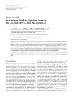
rithm are presented. The system flowchart in Figure 1 gives
an overview of the algorithm. In Section 4, a systematic ex-
perimental evaluation of the performance is described. The
performance is evaluated from two aspects: the blink detec-
tion rate and the tracking accuracy. The blink detection rate
is evaluated using videos collected under varying scenarios,
and the tracking accuracy is evaluated using benchmark data
collected with the Vicon motion capturing system. Section 5
gives some discussion and concludes the paper.
2. DYNAMIC SYSTEMS AND PARTICLE FILT ERS
The fundamental prerequisite of a simultaneous eye tracking
and blink detection system is to accurately recover the dy-
namics of eyes, which can be modeled by a dynamic system.
Open eyes and closed eyes appear to have significantly dif-
ferent appearances. A straightforward way is to model the
dynamics of open-eye and closed-eye individually. We use
two interactive particle filters for this purpose. The poste-
rior probabilities learned by the particle filters are used to
determine which particle filter gives the correct tracks, and
this particle filter is thus labeled as the primary one. Figure 1
gives the diagram of the system. Since the particle filters are
the key part of this blink detection system, in this section,
we present a detailed overview of the dynamic system and its
particle filtering solutions, such that the proposed system for
simultaneous eye tracking and blink detection can be better
understood.
2.1. Dynamic systems

A dynamic system can be described by two mathematical
models. One is the state-transition model, which describes
the system evolution rules, represented by the stochastic pro-
cess
{S
t
}∈R
n
s
×1
(t = 0, 1, ), where
S
t
= F
t

S
t−1
, V
t

. (1)
V
t
∈ R
n
v
×1
is the state transition noise with known proba-
bility density function (PDF) p(V

t
). The other one is the ob-
servation model, which shows the relationship between the
observable measurement of the system and the underlying
hidden state variables. The dynamic system is observed at
discrete times t via realization of the stochastic process, mod-
eled as follows:
Y
t
= H
t

S
t
, W
t

. (2)
Y
t
(t = 0, 1, ) is the discrete observation obtained at time t.
W
t
∈ R
n
w
is the observation noise with known PDF p(W
t
),
which is independent from V

t
. For simplicity, we use capital
letters to refer to the random processes and lowercase letters
to denote the realization of the random processes.
Given that these two system models are known, the prob-
lem is to estimate any function of the state f (S
t
) using the
expectation E[ f (S
t
) | Y
0:t
]. If F
t
and H
t
are linear, and the
two noise PDFs, p(V
t
)andp(W
t
), are Gaussian, the sys-
tem can be characterized by a Kalman filter [13]. Unfortu-
nately, Kalman filters only provide the first-order approxi-
mations for general systems. Extended Kalman Filter (EKF)
[13] is one way to handle the nonlinearity. A more general
J. Wu and M. M. Trivedi 3
Predicting/regenerating the
open-eye particles according
to previous eye tracking

Regenerating/predicting the
closed-eye particles according
to previous eye tracking
Generating initial
particles
One set for open-eye
tracking
One set for closed-eye
tracking
Each particle: consider
a binary classification
Each particle: consider
a binary classification
Tensor PCA for feature
extraction
Tensor PCA for feature
extraction
Open-eye/non-eye: posterior
for open-eye
Use logistic regression
Closed-eye/non-eye: posterior
for closed-eye
Use logistic regression
Posterior: open-eye Posterior: closed-eye
P
open
> P
closed
No
Ye s

Estimation of the open eye
location
Estimation of the closed eye
location
Output of logistic regression:
weight of each particle
Output of logistic regression:
weight of each particle
Figure 1: Flow-chart for eye blink detection system. For every new frame observation, new particles are first predicted from the known
important distribution, and then updated accordingly based on the posterior estimated by logistic regressor in the tensor subspaces. The
best estimation gives the class label (open-eye/closed-eye) as well as the eye location.
framework is provided by particle filtering techniques. Par-
ticle filtering is a Monte Carlo solution for general form dy-
namic systems. As an alternative to the EKF, particle filters
have the advantage that with sufficient samples, the solutions
approach the Bayesian estimate.
2.2. Review of a basic particle filter
Particle filters are sequential analogues of Markov chain
Monte Carlo (MCMC) batch methods. They are also known
as sequential Monte Carlo (SMC) methods. Particle filters
are widely used in positioning, navigation, and tracking for
modeling dynamic systems [14–20]. The basic idea of par-
ticle filtering is to use point mass, or particles, to represent
the probability densities. The tracking problem can be ex-
pressed as a Bayes filtering problem, in which the posterior
distribution of the target state is updated recursively as a new
observation comes in
p

S

t
| Y
0:t

∝ p

Y
t
| S
t
; Y
0:t−1


S
t−1
p

S
t
| S
t−1
; Y
0:t−1

×
p

S
t−1

| Y
0:t−1

dS
t−1
.
(3)
The likelihood p(Y
t
| S
t
; Y
0:t−1
) is the observation model,
and p(S
t
| S
t−1
; Y
0:t−1
) is the state transition model.
There are several versions of the particle filters, such
as sequential importance sampling (SIS) [21, 22]/sampling-
importance resampling (SIR) [22–24], auxiliary particle fil-
ters [22, 25], and Rao-Blackwellized particle filters [20, 22,
26, 27], and so forth. All particle filters are derived based on
the following two assumptions. The first assumption is that
4 EURASIP Journal on Advances in Signal Processing
the state-transition is a first-order Markov process, which
simplifies the state transition model in (3)to

p

S
t
| S
t−1
; Y
0:t−1

=
p

S
t
| S
t−1

. (4)
The second assumption is that the observations Y
1:t
are con-
ditionally independent given known states S
1:t
, which im-
plies that each observation only relies on the current state;
then we have
p

Y
t

| S
t
; Y
0:t−1

=
p

Y
t
| S
t

. (5)
These two assumptions simplify the Bayes filter in (3)to
p

S
t
|Y
0:t

∝
p

Y
t
|S
t



S
t−1
p

S
t
|S
t−1

p

S
t−1
|Y
0:t−1

dS
t−1
.
(6)
Exploiting this, particle filter uses a number of particles
(ω
(i)
, s
(i)
t
) to sequentially compute the expectation of any
function of the state, which is E[ f (S
t

) | y
0:t
], by
E

f

S
t

| y
0:t

=

f

s
t

p

s
t
| y
0:t

ds
t
=


i
ω
(i)
t
f

s
(i)
t

.
(7)
In our work, we use the combination of SIS and SIR.
Equation (6) tells us that the estimation is achieved by a pre-
diction step,

s
t−1
p(s
t
| s
t−1
)p(s
t−1
| y
0:t−1
)ds
t−1
, followed by

an update step, p(y
t
| s
t
). At the prediction step, the new state
s
i
t
is sampled from the state evolution process F
t−1
(s
(i)
t
−1
, ·)to
generate a new cloud of particle filters. With the predicted
state
s
i
t
, an estimate of the observation is obtained, which is
used in the update step to correct the posterior estimate. Each
particle is then reweighted in proportion to the likelihood of
the observation at time t. We adopt the idea of “resampling
when necessary” as suggested by [21, 28, 29], which suggests
that resampling is only necessary when the effective number
of particles is sufficiently low. The SIS/SIR algorithm can be
summarized as in Algorithm 1.
π(s
(i)

t
| s
(i)
0:t
−1
, y
0:t
) = π(s
(i)
t
| s
(i)
t
−1
, y
0:t
) is also called
the proposal distribution. A common and simple choice is to
use the prior distribution [30] as the proposal distribution,
which is also known as a bootstrap filter. We use the boot-
strap filter in our work, and by this way the weight update
can be simplified to
ω
(i)
t
= ω
(i)
t
−1
p


y
t
| s
(i)
t

. (12)
This indicates that the weight update is directly related to the
observational model.
3. PARTICLE FILTERS FOR EYE TRACKING AND
BLINK DETECTION
The appearance of eyes is presented to have significant
changes when blinks occur. To effectively handle such ap-
pearance changes, we use two interactive particle filters, one
for open eyes and the other one for closed eyes. These two
particle filters are only different in the observation measure-
ment. In the following sections, we present the three ele-
ments of the proposed particle filters: state transition model,
observation model, and prediction/update scheme.
(1) For i = 1, , N, draw samples from the importance dis-
tributions (prediction step):
s
(i)
t
∼π

s
t
| s

0:t−1
, y
0:t

;(8)
(2) Evaluate the importance weights for every particle up to a
normalized constant (update step):
ω
(i)
t
= ω
(i)
t−1
p

y
t
| s
(i)
t

p

s
(i)
t
| s
(i)
t
−1


π

s
(i)
t
| s
(i)
0:t−1
, y
0:t

;(9)
(3) Normalize the importance weights:
ω
(i)
t
=

ω
(i)
t

N
j
=1
ω
(j)
t
, i = 1, , N; (10)

(4) Compute an estimate of the effective number of the parti-
cles:
N
eff
=
1

N
i
=1

ω
(i)
t

; (11)
(5) If N
eff
<θ,whereθ is a given threshold, we perform resam-
pling. N particles are drawn from the current particle set
with probabilities proportional to their weights. Replace
the current particle set with this new one, and reset each
new particle’s weight to 1/N.
Algorithm 1: SIS/SIR particle filter.
3.1. State transition model
The system dynamics, which are described by the state vari-
ables, are defined by the location of the eye and the size of
the eye image patches. The state vector is S
t
= (u

t
, v
t
; ρ
t
),
where (u
t
, v
t
) defines the location and ρ
t
is used to define
the size of eye image patches and normalize them to a fixed
size. In other words, the state vector (u
t
, v
t
; ρ
t
) means that the
image patch under study is centered at (u
t
, v
t
) and its size is
40ρ
t
×60ρ
t

,where40×60 is the fixed size of the eye patches
we use in our study.
A second-order autoregressive (AR) model is used for es-
timating the eyes’ movement. The AR model has been widely
used in particle filter tracking literature for modeling the mo-
tion. It can be written as
u
t
= u + A

u
t−1
−u

+ Bµ
t
,
v
t
= v + A

v
t−1
−v

+ Bµ
t
,
(13)
where

u
t
=

u
t
u
t−1

, v
t
=

v
t
v
t−1

. (14)
u and v are the corresponding mean values for u and v.As
pointed out by [31],thisdynamicmodelisactuallyatem-
poral Markov chain. It is capable of capturing complicated
J. Wu and M. M. Trivedi 5
object motion. A and B are matrices representing the deter-
ministic and the stochastic components, respectively. A and
B can be either obtained by a maximum-likelihood estima-
tion or set manually from prior knowledge. µ
t
is the i.i.d.
Gaussian noise.

We use a first-order AR model to model the scale transi-
tion, which is
ρ
t
−ρ = C

ρ
t−1
−ρ

+ Dη
t
. (15)
Similar to the motion model, C is the parameter describing
the system deterministic component, and D is the parameter
describing the system stochastic component.
ρ is the mean
value of the scales, and η
t
is the i.i.d. measurement noise.
We a ssu me η
t
is uniformly distributed. The scale is crucial
for many image appearance-based classifiers. An incorrect
scale causes a significant difference in the image appearance.
Therefore, the scale transition model is one of the most im-
portant prerequisites for obtaining an effective particle fil-
ter for measuring the observation. Experimental evaluation
shows that the AR model with uniform i.i.d. noise is appro-
priate for tracking the scale changes.

3.2. Classification-based observation model
In literature, many efforts have been done to address the
problem of selecting the proposal distribution [15, 32–35]. A
carefully selected proposal distribution can alleviate the sam-
ple depletion problem, which refers to the problem that the
particle-based posterior approximation collapses over time
to a few particles. For example, in [35], AdaBoost is incor-
porated into the proposal distribution to form a mixture
proposal. This is crucial in some typical occlusion scenarios,
since “cross over” targets can be represented by the mixture-
model. However, the introduction of complicated proposal
distributions greatly increases the computational complex-
ity. Also, since blink detection is usually a single-target track-
ing problem, the proposal distribution is more likely to be
single-mode. Therefore, we only use bootstrap particle filter-
ing approach, and avoid the nontrivial proposal distribution
estimation problem.
In this work, we focus on a better observation model
p(y
t
| s
t
). The rationale is based on the observation that
combined with the resampling step, a more accurate likeli-
hood learning from a better observation model can move
the particles to areas of high likelihood. This will in turn
mitigate the sample depletion problem, leading to a signif-
icant increase in performance. In literatures, many existing
approaches use simple online template matching [16, 18,
19, 36] to get the observation model, where the templates

are constructed from low-level features, such as color, edges,
contour, and so forth, from previous observations. The like-
lihood is usually estimated based on a Gaussian distribution
assumption [26, 34]. However, such approaches in a large ex-
tent rely on a reasonably stable feature detection algorithm.
Also, usually a large number of the single low-level feature
points are needed. For example, the contour-based method
requires that the state vector be able to describe the evolution
of all contour points. This results in a high-dimensional state
space. Correspondingly, the computational cost is expensive.
One solution is to use abstracted statistics of these single fea-
ture points, such as using color histogram instead of direct
color measurement. However, this causes a loss in the spatial
layout information, which implies a sacrifice in the localiza-
tion accuracy. Instead we use a subspace-based classification
model for measuring the observation such that a more accu-
rate probability evaluation can be obtained. Statistics learned
from a set of training samples are used for classification in-
stead of simple template matching and online updating. This
can greatly alleviate the problem of error accumulation. The
likelihood estimation problem, p(y
(i)
t
| s
(i)
t
), becomes a prob-
lem of estimating the distribution of a Bernoulli variable,
which is p(y
(i)

t
= 1 | s
(i)
t
). y
(i)
t
= 1 means that the current
state generates a positive example. In our eye tracking and
blink detection problem, it represents that an eye patch is lo-
cated, including both open eye and closed eye. Logistic re-
gression is a straightforward solution for this purpose. Obvi-
ously, other existing classification/regression techniques can
be used as well.
Such classification-based particle filtering framework
makes simultaneous tracking and recognition feasible and
straightforward. There are two different ways to embed the
recognition problem. The first approach is to use a single par-
ticle filter, whose observation model is a multiclass classifier.
Thesecondapproachistousemultipleparticlefilters,where
foreachparticlefilteritsobservationmodelusesabinary
classifier designed for a specific object class. The particle filter
who gets the highest posterior is used to determine the class
label as well as the object location, and at the next frame t+1,
the other particle filters are reinitialized accordingly. We use
the second approach for simultaneous eye tracking and blink
detection. Individual observation models are built for open
eye and closed eye separately, such that two interactive sets
of particles can be obtained. The observation models contain
two parts: tensor subspace analysis for feature extraction, and

logistic regression for class posterior learning. The two parts
are individually discussed in Sections 3.2.1 and 3.2.2.Poste-
rior probabilities measured by particles from these two par-
ticle filters are individually denoted as p
o
= p(y
t
= 1
oe
| s
t
)
and p
c
= p(y
t
= 1
ce
| s
t
), respectively, where y
t
= 1
oe
refers to
the presence of an open eye and y
t
= 1
ce
refers to the presence

of a closed eye.
3.2.1. Subspace analysis for feature extraction
Most existing applications of using particle filters for visual
tracking involve high-dimensional observations. With the in-
crease of the dimensionality in observations, the number of
particles required increases exponentially. Therefore, lower
dimensional feature extraction is necessary. Sparse low-level
features, such as the abstracted statistics of the low-level
features, have been proposed for this purpose. Examples
of the most commonly used features are color histogram
[35, 37], edge density [15, 38], salient points [39], con-
tour points [18, 19], and so forth. The use of such features
makes the system capable of easily accommodating the scale
changes and handling occlusions; however, performance of
6 EURASIP Journal on Advances in Signal Processing
such approaches rely on the robustness of the feature detec-
tion algorithms. For example, color histogram is widely used
for pedestrian and human face tracking; however, its perfor-
mance suffers from the illumination changes. Also, the spa-
tial information and the texture information are discarded,
which may cause the degradation of the localization accu-
racy and in turn deteriorate the performance of the succes-
sive recognition algorithms.
Instead of these variants of low-level features, we use
eigen-subspace for feature extraction and dimensionality re-
duction. Eigenspace projection provides a holistic feature
representation that preserves spatial and textural informa-
tion. It has been widely exploited in computer vision applica-
tions. For example, eigenface has been an effective face recog-
nition technique for decades. Eigenface focuses on finding

the most representative lower-dimensional space in which
the pattern of the input can be best described. It tries to find
a set of “standardized face ingredients” learned from a set of
given face samples. Any face image can be decomposed as the
combination of these standard faces. However, this principal
component analysis- (PCA-) based technique treats each im-
age input as a vector, which causes the ambiguity in image
local structure.
Instead of PCA, in [40], a natural alternative for PCA in
image domain is proposed, which is the multilinear analy-
sis. Multilinear analysis offers a potent mathematical frame-
work for analyzing the multifactor structure of the image en-
semble. For example, a face image ensemble can be analyzed
from the following perspectives: identities, head poses, illu-
mination variations, and facial expressions. Multilinear anal-
ysis uses tensor algebra to tackle the problem of disentangling
these constituent factors. By this way, the sample structures
can be better explored and a more informative data represen-
tation can be achieved. Under different optimization crite-
rion, variants of the multilinear analysis technique have been
proposed. One solution is the direct expansion of the PCA al-
gorithm, TensorPCA from [41], which is obtained under the
criteria of the least reconstruction error. Both PCA and ten-
sorPCA are unsupervised techniques, where the class labels
are not incorporated in such representations. Here we use a
supervised version of the tensor analysis algorithm, which is
called tensor subspace analysis (TSA) [42]. Extended from
locality preservation projections (LPP) [43], TSA detects the
intrinsic geometric structure of the tensor space by learning a
lower-dimensional tensor subspace. We compare both obser-

vation models of using tensorPCA and TSA. TSA preserves
the local structure in the tensor space manifold, hence a bet-
ter performance should be obtained. Experimental evalua-
tion validates this conjecture. In the following paragraphs,
a brief review of the theoretical fundamentals of tensorPCA
and TSA are presented.
PCA is a widely used method for dimensionality reduc-
tion. PCA offers a well-defined model, which aims to find
the subspace that describes the direction of the most vari-
ance and at the same time suppress known noise as well as
possible. Tensor space analysis is used as a natural alterna-
tive for PCA in image domain for efficient computation as
well as avoiding ambiguities in image local spatial structure.
Tensor space analysis handles images using its natural 2D
matrix representation. TensorPCA subspace analysis projects
a high-dimensional rank-2 tensor onto a low-dimensional
rank-2 tensor space, where the tensor subspace projection
minimizes the reconstruction error. Different from the tra-
ditional PCA, tensor space analysis provides techniques for
decomposing the ensemble in order to disentangle the con-
stituent factors or modes. Since the spatial location is deter-
mined by two modes: horizontal position and vertical posi-
tion, tensor space analysis has the ability to preserve the spa-
tial location, while the dimension of the parameter space is
much smaller.
Similarly as the traditional PCA, the tensorPCA projec-
tion finds a set of orthogonal bases that information is best
preserved. Also, tensorPCA subspace projection decreases
the correlation between pixels while the projected coefficient
indicates the information preserved on the corresponding

tensor basis. However, for tensorPCA, the set of bases are
composed by second-order tensors instead of vectors. If we
use matrix X
i
∈ R
M
1
×M
2
to denote the original image sam-
ples, and use matrix Z
i
∈ R
P
1
×P
2
as the tensorPCA projec-
tion result, tensorPCA can be simply computed by [41]
Z
i
=
ˇ
U
T
X
i
ˇ
V. (16)
The column vectors of the left and right projection matrices

ˇ
U and
ˇ
V are the eigenvectors of matrix
S
U
=
N

i=1


X
i
−X
m

X
i
−X
m

T

(17)
and matrix
S
V
=
N


i=1


X
i
−X
m

T

X
i
−X
m


, (18)
respectively; while
X
m
= (1/N)

N
i
=1
X
i
. The dimensionality
of Z

i
reflects the information preserved, which can be con-
trolled by a parameter α. For example, assume the left pro-
jection matrix is computed from S
U
=
ˇ
UC
ˇ
U
T
, then the rank
of the left projection matrix
ˇ
U is determined by
P
1
= arg min
q


q
i
=1
C
i

M
1
i=1

C
i
>α

, (19)
where C
i
is the ith diagonal element of the diagonal eigen-
value matrix C (C
i
>C
j
if i>j). The rank of the right pro-
jection matrix
ˇ
V, P
2
can be decided similarly.
TensorPCA is an unsupervised technique. It is not clear
whether the information preserved is optimal for classifica-
tion. Also, only the Euclidean structure is explored instead of
the possible underlying nonlinear local structure of the man-
ifold. The Laplacian-based dimensionality reduction tech-
nique is an alternate way which focuses on discovering the
nonlinear structure of the manifold [44]. It considers pre-
serving the manifold nature while extracting the subspaces.
By introducing this idea into tensor space analysis, the fol-
lowing objective function can be obtained [42]:
min
U,V


i,j


U
T
X
i
V −U
T
X
j
V


D
i,j
, (20)
J. Wu and M. M. Trivedi 7
where D
i,j
is the weight matrix of a nearest neighbor graph
similar to the one used in LPP [43]:
D
i,j
=
⎧
⎪
⎪
⎪

⎪
⎪
⎨
⎪
⎪
⎪
⎪
⎪
⎩
exp

−

X
i
/


X
i


−
X
j
/


X
j




2
2

if X
i
and X
j
are from the same class,
0ifX
i
and X
j
are from different classes.
(21)
We use the iterative approach provided in [42]tocompute
the left and right projection matrices
ˇ
U and
ˇ
V. The same as
tensorPCA, for a given example X,TSAgives
Z
i
=
ˇ
U
T

X
i
ˇ
V. (22)
At each frame t, the ith particle determines an observa-
tion X
(i)
t
from its state (u
(i)
t
, v
(i)
t
; ρ
(i)
t
). Tensor analysis extracts
the corresponding features Z
(i)
t
. Now the observation model
becomes computing the posterior p(y
(i)
t
= 1 | Z
(i)
t
). For sim-
plicity, in the following section, we omit the time index t and

denote the problem as p(y
(i)
= 1 | Z
(i)
). Logistic regression
is a natural solution for this purpose, which is a generalized
linear model for describing the probability of a Bernoulli dis-
tributed variable.
3.2.2. Logistic regression for modeling probability
Regression is the problem of modeling the conditional ex-
pected value of one random variable based on the obser-
vations of some other random variables, which are usually
referred to as dependent variables. The variable to model
is called the response variable. In the proposed algorithm,
the dependent variables are the coefficients from the ten-
sor subspace projection: Z
(i)
= (z
(i)
1
, , z
(i)
k
, ), and the
response variable to model is the class label y
(i)
, which is a
Bernoulli variable that defines the presence of an eye subject.
For closed-eye particle filter, this Bernoulli variable defines
the presence of a closed eye; while for open-eye particle filter,

this variable defines the presence of an open eye.
The relationship between the class label y
(i)
and its de-
pendent variables, which is the tensor subspace coefficients
(z
(i)
1
, , z
(i)
k
, ) here, can be written as
y
(i)
= g

β
0
+

k
β
k
z
(i)
k

+ e, (23)
where e is the error and g
−1

(•) is called the link function. The
variable y
(i)
can be estimated by
E

y
(i)

=
g

β
0
+

k
β
k
z
(i)
k

. (24)
Logistic regression uses the logit as the link function,
which is logit(p)
= log (p/(1−p)). Therefore, the probability
of the presence of an eye subject can be modeled as
p


y
(i)
= 1 | Z
(i)

=
exp
β
0
+

k
β
k
z
(i)
k
1+exp
β
0
+

k
β
k
z
(i)
k
, (25)
where y

(i)
= 1 means that an eye subject is present.
3.3. State update
The observation models for open eye and closed eye are
individually trained. We have one TSA subspace learned
from open eye/noneye training samples, and another TSA
subspace learned from closed eye/noneye training samples.
Each TSA projection determines a set of transformed fea-
tures, which are denoted as
{Z
(i)
oe
} and {Z
(i)
ce
}. Z
(i)
oe
is the
trans-formed TSA coefficients for the open eyes and Z
(i)
ce
is
the transformed TSA coefficients for the closed eyes. Corre-
spondingly, for open eye and closed eye, individual logistic
regression models are used separately for modeling p
c
and
p
o

as follows:
p
(i)
o
= p
oe

y
(i)
= 1 | Z
(i)
oe

, p
(i)
c
= p
ce

y
(i)
= 1 | Z
(i)
ce

.
(26)
The posteriors are used to update the weights of the corre-
sponding particles, as indicated in (12). The updated weights
are ω

(i)
c
and ω
(i)
o
.
If we have
max
i
p
(i)
o
> max
i
p
(i)
c
, (27)
it indicates the presence of open eyes, and the particle filter
for tracking the open eye is the primary particle filter. Oth-
erwise the eyes of the human subject in the current frame
are closed, which indicates the presence of a blink, and the
particle filter for the closed eye is determined as the primary
particle filter. The use of the max function indicates that our
criteria is to trust the most reliable particle. Other criteria can
also be used, such as the mean or product of the posteriors
from the best K (K>1) particles. The guideline to select the
suitable criteria is that only the good particles, which are the
particles that reliably indicate the presence of eyes, should
be considered. At frame t, assume the particles for the pri-

mary particle filter are
{(u
(i)
t
, v
(i)
t
; ρ
(i)
t
; ω
(i)
t
)}, then the location
(u
t
, v
t
) of the detected eye is determined by
u
t
=

i
ω
(i)
t
u
(i)
t

−1
; v
t
=

i
ω
(i)
t
v
(i)
t
−1
; (28)
and the scale ρ
t
of the eye image patch is
ρ
t
=

i
ω
(i)
t
ρ
(i)
t
−1
. (29)

We compute the effective number of particles N
eff
.If
N
eff
<θ, we perform resampling for the primary particle
filter. The particles with high posteriors are multiplied in
proposition to their posteriors. The secondary particle fil-
ter is reinitialized by setting the particles’ previous states to
(u
t
, v
t
, ρ
t
) and the importance weights ω
(i)
t
to uniform.
4. EXPERIMENTAL EVALUATION
The performance is evaluated from two aspects: the blink de-
tection accuracy and the tracking accuracy. There are two
factors that explain the blink detection rate: first, how many
8 EURASIP Journal on Advances in Signal Processing
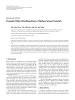
(a) Frame 94 (miss)
Eye close
(b) Frame 379 (c) Frame 392
Eye close
(d) Frame 407 (e) Frame 475
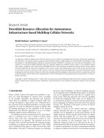
Figure 2: Examples of the blink detection results for indoor videos. Red boxes are tracked eyes, and the blue dots are the center of the eye

locations. The red bar on the top-left indicates the presence of closed eyes.
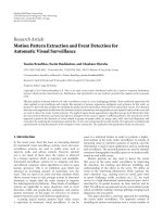
(a) Frame 2
Eye close
(b) Frame 18 (c) Frame 38
Eye close
(d) Frame 45 (false) (e) Frame 135
Figure 3: Examples of the blink detection results for indoor videos. Red boxes are tracked eyes, and the blue dots are the center of the eye
locations. The red bar on the top-left indicates the presence of closed eyes.
blinks are correctly detected; second, the detection accuracy
of the blink duration. Videos collected under different sce-
narios are studied, including indoor videos, in-car videos,
and news report videos. A quantitative comparison is listed.
To evaluate the tracking accuracy, a benchmark data is re-
quired to provide the ground-truth of the eye locations. We
use a marker-based motion capturing system to collect the
ground-truth data. The experimental setup for obtaining the
benchmark data is explained, and the tracking accuracy is
presented. Two hundred particles are used for each parti-
cle filter if not stated otherwise. For training the tensor sub-
spaces and the logistic regression-based posterior estimators,
we use eye samples from FERET gray database to collect
open-eye samples. Closed-eye samples are from these three
sources: (1) FERET database; (2) Cohn-Kanade AU-coded
facial expression database; and (3) online images with closed
eye. Noneye samples are from both the FERET database and
the online images. We have 273 open-eye images; 149 closed-
eye images, and 1879 noneye images. All open-eye, closed-
eye, and noneye samples are resized to 40
×60 for computing
the tensor subspaces and then getting the logistic regressors.

With the information-preservation threshold set as α
= 0.9,
the sizes of the tensorPCA subspaces used for modeling the
open-eye/noneye and closed-eye/noneye samples are 17
×23
and 15
×21, respectively; and the sizes of the TSA subspaces
for open eye/noneye and closed eye/noneye are 18
× 22 and
17
×22, respectively.
4.1. Blink detection accuracy
We use videos collected under different scenarios for evalu-
ating the blink detection accuracy. In the first set of experi-
ments, we use the videos collected from an indoor lab setting.
The subjects are asked to make voluntary long blinks or in-
voluntary short blinks. In the second set of experiments, the
videos collected for drivers in outdoor driving scenarios are
used. In the third set of experiments, we collect videos for
Table 1
No. of
videos
No. of
blinks
No. of correct
detections
No. of false
positives
Indoor
videos

8 133 113 12
In-car
videos
44838 11
News
report
videos
20 456 407 11
Total 32 637 558 34
different archormen/women from news reports. In the sec-
ond and the third experiments, the subjects make natural ac-
tions, such as speaking, so only involuntary short blinks are
present. We have 8 videos from indoor lab settings; 4 videos
of the drivers from an in-car camera; and 20 news report
videos, altogether 637 blinks are present. For in-door videos,
the frame rate is around 25 frames per second, and each vol-
untary blink may last 5-6 frames. For in-car videos, the image
quality is low, and there are significant illumination changes.
Also, the frame rate is fairly low (around 10 frames per sec-
ond). The voluntary blinks may last around 2-3 frames. For
the news report videos, the frame rate is around 15 frames
per second. The videos are compressed and the voluntary
blinks last for about 3-4 frames. In Ta ble 1. the comparison
results are summarized. The true number of blinks, the de-
tected number of blinks, and the number of false positives
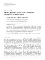
are shown. Images in Figures 2–8 give some examples of the
detection results, which also show the typical video frames
we used for studying. Red boxes show the tracked eye loca-
tion, while blue dots show the center of the tracking results.
If there is a red bar on the top right corner, it means that the

eyes are closed in the current frame. Examples of the typical
false detections or misdetections are also shown.
J. Wu and M. M. Trivedi 9
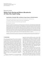
Eye close
(a) Frame 4
Eye close
(b) Frame 35
Eye close
(c) Frame 108 (false) (d) Frame 127
Eye close
(e) Frame 210
Figure 4: Examples of the blink detection results for in-car videos. Red boxes are tracked eyes, and the blue dots are the center of the eye
locations. The red bar on the top-left indicates the presence of closed eyes.
Eye close
(a) Frame 42
Eye close
(b) Frame 302 (false) (c) Frame 349
Eye close
(d) Frame 489
Eye close
(e) Frame 769
Figure 5: Examples of the blink detection results for in-car videos. Red boxes are tracked eyes, and the blue dots are the center of the eye
locations. The red bar on the top-left indicates the presence of closed eyes.
Blink duration time plays an important role in HCI sys-
tems. Involuntary blinks are usually fast while voluntary
blinks usually last longer [45]. Therefore, it is also necessary
to compare the detected blink duration with the manually la-
beled true blink duration (in terms of the frame numbers).
In Figure 9, we show the detected blink duration in compari-
son with the manually labeled blink duration. The horizontal

axis is the blink index, and the vertical axis shows the dura-
tion time in terms of the frame numbers. Experimental eval-
uation shows that the proposed algorithm is capable of cap-
turing short blinks as well as the long voluntary blinks accu-
rately.
As indicated in (27), the ratio of the posterior maxima,
whichis(max
i
p
(i)
o
/max
i
p
(i)
c
), determines the presence of an
open eye or close eye. Figure 10(a) shows an example of
the obtained ratios for one sequence. Log-scale is used. Let
p
o
= max
i
p
(i)
o
and p
c
= max
i

p
(i)
c
, the presence of the closed-
eye frame is determined when p
o
<p
c
, which corresponds
to log (p
o
/p
c
) < 0 in the log-scale. Examples of the corre-
sponding frames are also shown in Figures 10(b)–10(d) for
illustration.
4.2. Comparison of using tensorPCA subspace
and TSA subspace
As stated above, by introducing multilinear analysis, the im-
ages can better preserve the local spatial structure. However,
variants of the tensor subspace basis can be obtained based
on different objective functions. TensorPCA is a straightfor-
ward extension of the 1D PCA analysis. Both are unsuper-
vised approaches. TSA extends LPP that preserves the non-
linear locality in the manifold, which also incorporates the
class information. It is believed that by introducing the lo-
cal manifold structure and the class information, TSA can
obtain a better performance. Experimental evaluations veri-
fied this claim. Particle filters that individually use tensorPCA
subspace and TSA subspace for observation models are com-

pared for eye tracking and blink detection purpose. Examples
of the comparison are shown in Figure 11.Assuggested,TSA
presents a more accurate tracking result. In Figure 11, exam-
ples of the tracking results from both the tensorPCA obser-
vation model and the TSA observation model are shown. In
each subfigure, the left image shows result from the use of
TSA subspace, and the right image shows result from the use
of tensorPCA subspace. Just as above, red bounding boxes
show the tracked eyes, the blue dots show the center of the
detection, and the red bar at the top-right corner indicates
the presence of a detected closed-eye frame. For subspace-
based analysis, image alignment is critical for classification
accuracy. An inaccurate observation model causes errors in
the posterior probability computation, which in turn results
in inaccurate tracking and poor blink detection.
4.3. Comparison of different scale transition models
It is worth noting that for subspace-based observation
model, the scale for normalizing the size of the images is cru-
cial. A bad scale transition model can severely deteriorate the
performance. Two different popular models have been used
to model the scale transition, and the performance is com-
pared. The first one is the AR model as in (15), and the other
one is a Gaussian transition model in which the transition
is controlled by a Gaussian distributed random noise, as fol-
lows:
ρ
t
∼N

ρ

t−1
, σ
2

, (30)
where N (ρ, σ
2
) is a Gaussian distribution with ρ as the mean
and σ
2
as the variance. Examples are shown in Figure 12.
The parameters of the Gaussian transition model is obtained
by the MAP criteria according to a manually labeled train-
ing sequence. In each subfigure, the left image shows the re-
sult from using the AR model for scale transition, and the
10 EURASIP Journal on Advances in Signal Processing
(a) Frame 10 (b) Frame 141 (c) Frame 230
(d) Frame 269 (e) Frame 300
Eye close
(f) Frame 370
Figure 6: Examples of the blink detection results for news report videos. Red boxes are tracked eyes, and the blue dots are the center of the
eye locations. The red bar on the top-left indicates the presence of closed eyes.
Eye close
(a) Frame 10 (b) Frame 100 (c) Frame 129
Eye close
(d) Frame 195
Eye close
(e) Frame 221 (f) Frame 234 (miss)
Figure 7: Examples of the blink detection results for news report videos. Red boxes are tracked eyes, and the blue dots are the center of the
eye locations. The red bar on the top-left indicates the presence of closed eyes.

right one shows the result from using the Gaussian transition
model. Experimental results show that AR model performs
better. It is because AR model has certain “memory” of the
past system dynamics, while Gaussian transition model can
only remember the history of its immediate past. Therefore,
the “short-memory” of Gaussian transition model uses less
information to predict the scale transition trajectory, which
is not effective and in turn causes the failure of the tracking.
4.4. Eye tracking accuracy
Benchmark data is required for evaluating the tracking ac-
curacy. We use the marker-based Vicon motion capture and
analysis system for providing the groundtruth. Vicon system
has both hardware and software components. The hardware
includes a set of infrared cameras (usually at least 4), con-
trolling hardware modules and a host computer to run the
J. Wu and M. M. Trivedi 11
(a) Frame 10
Eye close
(b) Frame 27 (c) Frame 69
(d) Frame 189
Eye close
(e) Frame 192
Eye close
(f) Frame 201
(g) Frame 246 (h) Frame 367
Figure 8: Examples of the blink detection results for news report videos. Red boxes are tracked eyes, and the blue dots are the center of the
eye locations. The red bar on the top-left indicates the presence of closed eyes.
10
5
(a)

25
20
15
10
5
(b)
30
15
(c)
5
(d)
Figure 9: Examples of the duration time of each blink: true blink duration versus detected blink duration. The heights of the bars show the
blink duration (in terms of frame numbers). In each pair of bars, the left (blue) bar shows the duration of the detected blink, and the right
bar (magenta) shows that of the true blink.
12 EURASIP Journal on Advances in Signal Processing
100 200 300 400 500 600
Frame index
6
5
4
3
2
1
0
−1
−2
−3
log(p
o
/p

c
)
Example a
Example b
Example c
(a) Log ratio of the posteriors of being open-eye (p
o
) versus being
closed-eye (p
c
). Red crosses indicate the open-eye frames, and the blue
crosses indicate the detected closed-eye frames
Eye close
Eye close probability
Eye open probability
Example a
00.20.40.60.81
(b)
Eye close
Eye close probability
Eye open probability
Example b
00.20.40.60.81
(c)
Eye close probability
Eye open probability
Example c
00.20.40.60.81
(d)
Figure 10: (a) The log ratio of posteriors log (p

o
/p
c
) for each frame in Seq. 5. (b)–(d) The frames corresponding to examples a, b, and c
in Figure 10(a). The tracked eyes and the posteriors p
c
and p
o
are also shown. In each figure, the top red line shows the posterior of being
closed eye, and the bottom red line shows the posterior of being open eye.
software. The software includes Vicon IQ that manages, sets
up, captures, and processes the motion data, the database
manager for keeping records of the data files, their calibra-
tion files and the models. We use four Vicon MCAM cam-
eras to track four reflective markers. The setup is shown as
in Figure 13. Vicon system tracks the markers’ position in
Vicon’s reference coordinate system, and the video camera
collects the video we need for evaluating the proposed algo-
rithm.
Before collecting data, Vicon system requires prepro-
cesses including camera calibration, data acquisition, and
model building. With the included calibration tool for the
motion capture system, a reflectance marker’s 3D position
can be obtained in either the Vicon camera coordinate system
J. Wu and M. M. Trivedi 13
(a) Frame 17 (b) Frame 100
Eye close
(c) Frame 200
Eye closeEye close
(d) Frame 300

(e) Frame 400
Eye close
(f) Frame 417
Figure 11: Comparison of using TSA subspace versus using tensorPCA subspace in observation models. In each subfigure, the left image
shows the result from using TSA subspace, and the right one shows the result from using tensorPCA subspace.
(a) Frame 100
(b) Frame 200
(c) Frame 380
Figure 12: Comparison of using AR versus using Gaussian tran-
sition model in the scale model. In each subfigure, the left image
shows the result from AR scale transition model, and the right one
shows the result from the Gaussian scale transition model.
or an assigned world coordinate system. Since the Vicon
camera coordinate system is different from the video cam-
era coordinate system, a calibration between these two cam-
era systems is also required. We use a checker-board pattern
with reflectance markers on specified location for this pur-
pose, as shown in Figure 14. Intrinsic parameters KK and
extrinsic parameters R
e
and T
e
are computed. Intrinsic pa-
rameters give the transform from the 3D coordinates in the
camera reference frame to the 2D coordinates in the image
Video camera
Motion capture
system camera
Figure 13: Setup for collecting groundtruth data with Vicon sys-
tem. Cameras in red circles are Vicon infrared cameras, and the

camera in green circle is the video camera for collecting testing se-
quences.
domain, while extrinsic parameters define the transform be-
tween the grid reference frame (as shown in Figure 15)and
the camera reference frame. From intrinsic parameters, the
3D coordinates in the camera coordinate system (X
c
, Y
c
, Z
c
)
T
can be related with the 2D coordinates in the image plane
(x
p
, y
p
)
T
by

x
p
y
p

=
KKφ


X
c
/Z
c
Y
c
/Z
c

, (31)
where φ(
•) is a nonlinear function describing the lens dis-
tortion. Extrinsic parameters describe the relation between
the 3D coordinate in the camera system M
c
= (X
c
, Y
c
, Z
c
)
T
14 EURASIP Journal on Advances in Signal Processing
Marker used by the
motion capturing system
for calibration with the
video system
Checker board used for video camera calibration
Figure 14: Checker board pattern for calibration between video

camera coordinate system and Vicon camera coordinate system. Re-
flectance markers are put at specific locations.
100 200 300 400 500 600
50
100
150
200
250
300
350
400
450
Image points (+) and reprojected grid points (o)
X
O
Z
Y
Figure 15: Example of the grid reference frame.
and the 3D coordinate in a given grid reference frame M
e
=
(X
e
, Y
e
, Z
e
)
T
, as follows:

M
c
= R
e
×M
e
+ T
e
. (32)
Figure 15 gives an example of the grid reference frame.
Each pose of the checker-board defines one grid reference
frame, hence an individual set of extrinsic parameters can
be determined. The reflectance markers are assumed to be
infinitely thin, such that their depth can be neglected. There-
fore, the reflectance markers’ coordinates in current grid ref-
erence frame are known, denoted as M
i
e
. M
i
e
can be trans-
formed back to the video camera reference frame, which
gives the 3D coordinates in the video camera reference frame
M
i
c
, using the corresponding extrinsic parameters R
i
e

and T
i
e
.
These markers are also visible by the Vicon system, as shown
in Figure 16. Calibrated Vicon system gives the 3D positions
of the markers, which are denoted as M
i
v
, in the Vicon cam-
Camera 4 Camera 6
Camera 7 Camera 8
Marker observations
in Vicon system
Figure 16: Reflectance markers observed by Vicon IQ system.
era system reference frame. Hence, M
i
c
and M
i
v
can be related
by an affine transform:
M
i
c
= R
vc
×M
i

v
+ T
vc
. (33)
This relation keeps unchanged when the pose of the check-
board changes. A set of
{(M
i
c
, M
i
e
)} (i = 1, , q)canbeused
to determine this transform. We use the approach proposed
by Goryn and Hein in [49] to estimate R
vc
and T
vc
. The rota-
tion matrix R
vc
can be determined by least-square approach
as follows:
R
vc
= WQ
T
, (34)
where W and Q are unitary matrices obtained from SVD de-
composition of the matrices

c
=
1
N
q

i=1

M
i
c
−M
c

M
i
v
−M
v

T
,
M
c
=
1
q
q

i=1

M
i
c
, M
v
=
1
q
q

i=1
M
i
v
.
(35)
The translation vector T
vc
can be obtained accordingly by
T
vc
= M
c
−R
vc
×M
v
. (36)
Equation (36) together with (31) determines the mapping
from the markers’ 3D position given by Vicon system to the

2D pixel position in the image plane. Therefore, with the Vi-
conIQ system providing the markers’ 3D positions in Vicon
camera systems, we can get our ground-truth data. For reli-
able tracking, four markers are used, as shown in Figure 17.
We use the Vicon system to track the right-eye location as
well as providing the scale of the image, and apply the pro-
posed algorithm on tracking and blink detection of left eye.
After normalization with the scale, the distance between the
right eye and left eye is constant, so that the benchmark data
can be used for evaluating the tracking accuracy. The fixed
size for computing the subspace is 40
×60. We use the center
of the markers as the groundtruth for eyes’ location.
Figure 18 gives an example of the tracking accuracy. The
horizontal axis shows the frame number, and the vertical axis
J. Wu and M. M. Trivedi 15
Reflection markers
Figure 17: Marker deployment for tracking accuracy benchmark
data collection.
0 100 200 300 400 500 600
Frame number
10
5
0
−5
−10
Error (pixel)
Evaluation of tracking accuracy
Figure 18: Tracking error after normalization using the scales. The
horizontal axis is the frame index, and the vertical axis is the track-

ing error in pixels after normalization with the scales.
shows the error in pixels after normalization with the scales.
The error is the distance between the center of detection to
the groundtruth. Experimental results show that in certain
frames, the tracking error is bigger. This is because the pro-
posed algorithm tries to center at the pupil, instead of the
center of the eyes.
5. DISCUSSION AND CONCLUDING REMARKS
A simultaneous eye tracking and blink detection system is
presented in this paper. We used two interactive particle fil-
ters for this purpose, each particle filter serves to track the
eye localization by exploiting AR models for describing the
state transition and a classification-based model in tensor
subspace for measuring the observation. One particle filter
tracks the closed eyes and the other one tracks the open eyes.
The set of particles that gives higher confidence is used to de-
termine the estimated eye location as well as the eye’s status
(open versus closed); also the other set of particles is reini-
tialized accordingly. The system dynamics are described by
two types of hidden state variables: the position and the scale.
We use a second-order autoregression model for describing
the eye’s movement and a first-order autoregression model
for describing the scale transition. Tensor subspace analysis
is used for feature extraction and logistic regression is used
to evaluate the posterior probabilities. The algorithm is eval-
uated using videos collected under different scenarios, in-
cluding both indoor and outdoor data. We evaluated the per-
formance from both the blink detection rate and the track-
ing accuracy perspective. Experimental setup for acquiring
benchmark data to evaluate the accuracy is presented; and

the experimental results are shown, which show that the
proposed algorithm is able to accurately track eye locations
and detect both voluntary long blinks and involuntary short
blinks.
ACKNOWLEDGMENTS
This research was supported in part by grants from the
UC Discovery Program and the Technical Support Working
Group of the US Department of Defense. The authors are
thankful for the assistance and support of their colleagues
from the UCSD Computer Vision and Robotics Research
Laboratory, especially valuable assistance provided by Shinko
Cheng, which made systematic experimental evaluation us-
ing the motion capture system possible.
REFERENCES
[1] N. Kojima, K. Kozuka, T. Nakano, and S. Yamamoto, “De-
tection of consciousness degradation and concentration of a
driver for friendly information service,” in Proceedings of the
IEEE Internat ional Vehicle Electronics Conference, pp. 31–36,
Tottori, Japan, September 2001.
[2] P. Smith, M. Shah, and N. D. V. Lobo, “Monitoring head/eye
motion for driver alertness with one camera,” in Proceedings
of the International Conference on Pattern Recognition, vol. 15,
pp. 636–642, Cambridge, UK, September 2000.
[3] K. Grauman, M. Betke, J. Lombardi, J. Gips, and G. Bradski,
“Communication via eye blinks and eyebrow raises: video-
based human-computer interfaces,” Universal Access in the In-
formation Society, vol. 2, no. 4, pp. 359–373, 2003.
[4] K. Grauman, M. Betke, J. Gips, and G. R. Bradski, “Communi-
cation via eye blinks—detection and duration analysis in real
time,” in Proceedings of the IEEE Computer Society Conference

on Computer Vision and Pattern Recognition, vol. 1, pp. 1010–
1017, Kauai, Hawaii, USA, December 2001.
[5] M. Chau and M. Betke, “Real time eye tracking and blink de-
tection with usb cameras,” Tech. Rep. 2005-12, Boston Univer-
sity Computer Science, Boston, Mass, USA, April 2005.
[6] T. Moriyama, T. Kanade, J. F. Cohn, et al., “Automatic recogni-
tion of eye blinking in spontaneously occurring behavior,” in
Proceedings of the International Conference on Pattern Recogni-
tion (ICPR ’02), vol. 16, pp. 78–81, Kauai, Hawaii, USA, 2002.
[7] D. Gorodnichy, “Second order change detection, and its appli-
cation to blink-controlled perceptual interfaces,” in Proceed-
ings of the International Association of Science and Technol-
og y for Development (IASTED ’03) Conference on Visualization,
Imaging and Image Processing (VIIP ’03), pp. 140–145, Benal-
madena, Spain, September 2001.
[8] T. Morris, P. Blenkhorn, and F. Zaidi, “Blink detection for real-
time eye tracking,” Journal of Network and Computer Applica-
tions, vol. 25, no. 2, pp. 129–143, 2002.
16 EURASIP Journal on Advances in Signal Processing
[9] J. F. Cohn, J. Xiao, T. Moriyama, Z. Ambadar, and T. Kanade,
“Automatic recognition of eye blinking in spontaneously oc-
curring behavior,” 2007, to appear in Behavior Research Meth-
ods, Instruments, and Computers.
[10] J. C. McCall and M. M. Trivedi, “Facial action coding using
multiple visual cues and a hierarchy of particle filters,” in Pro-
ceedings of the IEEE Workshop on Vision for Human Computer
Interaction in Conjunction with IEEE (CVPR ’06), vol. 2006, p.
150, New York, NY, USA, 2006.
[11] J. Wu and M. M. Trivedi, “Robust facial landmark detection
for intelligent vehicle system,” in Proceedings of the IEEE In-

ternational Workshop on Analysis and Modeling of Faces and
Gestures in Conjunction w ith IEEE (ICCV ’05), vol. 3723, pp.
213–228, Beijing, China, 2005.
[12] J. Wu and M. M. Trivedi, “A binary tree for probability learn-
ing in eye detection,” in Proceedings of the IEEE International
Workshop on Face Recognition Grand Challenge in conjunction
with IEEE (CVPR ’05), vol. 3, p. 170, San Diego, Calif, USA,
2005.
[13] G. Welch and G. Bishop, “An introduction to the kalman fil-
ter,” Tech. Rep., University of North Carolina at Chapel Hill,
Chapel Hill, NC, USA, 1995.
[14] F. Gustafsson, F. Gunnarsson, N. Bergman, et al., “Particle fil-
ters for positioning, navigation, and tracking,” IEEE Transac-
tions on Signal Processing, vol. 50, no. 2, pp. 425–437, 2002.
[15] Y. Rui and Y. Chen, “Better proposal distributions: object
tracking using unscented particle filter,” in Proceedings of the
IEEE Computer Society Conference on Computer Vision and
Pattern Recognition (CVPR ’01), vol. 2, pp. 786–793, 2001.
[16] M. Lee, I. Cohen, and S. Jung, “Particle filter with analytical
inference for human body tracking,” in Proceedings of the IEEE
Workshop on Motion and Video Computing, pp. 159–165, De-
cember 2002.
[17] M. Boli
´
c, S. Hong, and P. M. Djuri
´
c, “Performance and com-
plexity analysis of adaptive particle filtering for tracking ap-
plications,” in Conference Record of the Asilomar Conference on
Signals, Systems and Computers, vol. 1, pp. 853–857, 2002.

[18] C. Chang and R. Ansari, “Kernel particle filter: iterative sam-
pling for efficient visual tracking,” in IEEE International Con-
ference on Image Processing, vol. 3, pp. 977–980, 2003.
[19] C. Chang and R. Ansari, “Kernel particle filter for visual track-
ing,” IEEE Signal Processing Letters, vol. 12, no. 3, pp. 242–245,
2005.
[20] A. Giremus, A. Doucet, V. Calmettes, and J Y. Tourneret, “A
rao-blackwellized particle filter for INS/GPS integration,” in
Proceedings of the IEEE International Conference on Acoustics,
Speech and Signal Processing (ICASSP ’04), vol. 3, pp. 964–967,
2004.
[21] J. S. Liu and R. Chen, “Blind deconvolution via sequential
imputation,” Journal of the American Statistical Association,
vol. 90, no. 430, pp. 567–576, 1995.
[22]A.Doucet,deFreitas,J.F.G.,andN.J.Gordon,Sequen-
tial Monte Carlo Methods in Practice,Springer,NewYork,NY,
USA, 2001.
[23] K. Heine, “Unified framework for sampling/importance re-
sampling algorithms,” in Proceedings of the IEEE International
Conference on Information Fusion, vol. 2, pp. 1459–1464, 2005.
[24] J. S. Liu and R. Chen, “Sequential monte carlo methods for dy-
namic systems,” Journal of the American Statistical Association,
vol. 93, no. 443, pp. 1032–1044, 1998.
[25] R. Karlsson, Particle Filtering for Positioning and Tracking Ap-
plications, Ph.D. thesis, Link
¨
oping University, Link
¨
oping, Swe-
den, 2005.

[26]N.J.Gordon,D.J.Salmond,andA.F.M.Smith,“Novel
approach to nonlinear/non-Gaussian Bayesian state estima-
tion,” in IEE Proceedings, Part F: Radar and Signal Processing,
vol. 140, no. 2, pp. 107–113, April 1993.
[27] M. K. Pitt and N. Shephard, “Filtering via simulation: auxil-
iary particle filters,” Journal of the American Statistical Associa-
tion, vol. 94, no. 446, pp. 590–599, 1999.
[28] Z. Khan, T. Batch, and F. Dellaert, “A rao-blackwellized par-
ticle filter for eigen tracking,” in Proceedings of the IEEE
Computer Society Conference on Computer Vision and Pattern
Recognition, vol. 2, pp. 980–986, 2004.
[29] S. Sarkka, A. Vehtari, and J. Lampinen, “Rao-blackwellized
particle filter for multiple target tracking,” Information Fusion,
vol. 8, no. 7, pp. 2–15, 2007.
[30] J. Carpenter, P. Clifford, and P. Fernhead, “An improved parti-
cle filter for non-linear problems,” Tech. Rep., Department of
Statistics, University of Oxford, Oxford, UK, 1997.
[31] A. Doucet, S. Godsill, and C. Andrieu, “On sequential Monte
Carlo sampling methods for Bayesian filtering,” Statistics and
Computing, vol. 10, no. 3, pp. 197–208, 2000.
[32] J. Hol, T. Schon, and F. Gustafsson, “On resampling algorithms
for particle filters,” in Nonlinear Statistical Signal Processing
Workshop, Cambridge, UK, September 2006.
[33] M. Isard and A. Blake, “Visual tracking by stochastic propa-
gation of conditional density,” in Proceedings of the 4th Euro-
pean Conference on Computer Vision (ECCV ’06), pp. 343–356,
Graz, Austria, April 1996.
[34] M. Isard and A. Blake, “Condensation—conditional density
propagation for visual tracking,” International Journal of Com-
puter Vision, vol. 29, no. 1, pp. 5–28, 1998.

[35] K. Nishiyama, “Fast and effective generation of the proposal
distribution for particle filters,” Signal Processing, vol. 85,
no. 12, pp. 2412–2417, 2005.
[36] Y. Guan, R. Fleißner, P. Joyce, and S. M. Krone, “Markov
chainMonteCarloinsmallworlds,”Statistics and Computing,
vol. 16, no. 2, pp. 193–202, 2006.
[37] C.Shen,M.J.Brooks,andA.D.VanHengel,“Augmentedpar-
ticle filtering for efficient visual tracking,” in Proceedings of the
International Conference on Image Processing (ICIP ’05), vol. 3,
pp. 856–859, 2005.
[38] K. Okuma, A. Taleghani, N. De Freitas, J. J. Little, and D.
G. Lowe, “A boosted particle filter: multitarget detection and
tracking,” in Proceedings of the European Conference on Com-
puter Vision, vol. 3021, pp. 28–39, Copenhagen, Denmark,
May 2004.
[39] X. Xu and B. Li, “Head tracking using particle filter with inten-
sity gradient and color histogram,” in Proceedings of the IEEE
International Conference on Multimedia and Expo, (ICME ’05),
vol. 2005, pp. 888–891, 2005.
[40] P. P
´
erez, C. Hue, J. Vermaak, and M. Gangnet, “Color-based
probabilistic tracking,” in Proceedings of the European Confer-
ence on Computer Vision (ECCV ’02), Copenhagen, Denmark,
May 2002.
[41] C. Yang, R. Duraiswami, and L. Davis, “Fast multiple object
tracking via a hierarchical particle filter,” in Proceedings of the
IEEE International Conference on Computer Vision (ICCV ’05),
vol. 1, pp. 212–219, 2005.
[42] M. Pupilli and A. Calway, “Real-time camera tracking using

aparticlefilter,”inProceedings of the British Machine Vision
Conference, pp. 519–528, Oxford Brookes University, Oxford,
UK, September 2005.
J. Wu and M. M. Trivedi 17
[43] M. Alex, O. Vasilescu, and D. Terzopoulos, “Multilinear analy-
sis of image ensembles: Tensorfaces,” in Proceedings of the Eu-
ropean Conference on Computer Vision (ECCV ’02), pp. 447–
460, Copenhagen, Denmark, May 2002.
[44] D. Cai, X. He, and J. Han, “Subspace learning based on ten-
sor analysis,” Tech. Rep. (UIUCDCS-R-2005-2572), Depart-
ment of Computer Science,University of Illinois at Urbana-
Champaign, Champaign, Ill, USA, 2005.
[45] X. He, D. Cai, and P. Niyogi, “Tensor subspace analysis,” in
Proceedings of the Neural Information Processing Systems, 2005.
[46] S. T. Roweis and L. K. Saul, “Nonlinear dimensionality reduc-
tion by locally linear embedding,” Science, vol. 290, no. 5500,
pp. 2323–2326, 2000.
[47] X.He,S.Yan,Y.Hu,P.Niyogi,andH J.Zhang,“Facerecogni-
tion using laplacianfaces,” IEEE Transactions on Pattern Analy-
sis and Machine Intelligence, vol. 27, no. 3, pp. 328–340, 2005.
[48] S. Esaki, Y. Ebisawa, A. Sugioka, and M. Konishi, “Quick menu
selection using eye blink for eye-slaved nonverbal communi-
cator with video-based eye-gaze detection,” in Annual Inter-
national Conference of the IEEE Engineering in Medicine and
Biology, vol. 5, pp. 2322–2325, 1997.
[49] D. Goryn and S. Hein, “On the estimation of rigid body ro-
tation from noisy data,” IEEE Transactions on Pattern Analysis
and Machine Intelligence, vol. 17, no. 12, pp. 1219–1220, 1995.