Báo cáo hóa học: " Research Article Computational Methods for Estimation of Cell Cycle Phase Distributions of Yeast Cells" docx

Hindawi Publishing Corporation
EURASIP Journal on Bioinformatics and Systems Biology
Volume 2007, Article ID 46150, 9 pages
doi:10.1155/2007/46150
Research Article
Computational Methods for Estimation of Cell Cycle Phase
Distributions of Yeast Cells
Antti Niemist
¨
o,
1
Matti Nykter,
1
Tommi Aho,
1
Henna Jalovaara,
2
Kalle Marjanen,
1
Miika Ahdesm
¨
aki,
1
Pekka Ruusuvuori,
1
Mikko Tiainen,
2
Marja-Leena Linne,
1
and Olli Yli-Harja
1

1
Institute of Signal Processing, Tampere University of Technology, P.O. Box 553, 33101 Tampere, Finland
2
MediCel Ltd., Haartmaninkatu 8, 00290 Helsinki, Finland
Received 30 June 2006; Revised 5 March 2007; Accepted 17 June 2007
Recommended by Yidong Chen
Two computational methods for estimating the cell cycle phase distribution of a budding yeast (Saccharomyces cerevisiae) cell
population are presented. The first one is a nonparametric method that is based on the analysis of DNA content in the individual
cells of the population. The DNA content is measured with a fluorescence-activated cell sorter (FACS). The second method is
based on budding index analysis. An automated image analysis method is presented for the task of detecting the cells and buds.
The proposed methods can be used to obtain quantitative information on the cell cycle phase distribution of a budding yeast S.
cerevisiae population. They therefore provide a solid basis for obtaining the complementary information needed in deconvolution
of gene expression data. As a case study, both methods are tested with data that were obtained in a time ser ies experiment with S.
cerevisiae. The details of the time series experiment as well as the image and FACS data obtained in the experiment can be found
in the online additional material at .fi/sgn/csb/yeastdistrib/.
Copyright © 2007 Antti Niemist
¨
o et al. This is an open access article distributed under the Creative Commons Attribution License,
which permits unrestricted use, distribution, and reproduction in any medium, provided the original work is properly cited.
1. INTRODUCTION
Many recent studies have concentrated on the construction
of dynamic models for genetic regulatory networks [1–4]. In
such studies, the gene expression levels of cell-cycle-regulated
genes are observed as time series with a relatively short sam-
pling interval over a relatively long period of time. Because
currentlyitisdifficult to profile single cells, time series mi-
croarray experiments are usually carried out by synchroniz-
ing a population of cells. In a synchronous cell population, all
cells are initially in the same phase of the cell cycle. Regardless
of the synchronization method, synchrony of the cell popu-

lation is lost over time. For the budding yeast Saccharomyces
cerevisiae, cells seem to remain relatively synchronized for
two cell cycles [5], although the loss of synchrony is a con-
tinuous process, and the cells are much less synchronized in
the second cell cycle than in the first cycle.
The unavoidable asynchrony of the cell population re-
sults in that the measured gene expression level is in fact
an average of the true values of the neighboring cell cycle
phases. In the case of a relatively synchronous population,
this effect can be modeled by convolution. Moreover, if the
cell cycle phase distribution of the cell population can be es-
timated, the blurring effect of convolution can be inverted
to obtain an estimate of the true expression level that would
have been obtained in a hypothetical perfectly synchronized
experiment. In the case of the budding yeast, several differ-
ent approaches have been proposed for this task [6, 7]. These
studies have concentrated on the deconvolution task. How-
ever, since the quality of the obtained estimate of the true
expression levels depends on the quality of the estimate of
the cell cycle phase distribution, we concentrate here on the
distribution estimation.
There are two basic approaches to estimating the cell cy-
cle phase distribution of a cell population. In the first one, the
numbers of cells that are in different phases of the cell cycle
are found for one time instant or a short time interval. The
result is an age distribution of the cell population. In the sec-
ond approach, the number of cells that are in a given phase
of the cell cycle is monitored over time. The result is a time
distribution of the cell population. Both types of distribution
estimates can be used for the deconvolution task [6, 7].

A fluorescence-activated cell sorter (FACS) is a device
that can be used to measure the DNA content of a sing le
cell with the aid of fluorescence dyeing. It produces a his-
togram of DNA content in the cells under investigation. In
earlier studies with budding yeast [5, 7, 8], an estimate for
the cell cycle phase distribution of a cell population has b een
2 EURASIP Journal on Bioinformatics and Systems Biology
0
50
100
150
Number of cells
0 200 400 600 800 1000
Amount of DNA
G1
S
G2/M
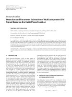
Figure 1: The conventional method for determining the number
of cells in each phase of the cell cycle by using a FACS histogram.
This is an example of an asynchronous cell population; there are
27, 27, and 26 percent of cells in cell cycle phases G1, S, and G2/M,
respectively.
obtained from the FACS histogram by counting the num-
ber of cells in different phases. This has been done manually
by marking the range of each phase in the FACS histogram
and counting the number of cells in that range, see Figure 1.
The results obtained with this approach are dependent on
the method used to determine the location of each phase. It
is also difficult to obtain a good estimate for the S phase of
the cell cycle with this a pproach [9].

The phase of the cell cycle depends by definition on the
amount of DNA in the cell. Cells that are in the G1 phase
have the DNA amount N, whereas cells in the G2/M phase
have the amount 2N. In the S phase, the amount of DNA
is between N and 2N. In this study, we further assume that
the size of a bud of a dividing cell depends on the phase of
the cell cycle [5, 7, 10]. Cells that are in the G1 phase are
assumed not to have a bud, cells that are in the S phase are
assumed to have a small bud, and cells that are in the G2/M
phase are assumed to have a large bud. Based on these as-
sumptions, we propose two computational high-throughput
methods for estimating the cell cycle phase distribution of a
budding yeast cell population. Some preliminary results have
been published in conference proceedings [11, 12].
The first estimation method is a nonparametric method,
in which the estimate of the age distribution is obtained by
analyzing the amount of DNA in the cells with a FACS. The
method has two stages. At the first stage, we use FACS data
from an asynchronous cell population for estimating the rate
of DNA replication in a cell. This estimate can then be used
to find the age distribution of a cell population whose FACS
histogram is known. The population whose distribution is
estimated can be synchronized or it can be otherwise aligned
so that its age distribution is different from a wild-type pop-
ulation. In the second method, the estimate of the time dis-
tribution is obtained by performing budding index analysis
through image analysis. The method is developed for images
taken with a light microscope without any fluorescence stain-
ing, which makes the image analysis significantly more dif-
ficult than if fluorescent micrographs were used [13]. Also,

in contrast to earlier studies where the image analysis is per-
formed manually through visual inspection of the cells [5, 7],
our image analysis method is fully automated.
2. METHODS
In this section, we present two computational methods for
estimation of the cell cycle phase distribution of a yeast
cell population. The FACS-based method is presented in
Section 2.1, and the image analysis methods needed for bud-
ding index analysis are presented in Section 2.2. It should
be noted that neither of the presented methods depends on
the synchronization method. In fact, the methods do not re-
quire the cell population to be synchronized at all. Thus, both
methods can be directly applied to data from any experiment
in which the cell cycle phase dist ribution of the population
differs from that of a wild-type population.
2.1. Distribution estimation using FACS histograms
In a growing cell culture, the number of cells increases. As a
result of cell division, two newborn cells are obtained. Thus,
there are twice as many newborn as dividing cells in the cul-
ture. The age distribution of the wild-type asynchronous cell
population can be modeled as p(t)
= 2
(1−t)
[14]. Here, t
is a discrete variable a nd denotes the cell cycle phase, that
is, the age of the cell from the cell division, normalized to
the interval [0, 1] and uniformly sampled with Δt intervals
as t
∈{0, Δt,2Δt, ,1}. Thus, cells divide at age 1 and
newborn cells are of age 0. This distribution is shown in

Figure 2(a).
Since we know the total number, N, of cells used in the
FACS measurement a s well as the underlying age distribu-
tion p(t), we can compute the number of cells at each small
time interval [t
k
− Δt, t
k
], t
k
∈{Δt,2Δt, ,1} as c(t
k
) =
N(2
(1−(t
k
−Δt))
− 2
(1−t
k
)
). Furthermore, the cumulative num-
ber of cells at time t is C(t)
=

t
i
=0
c(i) = N(2 − 2
(1−t)

). That
is, for a given t, C(t) is the total number of cells at the earlier
phases of the cell cycle.
As we know the cumulative number of cells C(t)andhave
measured the histogram h
a
of the DNA content of the cells
(see Figure 2(b) for a simulated histogram and Figure 1 for
a histogram from a real FACS measurement), we can esti-
mate the DNA replication function, denoted by f (t). This is
a mapping from “number of cells”-“cell cycle phase”-space to
“number of cells”-“amount of DNA”-space, see Figure 2.Itcan
be estimated from the FACS histogram of an asynchronous
population h
a
by finding, for each t ∈{0, Δt,2Δt, ,1},
f (t)
= arg min
K





K

i=0
h
a
(i) − C(t)






,(1)
where h
a
(i) is the value of the FACS histogram of the asyn-
chronous population at the point i,andK
∈ N.
An example of a simulated f (t) is shown in Figure 2(c).
As the FACS histogram h
a
is a discrete measurement of the
Antti Niemist
¨
oetal. 3
0
10
20
30
40
50
60
70
Number of cells
00.20.40.60.81
Cell cycle phase
(a)

0
10
20
30
40
50
60
70
80
×10
2
Number of cells
11.21.41.61.82
Amount of DNA
(b)
1
1.2
1.4
1.6
1.8
2
Amount of DNA
00.20.40.60.81
Cell cycle phase
(c)
Figure 2: A simulated (a) distribution of an asynchronous cell population, (b) noise-free FACS histogram, and (c) DNA replication function.
The details of the data simulation can be found in the online additional material [15].
1
1.2
1.4

1.6
1.8
2
Amount of DNA
00.20.40.60.81
Cell cycle phase
Sim. function
σ
= 0
σ
= 0.001
σ
= 0.01
σ
= 0.03
Figure 3: DNA replication functions estimated from simulated data
with different amounts of noise. Gaussian noise with variance σ is
added to the simulated data as explained in the online additional
material [15].
amount of DNA, the estimated f (t)isadiscreteversionof
the true continuous DNA replication func tion.
Examples of the DNA replication functions estimated
from simulated data under different amounts of noise are
shown in Figure 3 . The effect of the noise is studied by us-
ing a simple additive Gaussian noise model:
x = x + e,(2)
where e ∼ N(0,σ)andx is a noise-free DNA amount of a
cell. T his noise model, although simple, produces FACS his-
tograms that resemble those measured from real data. The
details of the data simulation process can be found in the

online additional material [15]. Figure 3 shows that in the
noise-free case the obtained discrete estimate is consistent
with the underlying DNA replication function f (t). As the
amount of noise increases, the accuracy of the obtained esti-
mate for DNA replication degrades. It would be possible to
improve the quality of the estimate under noisy conditions
by using a model-based estimation approach. However, this
approach would require us to make assumptions about the
form of the true DNA replication function and about the
noise characteristics of FACS measurements. As neither of
these are known in detail, we rely on our proposed nonpara-
metric approach that does not make any assumptions about
the characteristics of the noise or the DNA replication func-
tion.
Having obtained an estimate for the DNA replication
function f (t), we can estimate the age distribution of a syn-
chronous population. We assume that the function f (t)is
the same for all cells, that is, for cells of synchronous as well
as of asynchronous populations. This assumption is justified,
because f (t) represents the DNA replication of a single cell,
and the behavior of a single cell is not thought to be affected
by whether the population is synchronous or asynchronous.
The function f (t) presents the amount of DNA that is
present at each time instant of the cell cycle. Having this in-
formation, we can use the FACS histogram of a synchronous
population to evaluate the number of cells that this amount
of DNA corresponds to. Thus, the age distribution of the cell
population is obtained by
x( t)
=

f (t)

i=0
h
s
(i) −
t−Δt

i=0
x( i), (3)
where f (t) is the value of the DNA replication function
and h
s
(i) is the value from the FACS histogram of the syn-
chronous population at the point i. The obtained age distri-
bution is discrete, and the cell cycle phase parameter t is a
discrete variable, t
∈{0, Δt,2Δt, ,1}.
WhenaFACShistogramfromarealmeasurement(see
Figure 1) is compared with the ideal simulated histogram
(see Figure 2(b)), a significant difference is observed. As dis-
cussed in Section 1, all cells should have an amount of DNA
between N and 2N. Thus, if the histogram indicates cells
4 EURASIP Journal on Bioinformatics and Systems Biology
Figure 4:Thegreencomponentofamicroscopicimageofawild-
type budding yeast cell population. The size of the image is 1388
×
1037 pixels.
having DNA amounts less than N or greater than 2N, the
respective bins can be assumed to be due to measurement er-

rors and should be excluded from the analysis. As illustrated
in Figure 1, the peaks of the histogram correspond to the
G1 (DNA amount N) and G2/M (DNA amount 2N) phases,
while the area between the peaks corresponds to the S phase.
Therefore, all data that are not included in these three areas
should be considered as measurement errors and should be
removed. The removal can be done by estimating the loca-
tions of the two highest peaks and excluding all data that are
not in the range between these two peaks. This preprocessing
step will make the real FACS histogram resemble the ideal
simulated histogram shown in Figure 2(b).
Although the above estimation method was introduced
in the context of a synchronous cell population, it can be ap-
plied to any population of yeast cells. The only requirement
for the applicability of the method is that FACS measure-
ments are available for a wild-type yeast population as well as
for the population whose age distribution is being estimated.
The estimated population can be a synchronized population
or it can be otherwise aligned because of a perturbation.
2.2. Distribution estimation using budding
index analysis
An automated image analysis method for budding index
analysis is needed, because obtaining the budding index data
manually through visual analysis has a number of drawbacks.
One of the drawbacks is that accurate visual analysis is te-
dious and slow, and in a typical exper iment, the number
of budding yeast images for which budding index data are
needed is large. Moreover, manual counting is always subjec-
tive. If visual analysis is perfor med a second time by the same
or a different person, the results will usually not be the same

as they were the first time. With automated image analysis,
objectivit y of the results is guaranteed because the same cri-
teria are always used to determine if a feature in the image
represents a cell or bud, and the results are therefore easily
reproducible.
In budding yeast images, the cell membranes are typical ly
clearly visible as circular or elliptic regions that are darker
than the background. The image shown in Figure 4 is taken
of a wild-type budding yeast population, and is used here in
the presentation of the image analysis methods. Since yeast
cells grow loose in a solution, the scene that is imaged in any
experiment is three-dimensional. Therefore, all the cells are
not visible in the two-dimensional images, because not all of
them are in the same focal plane. Moreover, a bud may be
hidden behind the parent cell. However, to estimate the dis-
tribution of the population, we do not need to know the real
percentage of buds versus parent cells. Rather, it is enough to
find the relative numbers of buds between different images.
Therefore, the goal is to detect cells that are focused relatively
well and to completely ignore cells that are in poor focus.
The first task is segmentation of the images in order
to separate the cell membranes from the background. First,
the effect of uneven illumination is removed from the im-
age with a polynomial fit. After this, the estimates of the
local mean and the local variance are computed. The re-
sulting local mean and variance images are used to form a
two-dimensional histogram. The core of the segm entation
method is the subsequent clustering of the mean-variance
space. The clustering is based on two assumptions. The first
assumption is that the cell membranes are darker than their

neighborhoods on the average. The second assumption is
that if a cell is in focus, it has sharp edges, and the variance
of the cell neighborhood is higher than the variance of the
background of the image.
The result of clustering is a binary image in which the cell
membranes are represented by ones (shown as white pixels)
and the background is represented by zeros (shown as black
pixels). Then, the remaining holes in the cell membranes are
filled by applying the mor phological closing operation with
a circular structuring element inside an 11
× 11 square. Next,
all small objects are removed. The assumption is that objects
that are very small are not cells but result from artifacts in
the original image. The removal is done by labeling the con-
nected components after which it is str aightforward to deter-
mine the sizes of each object and to remove them if necessary.
Finally, the Euclidean distance transform is performed on the
binary image to detect the inner and outer boundaries of the
cell membranes. The result for the image in Figure 4 is shown
in Figure 5.
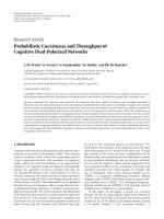
ItcanbeseeninFigure 5 that the inner boundary of
the cell membrane can be used for detection of small buds.
Specifically, in most cases a small bud remains connected
to the parent cell, and there is bridge-like connection be-
tween the parent cell and the bud. A good example is shown
in Figure 6, which shows a part of the image in Figure 4 at
different image processing stages (see below). On the other
hand, the inner boundaries of larger buds are usually discon-
nected from the inner boundar ies of the parent cell. Buds
that are separated from the parent cell in the segmentation

result can thus be detected based on the sizes and numbers
of objects (inner boundaries of a cell membrane) that are in-
side the outer boundary of a cell membrane.
Before any cells or buds are detected, all objects (cell
membranes) that touch the edges of the image are removed
Antti Niemist
¨
oetal. 5
Figure 5: The segmentation result of the image in Figure 4.The
inner and outer boundaries of the cell membranes of the cells are
shown on a black background.
from the image, because it is not realistic to estimate the sizes
of objects that are not completely seen in the image. The next
step is to remove all outer boundaries of the cell membranes.
Since there are now no objects touching the edges of the im-
age, a simple flood-fill can be performed from any pixel at the
edge of the image, after which the outer boundaries can be re-
moved by removing the object that touches the edges of the
image. Some objects that are not in good focus in the orig-
inal image only have a horseshoe-like outer boundary with
no inner boundary, and thus they get removed here, too. One
example of this can be seen near the upper left corner of the
image in Figure 4.
Next, the objects are filled to obtain the image in Figure 7.
This is based on labeling the connected components of the
complement image (black and white reversed). In the labeled
complement image, the component that touches the edges of
the image corresponds to the background, and all the other
components correspond to cell regions that need to be filled
in the original image. The filling is then done according to

the labels of the connected components.
Separation of buds from the parent cells is done with a
modification of the object separation method that has been
proposed in [16]. The method is based on two criteria of the
objects. The first one is a compactness measure:
c
=
4πA
p
2
,(4)
where A is the area of an object and p is the length of its
boundary line, that is, its perimeter. Both of these can be
measured in pixels, but note that c is a dimensionless quan-
tity. The compactness can be computed efficiently using the
chain code representation of objects. Objects that have a low
compactness are candidates for objects that represent cells
that have a small bud. The second criterion is calculated in
the case of bud separation only for objects for which c<0.6.
It is given by
r
= max
x
1
,x
2
∈B
l
b
(x

1
, x
2
)
l
d
(x
1
, x
2
)
,(5)
where x
1
= (x
1
, y
1
)andx
2
= (x
2
, y
2
) are the coordinates
of two points on the boundary of the object, B is the set of
boundary coordinates, l
b
is the distance between the points
along the boundary of the object, and l

d
is the Euclidean dis-
tance between the points. In the case of bud separation, a
cutline is drawn between the corresponding boundary coor-
dinates if r>3.5. The threshold values of c and r were ob-
tained in iterative tests with different threshold values and
different images.
The result of applying the object separation method to
the image of Figure 7 is shown in Figure 8, in which the
buds are marked with the red color. It can be seen that all
small buds are detected and separated from their parent cells.
Moreover, there are no false separations, that is, all cutlines
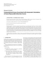
are located between a bud and a parent cell. The steps of the
bud-separation procedure for one cell taken from Figure 4
are illustrated by the images in Figure 6, in which the details
are more clearly visible.
To be able to determine the number of cells that do not
have a bud, the total number of cells must be determined as
well. This number is also used to normalize the numbers of
buds in the budding yeast images. The procedure is similar
to the bud-counting procedure. The main difference is that
the outer boundaries of the cell membranes are utilized in-
stead of the inner boundaries. Because the cells can touch
each other, the object separation method must be applied as
well. Good results can be obtained with c<0.45 and r>3.5
as the criteria in the object separation method.
3. CASE STUDY
The cell cycle phase distribution of a budding yeast p op-
ulation was estimated using the presented methods. The
FACS-based estimation method was used to find the age

distribution, and budding index analysis was used to fi nd
the time distribution. We used alpha factor-based synchro-
nization, which is a block-and-release-type synchroniza-
tion method [17]. The S. cerevisiae strain Y01408 from Eu-
roscarf (BY4741; MATa; his3D1; leu2D0; met15D0; ura3D0;
YIL015w ::kanMX4) was used. Samples of the cultivated pop-
ulation were imaged using a light microscope with the sam-
pling interval of 2 minutes, and samples taken with the sam-
pling interval of 6 minutes were analyzed with a FACS. The
imaging and FACS analysis were performed for a total of 280
minutes. The details of the experiment as well as all the ob-
tained image and FACS data can be found in the online ad-
ditional material [15]. Some of the FACS histograms are also
presented in Figure 9.
The DNA replication function obtained with (1)is
shown in Figure 10. It is interesting to observe that the ob-
tained function is similar to the one that was obtained with
noisy simulated data (σ
= 0.01, see Figure 3). Even though
we removed clear outliers from the data, that is, we removed
the FACS bins beyond the two peaks (as explained above), a
significant amount of measurement noise is still present in
the remaining data. This can be observed from the shape of
the FACS histogram. The peaks, corresponding to the G1 and
G2/Mphases,arewide,andthereisalargenumberofcells
between the peaks. Thus, the proposed estimation method
6 EURASIP Journal on Bioinformatics and Systems Biology
(a) (b) (c) (d)
Figure 6: A part of the image shown in Figure 4 at different image processing stages. The upper left corner is at (x, y) = (609, 383) and the
size of the image is 86

× 105. The image processing stages are (a) original image, (b) segmentation result, (c) result after removing the outer
boundary and filling the remaining inner boundary, and (d) bud-separation result.
Figure 7: The image shown in Figure 5 after removing objects that
touch the edges and filling the objects according to the inner bound-
ary of the cell membrane.
works consistently when applied to the real measurement
data. The obtained replication function suggests that DNA
replication starts at the beginning of the cell cycle a nd contin-
ues in a nearly linear rate throughout the cell cycle. However,
this observation is due to the noise in the data. As demon-
strated earlier by simulation (see Figure 3), additive noise in
FACS measurement biases the estimate towards linear behav-
ior.
The FACS histograms obtained in our experiment sug-
gest that the population was aligned when it was released
from alpha factor arrest. The FACS histograms obtained for
the first few time instants show a clear p eak at the posi-
tion corresponding to the G1 phase (see the online addi-
tional material [15]). This indicates that a majority of the
cells have a DNA amount corresponding to N when the pop-
ulation is released from alpha factor arrest. However, once
the population is released from alpha factor ar rest, the align-
ment is lost rapidly. This behavior can be observed directly
from the FACS histograms, available in the online additional
material.
Figure 8: The image shown in Figure 7 after bud separation. The
two images are similar, but in this image, buds are not connected to
their respective parent cells and are marked with the red color.
Let us now look at some of the estimated distributions.
The age distributions obtained using the FACS-based esti-

mation method are shown in Figure 11. The distributions
have been filtered using a mean filter of length 4 to smooth
out estimation errors. This filter is able to remove estimation
errors caused by numerical problems, but has very little ef-
fect on the shape of the filtered distribution. If we look at
Figure 11(a), we see that the obtained age distribution shows
that a majority of the cells are at an early phase of the cell
cycle and a large number of cells are at the middle part of
the cell cycle. This is consistent with what is observed directly
from the FACS histograms (see Figure 9). Thus, it is clear that
the cells start losing alignment rapidly right after the popula-
tion is released from alpha factor arrest and that cells do not
enter the S phase synchronously at the same time. The esti-
mates presented in Figures 11(b) and 11(c) show that over
time the majority of the cells have moved to a later phase of
the cell cycle, but the alignment is lost even further, which
is illustrated by the fact that the corresponding peaks in the
distributions have spread.
Antti Niemist
¨
oetal. 7
0
50
100
150
200
Number of cells
0 200 400 600 800 1000
Amount of DNA
(a)

0
50
100
150
200
Number of cells
0 200 400 600 800 1000
Amount of DNA
(b)
0
50
100
150
200
Number of cells
0 200 400 600 800 1000
Amount of DNA
(c)
Figure 9: The FACS histograms measured at the time instants: (a) 14 minutes, (b) 44 minutes, and (c) 68 minutes. Corresponding cell cycle
phase distribution estimates are shown in Figure 11.
150
200
250
300
350
Amount of DNA
00.20.40.60.81
Cell cycle phase
Figure 10: The DNA replication function estimated from an asyn-
chronous FACS histogram from the measurement at the time in-

stant 266 minutes. The amount of DNA corresponds to the quan-
tity shown at the x-axis of the FACS histogram; see, for example,
Figure 1.
Automated image analysis was applied to all the images
that were obtained in the time series experiment. For each
image our method determines the total number of cells and
for each cell the size of its bud. The size of the bud is mea-
sured in pixels. The cells were divided into three classes: cells
that do not have a bud, cells that have a small bud (smaller
than one half of the yeast cell), and cells that have a large
bud. These classes are assumed to correspond to the cell cy-
cle phases G1, S, and G2/M, respectively. Because our as-
sumption that the size of a bud depends on the phase of the
cell cycle is an approximation, the respective time distribu-
tions are noisy. The mean filter of length 4 is used to smooth
out this noise. The obtained time distributions are shown
in Figure 12, in which the number of cells in each class at
each time instant is normalized with the number of cells de-
tected at each time instant. The measurement for cells with
no bud in Figure 12(a) is very noisy, and no conclusions can
be made. The measurements for small and large buds in Fig-
ures 12(b) and 12(c) show some alignment: at an early time
instant there are a lot of small buds, and at a later time instant
there are a lot of large buds.
For comparison, the population estimates obtained us-
ing the conventional FACS-based estimation method [7]are
shown in Figure 13. Although the data in the FACS and bud-
counting datasets are noisy, all three estimation methods
show similar alignment in the cell cycle phase distribution of
the cells. The data do not show a high degree of synchroniza-

tion in the way that it should if the population was in perfect
synchrony. However, although a good synchronization is not
observed, different cell cycle phases can still be observed in
the obtained distribution estimates. Thus, due to alpha fac-
tor arrest, cells with equal amounts of DNA have aligned to
some extent.
4. CONCLUSIONS
Two computational methods for estimating the cell cycle
phase distribution of a budding yeast (S. cerevisiae)cellpop-
ulation were presented. The methods are based on the anal-
ysis of the amounts of DNA in the individual cells of a
cell population and on counting the number of buds of a
predefined size in microscopic images. T he method for an-
alyzing the amounts of DNA is a nonparametric method and
does not make any assumptions on DNA replication or the
noise characteristics. The image analysis method is fully au-
tomated, which ensures objectivity of the image processing
results. Neither of the proposed methods makes any assump-
tions on the synchronization method or the synchrony of the
cell population.
The estimated cell cycle phase distributions are discrete
distributions. To be able to utilize the distributions for de-
convolution of gene expression data, continuous distribu-
tions may need to be estimated. For example, an approach
for fitting a normal distribution to a discrete distribution has
been proposed earlier [7]. Existing deconvolution methods
such as the ones published in [6, 7]canbenefitfromourau-
tomated distribution estimation methods.
8 EURASIP Journal on Bioinformatics and Systems Biology
0

50
100
150
200
250
Number of cells
00.20.40.60.81
Cell cycle phase
(a)
0
50
100
150
200
250
Number of cells
00.20.40.60.81
Cell cycle phase
(b)
0
50
100
150
200
250
Number of cells
00.20.40.60.81
Cell cycle phase
(c)
Figure 11: The estimates of the age distributions of the cell population at the time instants (a) 14 minutes, (b) 44 minutes, and (c) 68 minutes

as obtained by the proposed approach. The DNA replication function shown in Figure 10 was used to obtain the distribution estimates.
0
0.2
0.4
0.6
0.8
1
Normalized number of cells
020406080
Time
(a)
0
0.2
0.4
0.6
0.8
1
Normalized number of cells
020406080
Time
(b)
0
0.2
0.4
0.6
0.8
1
Normalized number of cells
020406080
Time

(c)
Figure 12: The estimates of the time distributions of the cell population corresponding to (a) cells with no bud, (b) cells with a small bud,
and (c) cells with a large bud. The number of cells is normalized with the maximum number of cells. Only the first cell cycle data are shown.
Data are not shown for the time instants earlier than 16 minutes because, in the experiment, the microscope was not able to find the correct
focus at these time instants. Note that the axes are different from the axes in Figure 11.
0
0.2
0.4
0.6
0.8
1
Normalized number of cells
10 20 30 40 50 60 70 80 90
Time
(a)
0
0.2
0.4
0.6
0.8
1
Normalized number of cells
10 20 30 40 50 60 70 80 90
Time
(b)
0
0.2
0.4
0.6
0.8

1
Normalized number of cells
10 20 30 40 50 60 70 80 90
Time
(c)
Figure 13: The estimates of the time distributions of the cell population corresponding to the cell cycle phases (a) G1, (b) S, and (c) G2/M as
obtained from FACS histograms. The conventional analysis, illustrated in Figure 1, was used to obtain the time distribution estimates. The
number of cells is normalized with the maximum number of cells. Only the first cell cycle data are shown. Note that the axes are different
from the axes in Figure 11.
ACKNOWLEDGMENTS
The support of the National Technology Agency of Fin-
land (TEKES) and MediCel Ltd. is acknowledged. This work
was also supported by the Academy of Finland (applica-
tion number 213462, Finnish Programme for Centres of Ex-
cellence in Research 2006–2011). The first author is sup-
ported by the Academy of Finland (application number
120325, Researcher Training and Research Abroad). The au-
thors would also like to thank Juha-Pekka Pitk
¨
anen, Ph.D.,
Antti Niemist
¨
oetal. 9
Daniel Nicorici, Ph.D., Jari Niemi, M.S., and Petri Vesanen
for their help in the experiment in which the budding yeast
data that are used in this paper were produced. The first two
authors have contributed equally to this work.
REFERENCES
[1] S. Bornholdt, “Systems biology: less is more in modeling large
genetic networks,” Science, vol. 310, no. 5747, pp. 449–451,

2005.
[2] H. L
¨
ahdesm
¨
aki, I. Shmulevich, and O. Yli-Harja, “On learning
gene regulatory networks under the Boolean network model,”
Machine Learning, vol. 52, no. 1-2, pp. 147–167, 2003.
[3] I. Nachman, A. Regev, and N. Friedman, “Inferring quanti-
tative models of regulatory networks from expression data,”
Bioinformatics, vol. 20, supplement 1, pp. i248–i256, 2004.
[4] J. Tegn
´
er, M. K. S. Yeung, J. Hasty, and J. J. Collins, “Re-
verse engineering gene networks: integrating genetic pertur-
bations with dynamical modeling,” Proceedings of the National
Academy of Sciences of the United States of America, vol. 100,
no. 10, pp. 5944–5949, 2003.
[5] P. T. Spellman, G. Sherlock, M. Q. Zhang, et al., “Comprehen-
sive identification of cell cycle-regulated genes of the yeast sac-
charomyces cerevisiae by microarray hybridization,” Molecular
Biology of the Cell, vol. 9, no. 12, pp. 3273–3297, 1998.
[6] H. L
¨
ahdesm
¨
aki, H. Huttunen, T. Aho, et al., “Estimation and
inversion of the effects of cell population asynchrony in gene
expression time-series,” Signal Processing, vol. 83, no. 4, pp.
835–858, 2003.

[7] Z. Bar-Joseph, S. Farkash, D. K. Gifford, I. Simon, and R.
Rosenfeld, “Deconvolving cell cycle expression data with com-
plementary information,” Bioinformatics, vol. 20, supplement
1, pp. i23–i30, 2004.
[8] M. L. Whitfield, G. Sherlock, A. J. Saldanha, et al., “Identifi-
cation of genes periodically expressed in the human cell cycle
and their expression in tumors,” Molecular Biology of the Cell,
vol. 13, no. 6, pp. 1977–2000, 2002.
[9] A. Lengronne, P. Pasero, A. Bensimon, and E. Schwob, “Mon-
itoring S phase progression globally and locally using BrdU
incorporation in TK
+
yeast strains,” Nucleic Acids Research,
vol. 29, no. 7, pp. 1433–1442, 2001.
[10] T. L. Saito, M. Ohtani, H. Sawai, et al., “SCMD: saccha-
romyces cerevisiae morphological database,” Nucleic Acids Re-
search, vol. 32, Database issue, pp. D319–D322, 2004.
[11] A. Niemist
¨
o, T. Aho, H. Thesleff, et al., “Estimation of popu-
lation effects in synchronized budding yeast experiments,” in
Image Processing: Algorithms and Systems II, vol. 5014 of Pro-
ceedings of SPIE, pp. 448–459, Santa Clara, Calif, USA, January
2003.
[12] A. Niemist
¨
o, M. Nykter, T. Aho, et al., “Distribution estima-
tion of synchronized budding yeast population,” in Proceed-
ings of the Winter International Synposium on Information and
Communication Technologies (WISICT ’04), pp. 243–248, Can-

cun, Mexico, January 2004.
[13] M. Ohtani, A. Saka, F. Sano, Y. Ohya, and S. Morishita, “De-
velopment of image processing program for yeast cell mor-
phology,” Journal of Bioinformatics and Computational Biology,
vol. 1, no. 4, pp. 695–709, 2004.
[14] S. Cooper, “Bacterial growth and division,” in Encyclopedia of
Molecular Cell Biology and Molecular Medicine,R.A.Meyers,
Ed., vol. 1, John Wiley & Sons, New York, NY, USA, 2nd edi-
tion, 2004.
[15] A. Niemist
¨
o, M. Nykter, T. Aho, et al., “Computational
methods for estimation of cell cycle phase distributions of
yeast cells: online supplement,” March 2007, http://www
.cs.tut.fi/sgn/csb/yeastdistrib/.
[16] D. Balthasar, T. Erdmann, J. Pellenz, V. Rehrmann, J. Zep-
pen, and L. Priese, “Real-time detection of arbitrary objects
in alternating industrial environments,” in Proccedings of the
12thScandinavianConferenceonImageAnalysis, pp. 321–328,
Bergen, Norway, June 2001.
[17] B. Futcher, “Cell cycle synchronization,” Methods in Cell Sci-
ence, vol. 21, no. 2-3, pp. 79–86, 1999.