Báo cáo hóa học: " Research Article Inferring Time-Varying Network Topologies from Gene Expression Data" docx

Hindawi Publishing Corporation
EURASIP Journal on Bioinformatics and Systems Biology
Volume 2007, Article ID 51947, 12 pages
doi:10.1155/2007/51947

Research Article
Inferring Time-Varying Network Topologies from
Gene Expression Data
Arvind Rao,1, 2 Alfred O. Hero III,1, 2 David J. States,2, 3 and James Douglas Engel4
1 Department

of Electrical Engineering and Computer Science, University of Michigan, Ann Arbor, MI 48109-2122, USA
Graduate Program, Center for Computational Medicine and Biology, School of Medicine, University of Michigan,
Ann Arbor, MI 48109-2218, USA
3 Department of Human Genetics, School of Medicine, University of Michigan, Ann Arbor, MI 48109-0618, USA
4 Department of Cell and Developmental Biology, School of Medicine, University of Michigan, Ann Arbor, MI 48109-2200, USA
2 Bioinformatics

Received 24 June 2006; Revised 4 December 2006; Accepted 17 February 2007
Recommended by Edward R. Dougherty
Most current methods for gene regulatory network identification lead to the inference of steady-state networks, that is, networks
prevalent over all times, a hypothesis which has been challenged. There has been a need to infer and represent networks in a
dynamic, that is, time-varying fashion, in order to account for different cellular states affecting the interactions amongst genes.
In this work, we present an approach, regime-SSM, to understand gene regulatory networks within such a dynamic setting. The
approach uses a clustering method based on these underlying dynamics, followed by system identification using a state-space
model for each learnt cluster—to infer a network adjacency matrix. We finally indicate our results on the mouse embryonic kidney
dataset as well as the T-cell activation-based expression dataset and demonstrate conformity with reported experimental evidence.
Copyright © 2007 Arvind Rao et al. This is an open access article distributed under the Creative Commons Attribution License,
which permits unrestricted use, distribution, and reproduction in any medium, provided the original work is properly cited.

1.

INTRODUCTION

Most methods of graph inference work very well on stationary time-series data, in that the generating structure for the
time series does not exhibit switching. In [1, 2], some useful method to learn network topologies using linear statespace models (SSM), from T-cell gene expression data, has
been presented. However, it is known that regulatory pathways do not persist over all time. An important recent finding
in which the above is seen to be true is following examination
of regulatory networks during the yeast cell cycle [3], wherein
topologies change depending on underlying (endogeneous
or exogeneous) cell condition. This brings out a need to identify the variation of the “hidden states” regulating gene network topologies and incorporating them into their network
inference framework [4]. This hidden state at time t (denoted
by xt ) might be related to the level of some key metabolite(s)
governing the activity (gt ) of the gene(s). These present a notion of condition specificity which influence the dynamics of
various genes active during that regime (condition). From
time-series microarray data, we aim to partition each gene’s
expression profile into such regimes of expression, during
which the underlying dynamics of the gene’s controlling state

(xt ) can be assumed to be stationary. In [5], the powerful notion of context sensitive boolean networks for gene relationships has been presented. However, at least for short timeseries data, such a boolean characterization of gene state requires a one-bit quantization of the continuous state, which
is difficult without expert biological knowledge of the activation threshold and knowledge of the precise evolution of
gene expression. Here, we work with gene profiles as continuous variables conditioned on the regime of expression. Each
regime is related to the state of a state-space model that is estimated from the data.
Our method (regime-SSM) examines three components:
to find the switch in gene dynamics, we use a change-point
detection (CPD) approach using singular spectrum analysis
(SSA). Following the hypothesis that the mechanism causing the genes to switch at the same time came from a common underlying input [3, 6], we group genes having similar change points. This clustering borrows from a mixture of
Gaussian (MoG) model [7]. The inference of the network adjacency matrix follows from a state-space representation of
expression dynamics among these coclustered genes [1, 2].
Finally, we present analyses on the publicly available embryonic kidney gene expression dataset [8] and the T-cell

2

EURASIP Journal on Bioinformatics and Systems Biology

activation dataset [1], using a combination of the above developed methods and we validate our findings with previously published literature as well as experimental data.
For the embryonic kidney dataset, the biological problem motivating our network inference approach is one of
identifying gene interactions during mammalian nephrogenesis (kidney formation). Nephrogenesis, like several other
developmental processes, involves the precise temporal interaction of several growth factors, differentiation signals, and
transcription factors for the generation and maturation of
progenitor cells. One such key set of transcription factors
is the GATA family, comprising six members, all containing the (–GATA–) binding domain. Among these, Gata2 and
Gata3 have been shown to play a functional role [8, 9] in
nephric development between days 10–12 after fertilization.
From a set of differentially expressed genes pertinent to this
time window (identified from microarray data), our goal is to
prospectively discover regulatory interactions between them
and the Gata2/3 genes. These interactions can then be further
resolved into transcriptional, or signaling interactions on the
basis of additional biological information.
In the T-cell activation dataset, the question is if events
downstream of T-cell activation can be partitioned into early
and late response behaviors, and if so, which genes are active
in a particular phase. Finally, can a network-level influence
be inferred among the genes of each phase and do they correlate with known data? We note here that we are not looking
for the behavior of any particular gene, but only interested in
genes from each phase.
As will be shown in this paper, regime-SSM generates biologically relevant hypotheses regarding time-varying gene
interactions during nephric development and T-cell activation. Several interesting transcripts are seen to be involved in
the process and the influence network hereby generated resolves cyclic dependencies.

The main assumption for the formulation of a linear
state-space model to examine the possibility of gene-gene interactions is that gene expression is a function of the underlying cell state and the expression of other genes at the previous
time step. If longer-range dependencies are to be considered,
the complexity of the model would increase. Another criticism of the model might be that nonlinear interactions cannot be adequately modeled by such a framework. However,
around the equilibrium point (steady state), we can recover a
locally linearized version of this nonlinear behavior.
2.

SSA AND CHANGE-POINT DETECTION

First we introduce some notations. Consider N gene expression profiles, g (1) , g (2) , . . . , g (N) ∈ RT , T being the length of
each gene’s temporal expression profile (as obtained from
microarray expression). The jth time instant of gene i’s expression profile will be denoted by g (i) .
j
State-space partitioning is done using singular spectrum
analysis [10] (SSA). SSA identifies structural change points
in time-series data using a sequential procedure [11]. We will
briefly review this method.

Consider the “windowed” (width NW ) time-series data
(i) (i)
(i)
given by {g1 , g2 , . . . , gNW }, with M (M ≤ NW /2) as some
integer-valued lag parameter, and a replication parameter
K = NW − M + 1. The SSA procedure in CPD involves the
following.
(i) Construction of an l-dimensional subspace: here, a
“trajectory matrix” for the time series, over the interval
[n + 1, n + T] is constructed,
⎛

i,(n)
GB

(i)
gn+1

⎜
⎜ (i)
⎜ gn+2
⎜
=⎜ .
⎜ .
⎜ .
⎝

⎞

(i)
gn+2

(i)
gn+3

(i)
. . . gn+K

(i)
gn+3
.
.

.

(i)
gn+4
.
.
.

(i)
. . . gn+K+1 ⎟
⎟
. ⎟,
..
. ⎟
.
. ⎟
⎠

⎟
⎟

(1)

(i)
(i)
(i)
(i)
gn+M gn+M+1 gn+M+2 . . . gn+NW

where K = NW − M + 1. The columns of the matrix Gi,(n) are

B
(i)
(i)
the vectors Gi,(n) = (gn+ j , . . . , gn+ j+M −1 )T , with j = 1, . . . , K.
j
(ii) Singular vector decomposition of the lag covariance
i,(n)
i,(n)
matrix Ri,n = GB (GB )T yields a collection of singular vectors—a grouping of l of these Singular vectors, corresponding to the l highest eigenvalues—denoted by I =
{1, . . . , l}, establishes a subspace Ln,I of RM .
i,(n)
(iii) Construction of the test matrix: use Gtest defined by
⎛
i,(n)
Gtest

(i)
gn+p+1

⎜
⎜ (i)
⎜ gn+p+2
⎜
=⎜ .
⎜ .
⎜ .
⎝

(i)
gn+p+2

...

(i)
gn+q

(i)
gn+p+3
.
.
.

...
..
.

(i)
gn+q+1
.
.
.

(i)
(i)
(i)
gn+p+M gn+p+M+1 . . . gn+q+M −1

⎞
⎟
⎟

⎟
⎟
⎟.
⎟
⎟
⎠

(2)

Here, we use the length (p) and location (q) of test sample.
We choose p ≥ K, with K = NW − M + 1. Also q > p,
here we take q = p + 1. From this construction, the matrix
columns are the vectors Gi,(n) , j = p + 1, . . . , q. The matrix
j
has dimension M × Q, Q = (q − p) = 1.
(iv) Computation of the detection statistic: the detection
statistics used in the CPD are
(a) the normed Euclidean distance between the column
span of the test matrix, that is, Gi,(n) and the lj
dimensional subspace Ln,I of RM . This is denoted by
Dn,I,p,q ;
(b) the normalized sum of squares of distances, denoted
by Sn = Dn,I,p,q /MQμn,I , with μn,I = Dm,I,0,K , where m
is the largest value of m ≤ n so that the hypothesis of
no change is accepted;
(c) a cumulative sum- (CUSUM-) type statistic W1 = S1 ,
Wn+1 = max{(Wn + Sn+1 − Sn − 1/3MQ), 0}, n ≥ 1.
The CPD procedure declares a structural change in the time
series dynamics if for some time instant n, we observe Wn > h
with the threshold h = (2tα /(MQ)) (1/3)q(3MQ − Q2 + 1),

tα being the (1 − α) quantile of the standard normal distribution.
(v) Choice of algorithm parameters:
(a) window width (NW ): here, we choose NW T/5, T being the length of the original time series, the algorithm


Arvind Rao et al.

3

provides a reliable method of extracting most structural changes. As opposed to choosing a much smaller
NW , this might lead to some outliers being classified as
potential change points, but in our set-up this is preferred in contrast to losing genuine structural changes
based on choosing larger NW ;
(b) choice of lag M: in most cases, choose M = NW /2.
3.

MIXTURE-OF-GAUSSIANS (MoG) CLUSTERING

Having found change points (and thus, regimes) from the
gene trajectories of the differentially expressed genes, our
goal is to now group (cluster) genes with similar temporal
profiles within each regime. In this section, we derive the parameter update equations for a mixture-of-Gaussian clustering paradigm. As will be seen later, the Gaussian assumptions
on the gene expression permit the use of coclustered genes
for the SSM-based network parameter estimation.
We now consider the group of gene expression profiles
G = {g(1) , g(2) , . . . , g(n) }, all of which share a common change
point (time of switch)—c1 . Consider gene profile i, g(i) =
(i) (i)
(i)
[g1 , g2 , . . . , gTc1 ]T , a Tc1 -dimensional random vector which

follows a k-component finite mixture distribution described
by
k

p(g | θ) =

m=1

αm p g | φm ,

(3)

where α1 , . . . , αk are the mixing probabilities, each φm is
the set of parameters defining the mth component, and
θ ≡ {φ1 , . . . , φk , α1 , . . . , αk } is the set of complete parameters
needed to specify the mixture. We have
k

αm ≥ 0,

m = 1, . . . , k,

αm = 1.

(4)

In the E-step of the EM algorithm, the function Q(θ,
θ(t)) ≡ E[log p(G, Z | θ) | G, θ(t)] is computed. This yields
(i)
(i)

wm ≡ E zm | G, θt =

G = g(1) , g(2) , . . . , g(n) ,

(5)

the log-likelihood of a k-component mixture is given by
n

log p(G | θ) = log

p g(i) | θ
i=1

n

=

αm p g

log
i=1

(6)

k
(i)

| φm .

m=1

(i) Treat the labels, Z = {z(1) , . . . , z(n) }, associated with
the n samples—as missing data. Each label is a binary vector
(i)
(i)
(i)
z(i) = [z1 , . . . , zk ], where zm = 1 and z(i) = 0, for p = m inp
(i) was produced by the mth component.
dicate that sample g
In this setting, the expectation maximization algorithm
can be used to derive the cluster parameter (θ) update equations.

,

(7)

(i)
(i)
where wm is the posterior probability of the event zm = 1,
(i)
on observing gm .
The estimate of the number of components (k) is chosen
using a minimum message length (MML) criterion [7]. The
MML criterion borrows from algorithmic information theory and serves to select models of lowest complexity to explain the data. As can be seen below, this complexity has two
components: the first encodes the observed data as a function
of the model and the second encodes the model itself. Hence,
the MML criterion in our setup becomes,

kMML = arg mink − log p G | θ(k) +

k Np + 1
log n ,
2
(8)

N p is number of parameters per component in the k component mixture, given the number of clusters kmin ≤ k ≤ kmax .
In the M-step, for m = 0, 1, . . . , k, θm (t + 1) = arg maxφm
Q(θ, θ(t)), for m : αm (t + 1) > 0, the elements φ’s of the parameter vector estimate θ are typically not closed form and
depend on the specific parametrization of the densities in the
mixture, that is, p(g(i) | φm ). If p(g(i) | φm ) belongs to the
Gaussian density N (μm , Σm ) class, we have, φ = (μ, Σ) and
EM updates yield [7]
αm (t + 1) =
μm (t + 1) =

m=1

For a set of n independently and identically distributed
samples,

αm (t)p g(i) | θm (t)
k
(i)
j =1 α j (t)p g | θ j (t)

Σm (t + 1) =

(i)
n

i=1 wm

n

,

(i) (i)
n
i=1 wm g
(i) ,
n
i=1 wm
(i)
n
i=1 wm

g(i) − μm (t + 1) g(i) − μm (t + 1)
(i)
n
i=1 wm

T

.
(9)

Equations (7) and (9) are the parameter update equations for each of the m = 1, . . . , k cluster components.
For the kidney expression data, since we are interested
in the role of Gata2 and Gata3 during early kidney development, we consider all the genes which have similar change
points as the Gata2 and Gata3 genes, respectively. We perform an MoG clustering within such genes and look at

those coclustered with Gata2 or Gata3. Coclustering within a
regime potentially suggests that the governing dynamics are
the same, even to the extent of coregulation. We note that
just because a gene is coclustered with Gata2 in one regime,
it does not mean that it will cocluster in a different regime.
This approach suggests a way to localize regimes of correlation instead of the traditional global correlation measure that
can mask transient and condition-specific dynamics. For this
gene expression data, the MML penalized criterion indicates
that an adequate number of clusters to describe this data is


4

EURASIP Journal on Bioinformatics and Systems Biology

two (k = 2). In Tables 1 and 2, we indicate some of the genes
with similar coexpression dynamics as Gata2/Gata3 and a
cluster assignment of such genes. We observe that this clustering corresponds to the first phase of embryonic development (days 10–12 dpc), the phase where Gata2 and Gata3 are
perhaps most relevant to kidney development [12–15].
A word about Table 1 is in order. The entries in each column of a row (gene) indicate the change points (as found
by the SSA-CPD procedure) in the time series of the interpolated gene expression profile. Our simulation studies with
the T-cell data indicate that the SSM and CoD performance
is not much worse with the interpolated data compared to
the original time series (Table 7). We note that because of the
present choice of parameters NW , we might have the detection of some false positive change points, but this is preferable to the loss of genuine change points. An examination of
the change points of the various genes in Table 1 indicates
three regimes—between points approximately 1–5, 5–11 and
12–20. The missing entries mean that there was no change
point identified for a certain regime and are thus treated as
such. Since our focus is early Gata3 behavior, we are interested in time points 1–12, and hence we examine the evolution of network-level interactions over the first two regimes

for the genes coclustered in these regimes.
To clarify the validity of the presented approach, we
present a similar analysis on another data set—the T-cell expression data presented in [1]. This data looks at the expression of various genes after T-cell activation using stimulation with phorbolester PMA and ionomycin [16]. This
data has the profiles of about 58 genes over 10 time points
with 44(34 + 10) replicate measurements for each time point.
Since here we have no specific gene in mind (unlike earlier
where we were particularly interested in Gata3 behavior), the
change point procedure (CPD) yields two distinct regimes—
one from time points 1 to 4 and the other from time points 5
to 10. Following the MoG clustering procedure yields the optimal number of clusters to be 1 (from MML) in each regime.
We therefore call these two clusters “early response” and “late
response” genes and then proceed to learn a network relationship amongst them, within each cluster. The CPD and
cluster information for the early and late responses are summarized in Table 3.
4.

STATE-SPACE MODEL

For a given regime, we treat gene expression as an observation related to an underlying hidden cell state (xt ), which is
assumed to govern regime-specific gene expression dynamics for that biological process, globally within the cell. Suppose there are N genes whose expression is related to a single process. The ith gene’s expression vector is denoted as
gt(i) , t = 1, . . . T, where T is the number of time points for
which the data is available. The state-space model (SSM) is
used to model the gene expression (gt(i) , i = 1, 2, . . . , N and
t = 1, 2, . . . , T) as a function of this underlying cell state (xt )
as well as some external inputs. A notion of influence among
genes can be integrated into this model by considering the
SSM inputs to be the gene expression values at the previous

Table 1: Change-point analysis of some key genes, prior to clustering (annotations in Table 8). The numbers indicate the time points
at which regime changes occur for each gene.
Gene symbol Change point I Change point II Change point III

Bmp7
Rara
Pax2
Gata3
Gata2
Gdf11
Npnt
Cd44
Pgf
Pbx1
Ret

6
5
6
5
—
—
—
5
5
5
—

10
11
12
9
—
10

12
11
11
12
10

12
16
15
12
18
20
16
15
—
20
—

Table 2: Some of the genes coclustered with Gata2 and Gata3 after
MoG clustering (annotations in Table 8).
Genes with the same
dynamics as Gata3

Genes with the same
dynamics as Gata2

Bmp7
Nrtn
Pax2
Ros1

Pbx1
Rara
Gdf11

Lamc2
Cldn3
Ros1
Ptprd
Npnt
Cdh16
Cldn4

Table 3: Some of the genes related to early and late responses in
T-cell activation (annotations in Table 9).
Genes related to early response
(time points: 1–4)

Genes related to late response
(time points: 5–10)

CD69
Mcp1
Mcl1
EGR1
JunD
CKR1

CCNA2
CDC2
EGR1

IL2r gamma
IL6
—

time step. The state and observation equations of the statespace model [17] are
(i) state equation:
xt+1 = Axt + Bgt + es,t ; es,t ∼ N (0, Q),
i = 1, . . . , N; t = 1, . . . , T;

(10)

(ii) observation equation:
gt = Cxt + Dgt−1 + eo,t ;

eo,t ∼ N (0, R),

(11)


Arvind Rao et al.

5

Table 4: Assumptions and log-likelihood calculations in the state-space model. The (≡) symbol indicates a definition.
Symbol

Interpretation

Expression

T

Number of time points

—

Rg

Number of replicates

—

P gt | xt

≡

T

e−1/2[gt −Cxt −Dgt−1 ] R

−1 [g −Cx −Dg
t
t
t−1 ]

· (2π)− p/2 det(R)−1/2

t =2
T

P xt | xt−1

e−1/2[xt −Axt−1 −Bgt−1 ] Q

—

−1 [x −Ax
t
t−1 −Bgt−1 ]

· (2π)−k/2 det(Q)−1/2

t =2

P x1

Initial state density assumption

P {x}, {g}

e−1/2[x1 −π1 ] V1 [x1 −π1 ] · (2π)−k/2 det V1

Markov property

Rg

−1/2

T

P x1 (i)
t =2

i=1
Rg

T

−
i=1

T

P xt (i) | xt−1 (i) , gt−1 (i) ·

t =2

P gt (i) | xt (i) , gt−1 (i)
t =1

1 (i)
gt − Cxt (i) − Dgt−1 (i) R−1 gt (i) − Cxt (i) − Dgt−1 (i)
2

−

T
log det(R)
2

T

log P {x}, {g}

Joint log probability

1 (i)
xt − Axt−1 (i) − Bgt−1 (i) Q−1 xt (i) − Axt−1 (i) − Bgt−1 (i)
2
t =1
T −1
1
1
−
log det(Q) − x1 − π1 V1 1 x1 − π1 − log det V1
−
2
2
2
−

−

T(p + k)
log(2π)
2

with xt = [xt(1) , xt(2) , . . . , xt(K) ]T and gt = [gt(1) , gt(2) , . . . ,
gt(N) ]T . A likelihood method [1] is used to estimate the state
dimension K. The noise vectors es,t and eo,t are Gaussian distributed with mean 0 and covariance matrices Q and R, respectively.

From the state and observation equations (10) and (11),
j =1,...,N
we notice that the matrix-valued parameter D = [Di, j ]i=1,...,N
quantifies the influence among genes i and j from one time
instant to the next, within a specific regime. To infer a biological network using D, we use bootstrapping to estimate the
distribution of the strength of association estimates amongst
genes and infer network linkage for those associations that
are observed to be significant.
Within this proposed framework, we segment the overall
gene expression time trajectories into smaller, approximately
stationary, gene expression regimes. We note that the MoG
clustering framework is a nonlinear one in that the regimespecific state space is partitioned into clusters. These cluster
assignments of correlated gene expression vectors can change
with regime, allowing us to capture the sets of genes that interact under changing cell condition.
5.

SYSTEM IDENTIFICATION

We consider the case where we have Rg = B × P realizations of expression data for each gene available. Arguably,

mRNA level is a measure of gene expression, B(= 2) denotes the number of biological replicates, and P(= 16 perfect match probes) denotes the number of probes per gene
transcript. Each of these Rg realizations is T-time-point long
and is obtained from Affymetrix U74Av2 murine microarray raw CEL files. In the section below, we derive the update
equations for maximum-likelihood estimates of the parameters A, B, C, D, Q and R (in (10) and (11)) using an EM
algorithm, based on [17, 18]. The assumptions underlying
this model are outlined in Table 4. A sequence of T output
vectors (g1 , g2 , . . . , gT ) is denoted by {g}, and a subsequence
t
{gt0 , gt0 +1 , . . . , gt1 } by {g}t1 . We treat the (xt , gt ) vector as the
0

complete data and find the log-likelihood log P({x}, {g}) under the above assumptions. The complete E-and M-steps involved in the parameter update steps are outlined in Tables 5
and 6.
6.

BOOTSTRAPPED CONFIDENCE INTERVALS

As suggested above, the entries of the D matrix indicate the
strength of influence among the genes, from one time step to
the next (within each regime). We use bootstrapping to find
confidence intervals for each entry in the D matrix and if it is
significant, we assign a positive or negative direction (+1 or
−1) to this influence.
The bootstrapping procedure [19] is adapted to our situation as follows.


6

EURASIP Journal on Bioinformatics and Systems Biology
Table 5: M-step of the EM algorithm for state-space parameter estimation. The (≡) symbol indicates a definition.

Matrix symbol

Interpretation

Expression

M-Step
π1 new

Initial state mean

x1

new
V1

Initial state covariance

P1 − x1 x1 +
Rg

C new

1
Rg

Rg

x1
Rg

T

i=1 t =1

Rg

Rg

i=1 t =2

i=1 t =1
(i)

i=1 t =1
(i)
Pt,t−1

(i)

− B xt gt−1

−1

T

·

(i)

i=1 t =2
Rg

T

Pt(i)1
−
−1

T

(i)

Rg

T

·

gt−1 (i) gt−1 (i) − gt−1 (i) xt

(i)

i=1 t =1

Input to state matrix

Rg
(i)
Pt,t−1

Rg

Pt(i)

(i) Suppose there are R regimes in the data with change
points (c1 , c2 , . . . , cR ) identified from SSA. For the rth
regime, generate B independent bootstrap samples of
size N (the original number of genes under consideration), -(Y∗ , Y∗ , . . . , Y∗ ) from original data, by random
1

2
B
resampling from g(i) = [gc(i) , . . . , gc(i) ]T .
r
r+1
(ii) Using the EM algorithm for parameter estimation, estimate the value of D (the influence parameter). Denote the estimate of D for the ith bootstrap sample by
Di∗ .
(iii) Compute the sample mean and sample variance of the
estimates of D over all the B bootstrap samples. That
is,
∗

mean = D =
variance =

1

1
B
B

B − 1 i=1

B

Di∗ ,

i=1

(12)

∗

Di − D

∗ 2

.

(iv) Using the above obtained sample mean and variance,
estimate confidence intervals for the elements of D. If
D lies in this bootstrapped confidence interval, we infer
a potential influence and if not, we discard it. Note that

(i)

(i)

xt gt−1 (i) − xt gt−1 (i)

Rg

−1

T

Pt(i)

gt−1 (i) xt (i)

−1

· xt (i) gt−1

(i)

− gt−1 gt−1

(i)

i=1 t =2

1
Rg × (T − 1)

State noise covariance

xt gt−1 (i)

i=1 t =2

i=1 t =2

Qnew

−1

(i)

Pt(i)

−1

T

T

·

−1

T

·
i=1 t =1

T

i=1 t =2

B new

xt gt−1 (i)

i=1 t =1
Rg

Rg

(i)

Pt(i)

i=1 t =1

Input to observation

Pt(i)

(gt (i) gt (i) ) − C new xt gt (i) − Dnew gt−1 (i) gt (i)

gt (i) gt−1 (i) − gt (i) xt
Dnew

−1

T

(i)

Rg

State dynamics matrix

− x1

xt gt−1 (i) ·

T

T

Rg

(i)

i=1 t =1
Rg

1
Rg × T

Output noise covariance

Anew

T

− x1 x1

gt (i) xt − D

Output matrix

Rnew

(i)

i=1

Rg

Rg

T

i=1 t =2

Rg

T

Pt(i) − Anew
i=1 t =2

Pt(i)1,t − B
−

T

gt−1 (i) xt

(i)

i=1 t =2

even though we write D, we carry out this hypothesis
test for each Di, j , i = 1, . . . , n; j = 1, . . . , n; for each of
the n genes under consideration in every regime.

7.

SUMMARY OF ALGORITHM

Within each regime identified by CPD, we model gene expression as Gaussian distributed vectors. We cluster the genes
using a mixture-of-Gaussians (MoG) clustering algorithm [7]
to identify sets of genes which have similar “dynamics of expression” —in that they are correlated within that regime. We
then proceed to learn the dynamic system parameters (matrices A, B, C, D, Q, and R) for the state-space model (SSM)
underlying each of the clusters. We note two important ideas:
(i) we might obtain different cluster assignments for the
genes depending on the regime;
(ii) since all these genes (across clusters within a regime)
are still related to the same biological process, the hidden state xt is shared among these clusters.
Therefore, we learn the SSM parameters in an alternating
manner by updating the estimates from cluster to cluster


Arvind Rao et al.

7

Table 6: E-step of the EM algorithm for state-space parameter estimation.
E-Step
Forward
x1 0

≡

π1

0

V1

≡

V1

xt t−1

Update

Axt−1 t−1 + Bgt−1

Vtt−1

Update

−1
AVtt−1 A + Q

Kt

Update

Vtt−1 C CVtt−1 C + R

xt t

Update

xt t−1 + Kt gt − Cxt t−1 − Dgt−1

Vtt

Update

Vtt−1 − Kt CVtt−1

Backward
T
VT,T −1

Initialization

−1

T −1
I − KT C AVT −1

xt

≡

xt τ

Pt

≡

VtT + xt T xt T

Jt−1

Update

Vtt−1 A Vtt−1

xt−1 T

Update

xt−1 t−1 + Jt−1 x1 T − Axt−1 t−1 − Bgt−2

VtT

Update

−1
Vtt−1 + Jt−1 VtT − Vtt−1 Jt−1

Pt,t−1
VtT 1,t−2
−

≡

Update

−1

T

Vt,t−1 + xt T xt−1 T
−1
T
−1
Vtt−1 Jt−2 + Jt−1 Vt,t−1 − AVtt−1 Jt−2

while still retaining the form of the state vector xt . The learning is done using an expectation-maximization-type algorithm. The number of components during regime-specific
clustering is estimated using a minimum message length criterion. Typically, O(N) iterations suffice to infer the mixture model in each regime with N genes under consideration.
Thus, our proposed approach is as follows.
(i) Identify the N key genes based on required phenotypical characteristic using fold change studies. Preprocess
the gene expression profiles by standardization and cubic spline interpolation.
(ii) Segment each gene’s expression profile into a sequence of state-dependent trajectories (regime change
points), from underlying dynamics, using SSA.
(iii) For each regime (as identified in step 2),
cluster genes using an MoG model so that genes
with correlated expression trajectories cluster together. Learn an SSM [17, 18] for each cluster (from (10) and (11) for estimation of the
mean and covariance matrices of the state vector)
within that regime. The input to observation matrix (D) is indicative of the topology of the network in that regime.
(iv) Examine the network matrices D (by bootstrapping
to find thresholds on strength of influence estimates)
across all regimes to build the time-varying network.

The discussion of the network inference procedure
would be incomplete in the absence of any other algorithms for comparison. For this purpose, we implement the
CoD- (coefficient-of-determination-) based approach [20,
21] along with the models proposed in [1] (SSM) and [22]
(GGM). The CoD method allows us to determine the association between two genes within a regime via an R2 goodness
of fit statistic. The methods of [1, 22] are implemented on the
time-series data (with regard to underlying regime). Such a
study would be useful to determine the relative merits of each

approach. We believe that no one procedure can work for every application and the choice of an appropriate procedure
would be governed by the biological question under investigation. Each of these methods use some underlying assumptions and if these are consistent with the question that we
ask, then that method has great utility. These individual results, their evaluation, and their comparison are summarized
in Section 8.
8.
8.1.

RESULTS
Application to the GATA pathway

To illustrate our approach (regime-SSM), we consider the
embryonic kidney gene expression dataset [8] and study the
set of genes known to have a possible role in early nephric development. An interruption of any gene in this signaling cascade potentially leads to early embryonic lethality or abnormal organ development. An influence network among these
genes would reveal which genes (and their products) become important at a certain phase of nephric development.
The choice of the N(= 47) genes is done using FDR fold
change studies [23] between ureteric bud and metanephric
mesenchyme tissue types, since this spatial tissue expression
is of relevance during early embryonic development. The
dataset is obtained by daily sampling of the mRNA expression ranging from 11.5–16.5 days post coitus (dpc). Detailed
studies of the phenotypes characterizing each of these days is
available from the Mouse Genome Informatics Database at
We follow [24] and use interpolated expression data pre-processing for cluster analysis.
We resample this interpolated profile to obtain twenty points
per gene expression profile. Two key aspects were confirmed
after interpolation [24, 25]: (1) there were no negative expression values introduced, (2) the differences in fold change
were not smoothed out.
Initial experimental studies have suggested that the 10.5–
12.5 dpc are relatively more important in determination of
the course of metanephric development. We chose to explore
which genes (out of the 47 considered) might be relevant in

this specific time window. The SSA-CPD procedure identified several genes which exhibit similar dynamics (have approximately same change points, for any given regime) in the
early phase and distinctly different dynamics in later phases
(Table 1).
Our approach to influence determination using the statespace model yields up to three distinct regimes of expression over all the 47 genes identified from fold change studies
between bud and mesenchyme. MoG clustering followed by


8

EURASIP Journal on Bioinformatics and Systems Biology

Pax2

Mapk1

Lamc2

Acvr2b

Bmp7

Wnt11

Ros1

Gata3

Rara

Gdf11

Kcnj8

Gata3

Pbx1

Mapk1

Pax2

Lamc2

Cd44

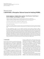
Figure 1: Network topology over regimes (solid lines represent the
first regime, and the dotted lines indicate the second regime).

Acvr2b

Npnt

Lamc2

Gdf11

Cldn7

Kcnj8

Gata3

Npnt

Rara

Figure 3: Steady-state network inferred using CoD (solid lines represent the first regime, and the dotted lines indicate the second
regime).

Rara
CD69

JunD

EGR1

Mcl1

Figure 2: Steady-state network inferred over all time, using [1].
Casp7

state-space modeling yield three regime topologies of which
we are interested in the early regime (days 10.5–12.5). This
influence topology is shown in Figure 1.
We compare our obtained network (using regime-SSM)
with the one obtained using the approach outlined in [1],
shown in Figure 2. We note that the network presented in
Figure 2 extends over all time, that is, days 10.5–16.5 for
which basal influences are represented but transient and
condition-specific influences may be missed. Some of these

transient influences are recaptured in our method (Figure 1)
and are in conformity (lower false positives in network connectivity) with pathway entries in Entrez Gene [15] as well
as in recent reviews on kidney expression [8, 12] (also,
see Table 8). For example, the Mapk1-Rara [26] or the Pax2Gdf11 [27] interactions are completely missed in Figure 2—
this is seen to be the case since these interactions only occur during the 10.5–12.5 dpc regime. We also see that the
Acvr2b-Lamc2 [28] interaction is observed in the steady state
but not in the first regime. This interaction becomes active
in the second regime (first via the Acvr2b-Gdf11 and then via
the Gdf11-Lamc2), indicating that it might not have particular relevance in the day 10.5–12.5 dpc stage. Several of these
predicted interactions need to be experimentally characterized in the laboratory. It is especially interesting to see the
Rara gene in this network, because it is known that Gata3
[29, 30] has tissue-specific expression in some cells of the developing eye. Also Gdf11 exhibits growth factor activity and
is extremely important during organ formation.
In Figure 3, we give the results of the CoD approach of
network inference. Here the Gata3-Pax2 interaction seems
reversed and counterintuitive. As can be seen, some of the
interactions (e.g., Pax2-Gata3) can be seen here (via other
nodes: Mapk1-Wnt11), but there is a need to resolve cycles (Ros1–Wnt11-Mapk1) and feedback/feedforward loops
(Bmp7-Gata3-Wnt11). Both of these topologies can convey
potentially useful information about nephric development.
Thus a potentially useful way to combine these two methods
is to “seed” the network using CoD and then try to resolve
cycles using regime-SSM.

IL6

nFKB

CYP19A1

LAT

Intgam

IL2Rg

CKR1

CDC2

T-cell activation

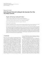
Figure 4: Steady-state network inferred using SSM (solid lines represent the first regime, and the dotted lines indicate the second
regime).

8.2.

T-cell activation

The regime-SSM network is shown in Figure 4. The corresponding network learnt in each regime using CoD is also
shown (Figure 5). The study of this network using GGM
(for the whole time-series data) is already available in [22].
Though there are several interactions of interest discovered
in both the SSM and CoD procedures, we point out a few
of interest. It is already known that synergistic interactions
between IL-6 and IL-1 are involved in T-cell activation [31].
IL-2 receptor transcription is affected by EGR1 [32]. An examination of the topology of these two networks (CoD and
SSM) would indicate some matches and is worth pursuing
for experimental investigation. However, as already alluded
to above, we have to find a way to resolve cycles from the

CoD network [33]. Several of these match the interactions
reported in [1, 22]. However, the additional information that
we can glean is that some of the key interactions occur during
“early response” to stimulation and some occur subsequently
(interleukin-6 mediated T-cell activation) in the “late phase.”
An examination of the gene ontology (GO) terms represented in each cluster as well as the functional annotations
in Entrez Gene shows concordance with literature findings
(Table 9). Because this dataset has been the subject of several
interesting investigations, it would be ideal to ask other questions related to network inference procedures, for the purpose of comparison. One of the primary questions we seek


Arvind Rao et al.

CD69

Mcp1

9

JunD

Pde4b

EGR1

Intgam

Pax2

Mcl1

Mapk1 Cldn4

Fmn

CKR1

Lamc2

Clcn3

Cldn7

Cdh16

Ptprd

Rara

Pbx1

Cd44

Kcnj8

Gdf11
CCNA2

CYP19A1

IL2Rg

CDC2

Figure 6: Steady-state network inferred using GGMs.
Figure 5: Steady-state network inferred using CoD (solid lines represent the first regime, and the dotted lines indicate the second
regime).

to answer is what is the performance of the network inference procedure if a subsampled trajectory is used instead?
In Table 7, the performances of the CoD and SSM algorithms are summarized. Using the T-cell (10 points, 44 replicates) data, we infer a network using the SSM procedure.
With the identified edges as the gold standard for comparison, we now use SSM network inference on an undersampled version of this time series (5 points, 44 replicates) and
check for any new edges ( fnew ) or deletion of edges ( flost ).
Ideally, we would want both these numbers to be zero. fnew
is the fraction of new edges added to the original set and flost
is number of edges lost from the original data network over
both regimes. Further, we now interpolate this undersampled
data to 10 points and carry out network inference. This is
done for each of the identified regimes. The same is done for
the CoD method. We note that this is not a comparison between SSM and CoD (both work with very different assumptions), but of the effect of undersampling the data and subsequently interpolating this undersampled data to the original data length (via resampling). Table 7 suggests that as expected, there is degradation in performance (SSM/CoD) in
the absence of all the available information. However, it is
preferred to infer some false positives rather than lose true
positive edges. This also indicates that interpolated data does
not do worse than the undersampled data in terms of true
positives ( flost ).
We make three observations regarding this method of
network inference.
(i) It is not necessary for the target gene (Gata2/Gata3)
to be present as part of the inferred network. We can
obtain insight into the mechanisms underlying transcription in each regime even if some of the genes with
similar coexpression dynamics as the target gene(s) are

present in the inferred network.
(ii) Probe-level observations from a small number of biological replicates seem to be very informative for network inference. This is because the LDS parameter estimation algorithm uses these multiple expression realizations to iteratively estimate the state mean, covariance and other parameters, notably D [17]. Hence
inspite of few time points, we can use multiple measurements (biological, technical, and probe-level repli-

cates) for reliable network inference. This follows similar observations in [34] that probe-level replicates are
very useful for understanding intergene relationships.
(iii) Following [24], it would seem that several network
hypotheses can individually explain the time evolution behavior captured by the expression data. The
LDS parameter estimation procedure seeks to find a
maximum-likelihood (ML) estimate of the system parameters A, B, C, and D and then finally uses bootstrapping to only infer high confidence interactions.
This ML estimation of the parameters uses an EM algorithm with multiple starts to avoid initializationrelated issues [17], and thus finds the “most consistent” hypothesis which would explain the evolution
of expression data. It is this network hypothesis that
we investigate. Since this network already contains our
gene of interest Gata3, we can proceed to verify these
interactions from literature and experimentally.
9.

DISCUSSION

One of the primary motivations for computational inference
of state specific gene influence networks is the understanding
of transcriptional regulatory mechanisms [36]. The networks
inferred via this approach are fairly general, and thus there is
a need to “decompose” these networks into transcriptional,
signal transduction or metabolic using a combination of biological knowledge and chemical kinetics. Depending on the
insights expected, the tools for dissection of these predicted
influences might vary.
For comparison, we additionally investigated a graphical Gaussian model (GGM) approach as suggested in [35]
using partial correlation as a metric to quantify influence
(Figure 6). This method works for short time-series data but

we could not find a way to incorporate previous expression values as inputs to the evolution of state or individual
observations—something we could explicitly do in the statespace approach. However, we are now in the process of examining the networks inferred by the GGM approach over
the regimes that we have identified from SSA. Again, we observe that the network connections reflect a steady-state behavior and that transient (state-specific) changes in influence
are not fully revealed. The same is observed in the case of
the T-cell data, from the results reported in [22]. A comparison of all the presented methods, along with regime-SSM,
has been presented in Table 10. The comparisons are based


10

EURASIP Journal on Bioinformatics and Systems Biology
Table 7: Functional annotations (Entrez Gene) of some of the genes coclustered with Gata2 and Gata3.

Gene symbol

Gene name

Possible role in nephrogenesis (function)

Bmp7
Rara
Gata2
Gata3
Pax2
Lamc2
Npnt
Ros1
Ptprd
Ret-Gdnf
Gdf11

Mapk1
Kcnj8

Bone morphogenetic protein
Retinoic acid receptor
GATA binding protein 2
GATA binding protein 3
Paired homeobox-2
Laminin
Nephronectin
Ros1 proto-oncogene
protein tyrosine phosphatase
Ret proto-oncogene, Glial neutrophic factor
Growth development factor
Mitogen-activated protein kinase 1
potassium inwardly rectifying channel, subfamily J, member 8

Cell signaling
Retinoic acid pathway, related to eye phenotype
Hematopoiesis, urogenital development
Hematopoiesis, urogenital development
Direct target of Gata2
Cell adhesion molecule
Cell adhesion molecule
Signaling epithelial differentiation
Cell adhesion
Metanephros development
Cell-cell signaling and adhesion
Role in growth factor activity, cell adhesion
Potassium ion transport

Acvr2b

Activin receptor IIB

Transforming growth
factor-beta receptor activity

Table 8: Functional annotations of some of the coclustered genes (early and late responses) following T-cell activation.
Gene symbol

Gene name

Possible role in T-cell activation (function)

CD69
Mcl1
IL6
LAT
EGR1
CDC2
Casp7

CD69 antigen
Myeloid cell leukemia sequence 1 (BCL2-related)
Interleukin 6
Linker for activation of T cells
Early growth response gene 1
Cell division control protein 2
Caspase 7

Early T-cell activation antigen
Mediates cell proliferation and survival
Accessory factor signal
Membrane adapter protein involved in T-cell activation
activates nFKB signaling
Involved in cell-cycle control
Involved in apoptosis

JunD

Jun D proto-oncogene

Regulatory role in T lymphocyte
proliferation and Th cell differentiation

CKR1
CYP19A1
Intgam
nFKB
IL2Rg
Pde4b
Mcp1
CCNA2

Chemokine receptor 1
Cytochrome P450, member 19
Integrin alpha M
nFKB protein
Interleukin-2 receptor gamma

Phosphodiesterase 4B, cAMP-specific
Monocyte chemotactic protein 1
Cyclin A2

negative regulator of the antiviral CD8+ T-cell response
cell proliferation
Mediates phagocytosis-induced apoptosis
Signaling transduction activity
Signaling activity
Mediator of cellular response to extracellular signal
Cytokine gene involved in immunoregulation
Involved in cell-cycle control

Table 9: Results of network inference on original, subsampled, and
interpolated data.
Method (T-cell data)
SSM on original data
SSM on undersampled data
SSM on interpolated data
CoD on original data
CoD on undersampled data
CoD on interpolated data

Edges inferred

fnew

flost

14

—
—
12
—
—

—
3
4
—
3
4

—
3
2
—
2
2

on whether these frameworks permit the inference of directional influences, regime specificity, resolution of cycles, and
modeling of higher lags.
10.

CONCLUSIONS

In this work, we have developed an approach (regime-SSM)
to infer the time-varying nature of gene influence network
topologies, using gene expression data. The proposed approach integrates change-point detection to delineate phases

Arvind Rao et al.

11
Table 10: Comparison of various network inference methods (Y: Yes, N: No).

Method

Direction

Regime-specific

Resolve cycles

Higher lags (> 1)

Nonlinear/locally linear

CoD [20, 21]

Y

Y

N

N

Y

GGM [35]

Y

N

N

N

Y

SSM [1]

Y

N

Y

Y

Y

Regime-SSM

Y

Y

Y

Y

Y

of gene coexpression, MoG clustering implying possible
coregulation, and network inference amongst the regimespecific coclustered genes using a state-space framework. We
can thus incorporate condition specificity of gene expression
dynamics for understanding gene influences. Comparison of
the proposed approach with other current procedures like
GGM or CoD reveals some strengths and would very well
complement existing approaches (Table 10). We believe that
this approach, in conjunction with sequence and transcription factor binding information, can give very valuable clues
to understand the mechanisms of transcriptional regulation
in higher eukaryotes.
ACKNOWLEDGMENTS
The authors gratefully acknowledge the support of the NIH
under Award 5R01-GM028896-21 (JDE). The authors also
thank the three anonymous reviewers for constructive comments to improve this manuscript. The material in this paper
was presented in part at the IEEE International Workshop
on Genomic Signal Processing and Statistics 2005 (GENSIPS05).
REFERENCES
[1] C. Rangel, J. Angus, Z. Ghahramani, et al., “Modeling Tcell activation using gene expression profiling and state-space
models,” Bioinformatics, vol. 20, no. 9, pp. 1361–1372, 2004.
[2] B.-E. Perrin, L. Ralaivola, A. Mazurie, S. Bottani, J. Mallet,
and F. D’Alch´ -Buc, “Gene networks inference using dynamic
e
Bayesian networks,” Bioinformatics, vol. 19, supplement 2, pp.
II138–II148, 2003.

[3] N. M. Luscombe, M. M. Babu, H. Yu, M. Snyder, S. A. Teichmann, and M. Gerstein, “Genomic analysis of regulatory
network dynamics reveals large topological changes,” Nature,
vol. 431, no. 7006, pp. 308–312, 2004.
[4] E. Sontag, A. Kiyatkin, and B. N. Kholodenko, “Inferring dynamic architecture of cellular networks using time series of
gene expression, protein and metabolite data,” Bioinformatics,
vol. 20, no. 12, pp. 1877–1886, 2004.
[5] S. Kim, H. Li, D. Russ, et al., “Context-sensitive probabilistic
Boolean networks to mimic biological regulation,” in Proceedings of Oncogenomics, Phoenix, Ariz, USA, January-February
2003.
[6] H. Li, C. L. Wood, Y. Liu, T. V. Getchell, M. L. Getchell, and A.
J. Stromberg, “Identification of gene expression patterns using
planned linear contrasts,” BMC Bioinformatics, vol. 7, p. 245,
2006.
[7] M. A. T. Figueiredo and A. K. Jain, “Unsupervised learning of
finite mixture models,” IEEE Transactions on Pattern Analysis
and Machine Intelligence, vol. 24, no. 3, pp. 381–396, 2002.

[8] R. O. Stuart, K. T. Bush, and S. K. Nigam, “Changes in gene
expression patterns in the ureteric bud and metanephric mesenchyme in models of kidney development,” Kidney International, vol. 64, no. 6, pp. 1997–2008, 2003.
[9] M. Khandekar, N. Suzuki, J. Lewton, M. Yamamoto, and J.
D. Engel, “Multiple, distant Gata2 enhancers specify temporally and tissue-specific patterning in the developing urogenital system,” Molecular and Cellular Biology, vol. 24, no. 23, pp.
10263–10276, 2004.
[10] N. Golyandina, V. Nekrutkin, and A. Zhigljavsky, Analysis of
Time Series Structure—SSA and Related Techniques, Chapman
& Hall/CRC, New York, NY, USA, 2001.
[11] V. Moskvina and A. Zhigljavsky, “An algorithm based on singular spectrum analysis for change-point detection,” Communications in Statistics Part B: Simulation and Computation,
vol. 32, no. 2, pp. 319–352, 2003.
[12] K. Schwab, L. T. Patterson, B. J. Aronow, R. Luckas, H.-C.
Liang, and S. S. Potter, “A catalogue of gene expression in the
developing kidney,” Kidney International, vol. 64, no. 5, pp.

1588–1604, 2003.
[13] Y. Zhou, K.-C. Lim, K. Onodera, et al., “Rescue of the embryonic lethal hematopoietic defect reveals a critical role
for GATA-2 in urogenital development,” The EMBO Journal,
vol. 17, no. 22, pp. 6689–6700, 1998.
[14] G. A. Challen, G. Martinez, M. J. Davis, et al., “Identifying the
molecular phenotype of renal progenitor cells,” Journal of the
American Society of Nephrology, vol. 15, no. 9, pp. 2344–2357,
2004.
[15] NCBI Pubmed, />fcgi.
[16] H. H. Zadeh, S. Tanavoli, D. D. Haines, and D. L. Kreutzer,
“Despite large-scale T cell activation, only a minor subset of T
cells responding in vitro to Actinobacillus actinomycetemcomitans differentiate into effector T cells,” Journal of Periodontal
Research, vol. 35, no. 3, pp. 127–136, 2000.
[17] Z. Ghahramani and G. E. Hinton, “Parameter estimation for
linear dynamical systems,” Tech. Rep., University of Toronto,
Toronto, Ontario, Canada, 1996.
[18] R. H. Shumway and D. S. Stoffer, Time Series Analysis and Applications, Springer Texts in Statistics, Springer, New York, NY,
USA, 2000.
[19] B. Effron, An Introduction to the Bootstrap, Chapman &
Hall/CRC, New York, NY, USA, 1993.
[20] E. R. Dougherty, S. Kim, and Y. Chen, “Coefficient of determination in nonlinear signal processing,” Signal Processing,
vol. 80, no. 10, pp. 2219–2235, 2000.
[21] S. Kim, E. R. Dougherty, M. L. Bittner, et al., “General nonlinear framework for the analysis of gene interaction via multivariate expression arrays,” Journal of Biomedical Optics, vol. 5,
no. 4, pp. 411–424, 2000.
[22] R. Opgen-Rhein and K. Strimmer, “Using regularized dynamic correlation to infer gene dependency networks from


12

[23]

[24]
[25]

[26]

[27]

[28]

[29]

[30]

[31]

[32]

[33]

[34]

[35]

[36]

EURASIP Journal on Bioinformatics and Systems Biology
time-series microarray data,” in Proceedings of the 4th
International Workshop on Computational Systems Biology
(WCSB ’06), Tampere, Finland, June 2006.

A. O. Hero III, G. Fleury, A. J. Mears, and A. Swaroop, “Multicriteria gene screening for analysis of differential expression
with DNA microarrays,” EURASIP Journal on Applied Signal
Processing, vol. 2004, no. 1, pp. 43–52, 2004, special issue on
genomic signal processing.
Z. Bar-Joseph, “Analyzing time series gene expression data,”
Bioinformatics, vol. 20, no. 16, pp. 2493–2503, 2004.
A. Kundaje, O. Antar, T. Jebara, and C. Leslie, “Learning regulatory networks from sparsely sampled time series expression
data,” Tech. Rep., Columbia University, New York, NY, USA,
2002.
J. E. Balmer and R. Blomhoff, “Gene expression regulation by
retinoic acid,” Journal of Lipid Research, vol. 43, no. 11, pp.
1773–1808, 2002.
A. F. Esquela and S. E.-J. Lee, “Regulation of metanephric kidney development by growth/differentiation factor 11,” Developmental Biology, vol. 257, no. 2, pp. 356–370, 2003.
A. Maeshima, S. Yamashita, K. Maeshima, I. Kojima, and Y.
Nojima, “Activin a produced by ureteric bud is a differentiation factor for metanephric mesenchyme,” Journal of the American Society of Nephrology, vol. 14, no. 6, pp. 1523–1534, 2003.
M. Mori, N. B. Ghyselinck, P. Chambon, and M. Mark, “Systematic immunolocalization of retinoid receptors in developing and adult mouse eyes,” Investigative Ophthalmology and
Visual Science, vol. 42, no. 6, pp. 1312–1318, 2001.
K.-C. Lim, G. Lakshmanan, S. E. Crawford, Y. Gu, F. Grosveld,
and J. D. Engel, “Gata3 loss leads to embryonic lethality due to
noradrenaline deficiency of the sympathetic nervous system,”
Nature Genetics, vol. 25, no. 2, pp. 209–212, 2000.
H. Mizutani, L. T. May, P. B. Sehgal, and T. S. Kupper, “Synergistic interactions of IL-1 and IL-6 in T cell activation. Mitogen but not antigen receptor-induced proliferation of a cloned
T helper cell line is enhanced by exogenous IL-6,” Journal of
Immunology, vol. 143, no. 3, pp. 896–901, 1989.
J.-X. Lin and W. J. Leonard, “The immediate-early gene product Egr-1 regulates the human interleukin- 2 receptor β-chain
promoter through noncanonical Egr and Sp1 binding sites,”
Molecular and Cellular Biology, vol. 17, no. 7, pp. 3714–3722,
1997.
M. J. Herrg˚ rd, M. W. Covert, and B. Ø. Palsson, “Reconcila
ing gene expression data with known genome-scale regulatory network structures,” Genome Research, vol. 13, no. 11, pp.

2423–2434, 2003.
C. Li and W. H. Wong, “Model-based analysis of oligonucleotide arrays: expression index computation and outlier detection,” Proceedings of the National Academy of Sciences of the
United States of America, vol. 98, no. 1, pp. 31–36, 2001.
J. Schă fer and K. Strimmer, An empirical Bayes approach to
a
inferring large-scale gene association networks,” Bioinformatics, vol. 21, no. 6, pp. 754–764, 2005.
A. Rao, A. O. Hero III, D. J. States, and J. D. Engel, “Inference of biologically relevant gene influence networks using the
directed information criterion,” in Proceedings of IEEE International Conference on Acoustics, Speech and Signal Processing
(ICASSP ’06), vol. 2, pp. 1028–1031, Toulouse, France, May
2006.