Báo cáo hóa học: " Research Article Wideband Speech Recovery Using Psychoacoustic Criteria" ppt

Hindawi Publishing Corporation
EURASIP Journal on Audio, Speech, and Music Processing
Volume 2007, Article ID 16816, 18 pages
doi:10.1155/2007/16816
Research Article
Wideband Speech Recovery Using Psychoacoustic Criteria
Visar Berisha and Andreas Spanias
Department of Electrical Engineering, Arizona State University, Tempe, AZ 85287, USA
Received 1 December 2006; Revised 7 March 2007; Accepted 29 June 2007
Recommended by Stephen Voran
Many modern speech bandwidth extension techniques predict the high-frequency band based on features extracted from the lower
band. While this method works for certain types of speech, problems arise when the correlation between the low and the high bands
is not sufficient for adequate prediction. These situations require that additional high-band information is sent to the decoder. This
overhead information, however, can be cleverly quantized using human auditory system models. In this paper, we propose a novel
speech compression method that relies on bandwidth extension. The novelty of the technique lies in an elaborate perceptual model
that determines a quantization scheme for wideband recovery and synthesis. Furthermore, a source/filter bandwidth extension
algorithm based on spectral spline fitting is proposed. Results reveal that the proposed system improves the quality of narrowband
speech while performing at a lower bitrate. When compared to other wideband speech coding schemes, the proposed algorithms
provide comparable speech qualit y at a lower bitrate.
Copyright © 2007 V. Berisha and A. Spanias. This is an open access article distributed under the Creative Commons Attribution
License, which permits unrestricted use, distribution, and reproduction in any medium, provided the original work is properly
cited.
1. INTRODUCTION
The public switched telephony network (PSTN) and most of
today’s cellular networks use speech coders operating with
limited bandwidth (0.3–3.4 kHz), which in turn places a limit
on the naturalness and intelligibility of speech [1]. This is
most problematic for sounds whose energy is spread over the
entire audible spectrum. For example, unvoiced sounds such
as “s” and “f” are often difficult to discriminate with a nar-
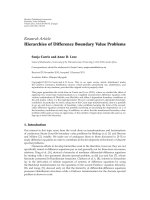
rowband representation. In Figure 1, we provide a plot of the

spectra of a voiced and an unvoiced segment up to 8 kHz.
The energy of the unvoiced segment is spread throughout the
spectrum; however, most of the energy of the voiced segment
lies at the low frequencies. The main goal of algorithms that
aim to recover a wideband (0.3–7 kHz) speech signal from its
narrowband (0.3–3.4 kHz) content is to enhance the intelli-
gibility and the overall quality (pleasantness) of the audio.
Many of these bandwidth extension algorithms make use of
the correlation between the low band a nd the high band in
order to predict the wideband speech signal from extracted
narrowband features [2–5]. Recent studies, however, show
that the mutual information between the narrowband and
the high-frequency bands is insufficient for wideband syn-
thesis solely based on prediction [6–8]. In fact, Nilsson et al.
show that the available narrowband information reduces un-
certainty in the high band, on average, by only
≈10% [8].
As a result, some side information must be transmitted to
the decoder in order to accurately characterize the wide-
band speech. An open question, however, is “how to mini-
mize the amount of side information without affecting syn-
thesized speech quality”? In this paper, we provide a possi-
ble solution through the development of an explicit psychoa-
coustic model that determines a set of perceptually relevant
subbands within the high band. The selected subbands are
coarsely parameterized and sent to the decoder.
Most existing wideband recovery techniques are based on
the source/filter model [2, 4, 5, 9]. These techniques typi-
cally include implicit psychoacoustic principles, such as per-
ceptual weighting filters and dynamic bit allocation schemes

in which lower-frequency components are allotted a larger
number of bits. Although some of these methods were shown
to improve the quality of the coded audio, studies show that
additional coding gain is possible through the integration
of explicit psychoacoustic models [10–13]. Existing psychoa-
coustic models are particularly useful in high-fidelity audio
coding applications; however, their potential has not been
fully utilized in traditional speech compression algorithms
or wideband recovery schemes.
In this paper, we develop a novel psychoacoustic model
for bandwidth extension tasks. The signal is first divided
into subbands. An elaborate loudness estimation model is
used to predict how much a particular frame of audio will
2 EURASIP Journal on Audio, Speech, and Music Processing
012345678
Frequency (kHz)
−40
−20
0
20
Magnitude (dB SPL)
(a)
012345678
Frequency (kHz)
−40
−20
0
20
40
60

Magnitude (dB SPL)
(b)
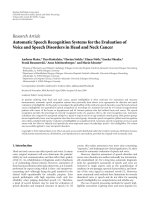
Figure 1: The energy distribution in frequency of an unvoiced
frame (a) and of a voiced frame (b).
benefit from a more precise representation of the high band.
A greedy a lgorithm is proposed that determines the impor-
tance of high-frequency subbands based on perceptual loud-
ness measurements. The model is then used to select and
quantize a subset of subbands within the high band, on a
frame-by-frame basis, for the wideband recovery. A com-
mon method for performing subband ranking in existing au-
dio coding applications is using energy-based metrics [14].
These methods are often inappropriate, however, because en-
ergyaloneisnotasufficient predictor of perceptual impor-
tance. In fact, it is easy to construct scenarios in which a sig-
nal has a smaller energy, yet a larger perceived loudness when
compared to another signal. We provide a solution to this
problem by performing the ranking using an explicit loud-
ness model proposed by Moore et al. in [15].
In addition to the perceptual model, we also propose a
coder/decoder structure in which the lower-frequency band
is encoded using an existing linear predictive coder, w hile
the high band generation is controlled using the perceptual
model. The algorithm is developed such that it can be used as
a “wrapper” around existing narrowband vocoders in order
to improve performance without requiring changes to exist-
ing infrastructure. The underlying bandwidth extension al-
gorithm is based on a source/filter model in which the high-
band envelope and excitation are estimated separately. De-
pending upon the output of the subband ranking algorithm,

the envelope is parameterized at the encoder, and the excita-
tion is predicted from the narrowband excitation. We com-
pare the proposed scheme to one of the modes of the narrow-
band adaptive multirate (AMR) coder and show that the pro-
posed algorithm achieves improved audio quality at a lower
average bitrate [16]. Furthermore, we also compare the pro-
posed scheme to the wideband AMR coder and show com-
parable quality at a lower average bitrate [17].
s
nb
(t)
Frame
classification
Unsample
1/2
Spectral shaping
and gain control
s(t)
s
1,wb
(t)
s
wb
(t)
Figure 2: Bandwidth extension methods based on artificial band
extension and spectral shaping.
The rest of the paper is organized as follows. Section 2
provides a literature review of bandwidth extension algo-
rithms, perceptual models, and their corresponding limita-
tions. Section 3 provides a detailed description of the pro-

posed coder/decoder structure. More specifically, the pro-
posed perceptual model is described in detail, as is the band-
width extension algorithm. In Section 4, we present repre-
sentative objective and subjective comparative results. The
results show the benefits of the perceptual model in the con-
text of bandwidth extension. Section 5 contains concluding
remarks.
2. OVERVIEW OF EXISTING WORK
In this section, we provide an overview of bandwidth ex-
tension algorithms and perceptual models. The specifics of
the most important contributions in both cases are discussed
along with a description of their respective limitations.
2.1. Bandwidth extension
Most bandwidth extension algorithms fall i n one of two cate-
gories, bandwidth extension based on explicit high band gen-
eration and bandwidth extension based on the source/filter
model. Figure 2 shows the block diagram for bandwidth ex-
tension algorithms involving band replication followed by
spectral shaping [18–20]. Consider the narrowband signal
s
nb
(t). To generate an artificial wideband representation, the
signal is first upsampled,
s
1,wb
(t) =
⎧
⎪
⎪
⎨

⎪
⎪
⎩
s
nb

t
2

if mod(t,2)= 0,
0 else.
(1)
This folds the low-band spectrum (0–4 kHz) onto the high
band (4–8 kHz) and fills out the spectrum. Following the
spectr al folding, the high band is transformed by a shaping
filter, s(t),
s
wb
(t) = s
1,wb
(t) ∗ s(t), where ∗ denotes convolution.
(2)
V. Berisha and A. Spanias 3
LP
analysis
s
nb
(t)
a
nb

Feature extraction
Interpolation
Analysis
filter
u
nb
(t)
Excitation
extension
Synthesis
filter
Envelope/gain
predictor
u
wb
(t)
a
wb
σ
+
s
wb
(t)
×
HPF
Figure 3: High-level diagram of tr aditional bandwidth extension techniques based on the source/filter model.
Different shaping filters are typically used for different frame
types. For example, the shaping associated with a voiced
frame may introduce a pronounced spectr a l tilt, whereas the
shaping of an unvoiced frame tends to maintain a flat spec-

trum. In addition to the high band shaping, a gain control
mechanism controls the gains of the low band and the high
band such that their relative levels are suitable.
Examples of techniques based on similar principles in-
clude [18–20]. Although these simple techniques can po-
tentially improve the quality of the speech, audible artifacts
are often induced. Therefore, more sophisticated techniques
based on the source/filter model have been developed.
Most successful bandwidth extension algorithms are
based on the source/filter speech production model [2–
5, 21]. The autoregressive (AR) model for speech synthesis
is given by
s
nb
(t) = u
nb
(t) ∗

h
nb
(t), (3)
where

h
nb
(t) is the impulse response of the all-pole filter
given by

H
nb

(z) = σ/

A
nb
(z).

A
nb
(z)isaquantizedversion
of the Nth order linear prediction (LP) filter given by
A
nb
(z) = 1 −
N

i=1
a
i,nb
z
−i
,(4)
σ is a scalar gain factor, and
u
nb
(t) is a quantized version of
u
nb
(t) = s
nb
(t) −

N

i=1
a
i,nb
s
nb
(t − i). (5)
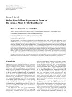
A general procedure for performing wideband recovery
based on the speech production model is given in Figure 3
[21]. In general, a two-step process is taken to recover the
missing band. The first step involves the estimation of the
wideband source-filter parameters, a
wb
,givencertainfea-
tures extracted from the narrowband speech signal, s
nb
(t).
The second step involves extending the narrowband excita-
tion, u
nb
(t). The estimated parameters are then used to syn-
thesize the wideband speech estimate. The resulting speech is
high-pass filtered and added to a 16 kHz resampled version of
the orig inal narrowband speech, denoted by s

nb
(t), given by
s
wb

(t) = s

nb
(t)+σg
HPF
(t) ∗

h
wb
(t) ∗ u
wb
(t)

,(6)
where g
HPF
(t) is the high-pass filter that restricts the synthe-
sized signal within the missing band prior to the addition
with the original narrowband signal. This approach has been
successful in a number of different algorithms [4, 21–27]. In
[22, 23], the authors make use of dual, coupled codebooks
for parameter estimation. In [4, 24, 25], the authors use sta-
tistical recovery functions that are obtained from pretrained
Gaussian mixture models (GMMs) in conjunction with hid-
den Markov models (HMMs). Yet another set of techniques
use linear wideband recovery functions [26, 27].
The underlying assumption for most of these approaches
is that there is sufficient correlation or statistical dependency
between the narrowband features and the wideband envelope
to be predicted. While this is true for some frames, it has been

shown that the assumption does not hold in general [6–8].
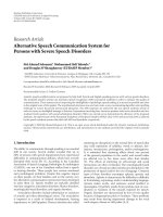
In Figure 4, we show examples of two frames that illustrate
this point. The figure shows two frames of wideband speech
along with the true envelopes and predicted envelopes. The
estimated envelope was predicted using a technique based
on coupled, pretrained codebooks, a technique representa-
tive of several modern envelope extension algorithms [28].
Figure 4(a) shows a frame for which the predicted envelope
matches the actual envelope quite well. In Figure 4(b), the es-
timated envelope greatly deviates from the actual and, in fact,
erroneously introduces two high band formants. In addition,
it misses the two formants located between 4 kHz and 6 kHz.
As a result, a recent trend in bandwidth extension has been
to transmit additional high band information rather than us-
ing prediction models or codebooks to generate the missing
bands.
Since the higher-frequency bands are less sensitive to dis-
tortions (when compared to the lower-frequencies), a coarse
representation is often sufficient for a perceptually transpar-
ent representation [14, 29]. This idea is used in high-fidelity
audio coding based on spectral band replication [29]and
in the newly standardized G.729.1 speech coder [14]. Both
of these methods employ an existing codec for the lower-
frequency band while the high band is coarsely parameter-
ized using fewer parameters. Although these recent tech-
niques greatly improve speech quality when compared to
techniques solely based on prediction, no explicit psychoa-
coustic models are employed for high band synthesis. Hence,
4 EURASIP Journal on Audio, Speech, and Music Processing
012345678

Frequency (kHz)
−40
−30
−20
−10
0
10
Magnitude (dB)
Speech spectrum
Actual envelope
Predicted envelope
Sample speech spectr a and corresponding envelopes
(a)
012345678
Frequency (kHz)
−40
−35
−30
−25
−20
−15
−10
−5
0
Magnitude (dB)
Speech spectrum
Actual envelope
Predicted envelope
Sample speech spectr a and corresponding envelopes
(b)

Figure 4: Wideband speech spectra (in dB) and their actual and
predicted envelopes for two frames. (a) shows a frame for which
the predicted envelope matches the actual envelope. In (b), the esti-
mated envelope greatly deviates from the actual.
the bitrates associated with the high band representation are
often unnecessarily high.
2.2. Perceptual models
Most existing wideband coding algorithms attempt to in-
tegrate indirect perceptual criteria to increase coding gain.
Examples of such methods include perceptual weighting fil-
ters [30], perceptual LP techniques [31], and weighted LP
techniques [32]. The perceptual weighting filter attempts to
shape the quantization noise such that it falls in areas of
high-sign al energy, however, it is unsuitable for signals with
a large spectral tilt (i.e., wideband speech). The perceptual
LP technique filters the input speech signal with a filterbank
that mimics the ear’s critical band structure. The weighted LP
technique manipulates the axis of the input signal such that
the lower, perceptually more relevant frequencies are given
more weight. Although these methods improve the quality
of the coded speech, additional gains are possible through
the integration of an explicit psychoacoustic model.
Over the years, researchers have studied numerous ex-
plicit mathematical representations of the human auditory
system for the purpose of including them in audio compres-
sion algorithms. The most popular of these representations
include the global masking threshold [33], the auditory exci-
tation pattern (AEP) [34], and the perceptual loudness [15].
A masking threshold refers to a threshold below which
a certain tone/noise signal is rendered inaudible due to the

presence of another tone/noise masker. The global masking
threshold (GMT) is obtained by combining individual mask-
ing thresholds; it represents a spectral threshold that deter-
mines whether a frequency component is audible [33]. The
GMT provides insight into the amount of noise that can be
introduced into a frame w ithout creating perceptual artifacts.
For example, in Figure 5,atbark5,approximately40dBof
noise can be introduced without affecting the quality of the
audio. Psychoacoustic models based on the global masking
threshold have been used to shape the quantization noise
in standardized audio compression algorithms, for example,
the ISO/IEC MPEG-1 layer 3 [33], the DTS [35], and the
Dolby AC-3 [36]. In Figure 5, we show a frame of audio along
with its GMT. The masking threshold was c alculated using
the psychoacoustic model 1 described in the MPEG-1 algo-
rithm [33].
Auditory excitation patterns (AEPs) describe the stimu-
lation of the neural receptors caused by an audio signal. Each
neural receptor is tuned to a specific frequency, therefore the
AEP represents the output of each aural “filter” as a function
of the center frequency of that filter. As a result, two signals
with similar excitation patterns tend to be perceptually sim-
ilar. An excitation pattern-matching technique called excita-
tion similarity weighting (ESW) was proposed by Painter and
Spanias for scalable audio coding [37]. ESW was initially pro-
posed in the context of sinusoidal modeling of audio. ESW
ranks and selects the perceptually relevant sinusoids for scal-
able coding. The technique was then adapted for use in a per-
ceptually motivated linear prediction algorithm [38].
A concept closely related to excitation patterns is percep-

tual loudness. Loudness is defined as the perceived intensity
(in Sones) of an aural stimulation. It is obtained through a
nonlinear transformation and integration of the excitation
pattern [15]. Although it has found limited use in coding ap-
plications, a model for sinusoidal coding based on loudness
was recently proposed [39]. In addition, a perceptual seg-
mentation algorithm based on partial loudness was proposed
in [37].
Although the models described above have proven very
useful in high-fidelity audio compression schemes, they
share a common limitation in the context of bandwidth ex-
tension. There exists no natural method for the explicit in-
clusion of these principles in wideband recovery schemes.
In the ensuing section, we propose a novel psychoacoustic
model based on perceptual loudness that can be embedded
in bandwidth extension algorithms.
3. PROPOSED ALGORITHM
A block diagram of the proposed system is shown in Figure 6.
The algorithm operates on 20-millisecond frames sampled
at 16 kHz. The low band of the audio signal, s
LB
(t), is en-
coded using an existing linear prediction (LP) coder, while
the high band, s
HB
(t), is artificially extended using an al-
gorithm based on the source/filter model. The perceptual
V. Berisha and A. Spanias 5
0 5 10 15 20 25
Bark

0
10
20
30
40
50
60
70
80
Magnitude (dB)
Audio spectrum
GMT
A frame of audio and the corresponding
global masking threshold
Figure 5: A frame of audio and the corresponding global masking
threshold as determined by psychoacoustic model 1 in the MPEG-1
specification. The GMT provides insight into the amount of noise
that can be introduced into a frame without creating perceptual ar-
tifacts. For example, at bark 5, approximately 40 dB of noise can be
introduced without affecting the quality of the audio.
model determines a set of perceptually relevant subbands
within the high band and allocates bits only to this set.
More specifically, a greedy optimization algorithm deter-
mines the perceptually most relevant subbands among the
high-frequency bands and performs the quantization of pa-
rameters accordingly. Depending upon the chosen encoding
scheme at the encoder, the high-band envelope is appropri-
ately parameterized and transmitted to the decoder. The de-
coder uses a series of prediction algorithms to generate esti-
mates of the high-band envelope and excitation, respectively,

denoted by
y and u
HB
(t). These are then combined with the
LP-coded lower band to form the wideband speech signal,
s

(t).
In this section, we provide a detailed description of the
two main contributions of the paper—the psychoacoustic
model for subband ranking and the bandwidth extension al-
gorithm.
3.1. Proposed perceptual model
The first important addition to the existing bandwidth ex-
tension paradigm is a perceptual model that establishes the
perceptual relevance of subbands at high frequencies. The
ranking of subbands allows for cle ver quantization schemes,
in which bits are only allocated to perceptually relevant sub-
bands. The proposed model is based on a greedy optimiza-
tion approach. The idea is to rank the subbands based on
their respective contributions to the loudness of a particular
frame. More specifically, starting with a narrowband repre-
sentation of a signal and adding candidate high-band sub-
bands, our algorithm uses an iterative procedure to select
the subbands that provide the largest incremental gain in the
loudness of the frame (not necessarily the loudest subbands).
The specifics of the algorithm are provided in the ensuing
section.
A common method for performing subband ranking
in existing audio coding applications is using energy-based

metrics [14]. These methods are often inappropriate, how-
ever, since energy alone is not a sufficient predictor of percep-
tual importance. The motivation for proposing a loudness-
based metric rather than one based on energy can be ex-
plained by discussing certain attributes of the excitation pat-
terns and specific loudness patterns shown in Figures 7(a)
and 7(b) [15]. In Figure 7, we show (a) excitation patterns
and (b) specific loudness patterns associated with two sig-
nals of equal energy. The first signal consists of a single tone
(430 Hz) and the second signal consists of 3 tones (430 Hz,
860 Hz, 1720 Hz). The excitation pattern represents the ex-
citation of the neural receptors along the basilar membrane
due to a particular signal. In Figure 7(a), althoug h the ener-
gies of the two signals are equal, the excitation of the neural
receptors corresponding to the 3-tone signal is much greater.
When computing loudness, the number of activated neural
receptors is much more i mportant than the actual energy of
the signal itself. This is shown in Figure 7(b),inwhichwe
show the specific loudness patterns associated with the two
signals. The specific loudness shows the distribution of loud-
ness across frequency and it is obtained through a nonlinear
transformation of the AEP. The total loudness of the single-
tone signal is 3.43 Sones, whereas the loudness of the 3-tone
signal is 8.57 Sones. This example illustrates clearly the dif-
ference between energy and loudness in an acoustic signal.
In the context of subband ranking, we will later show that
the subbands with the highest energy are not always the per-
ceptually most relevant.
Further motivation behind the selection of the loudness
metric is its close relation to excitation patterns. Excitation

pattern matching [37] has been used in audio models based
on sinusoidal, transients, and noise (STN) components and
in objective metrics for predicting subjective quality, such
as PERCEVAL [40], POM [41], and most recently PESQ
[42, 43]. According to Zwicker’s 1 dB model of difference de-
tection [44], two signals with similar excitation patterns are
perceptually similar. More specifically, two signals with exci-
tation patterns, X(ω)andY(ω), are indistinguishable if their
excitation patterns differ by less than 1 dB at every frequency.
Mathematically, this is given by
D(X; Y)
= max
w


10 log
10

X(ω)

−
10 log
10

Y(ω)



< 1dB,
(7)

where ω ranges from DC to the Nyquist frequency.
A more qualitative reason for selecting loudness as a met-
ric is based on informal listening tests conducted in our
speech processing laboratory comparing narrowband and
wideband audio. The prevailing comments we observed from
listeners in these tests were that the wideband audio sound
“louder,” “richer in quality,” “crisper,” and “more intelligible”
when compared to the narrowband audio. Given the com-
ments, loudness seemed like a natural metric for deciding
6 EURASIP Journal on Audio, Speech, and Music Processing
LP decoder
Decoded high-band
envelope levels
Decoded
narrowband
speech
Bitstream demultiplexer
Decoder
Envelope
estimator
Final envelope
generation
Excitation
extension
y
1
Wideband
speech
synthesis
Envelope estimator

y
u
HB
(t)
s

(t)
Encoder
Bitstream multiplexer
Encoded
high-band
Encoded narrowband
speech
LP coder
High-band
encoder
Loudness-based
perceptual model
HPF/DSLPF/DS
s
HB
(t)s
LB
(t)
s
wb
(t)
Preprocessing
s(t)s(t)
Input speech frames,

20 ms @ 16 kHz
Figure 6: The proposed encoder/decoder structure.
how to quantize the high band when performing wideband
extension.
3.1.1. Loudness-based subband relevance ranking
The purpose of the subband ranking algorithm is to establish
the perceptual relevance of the subbands in the high band.
Now we provide the details of the implementation. The sub-
band ranking strategy is shown in Figure 8.First,asetof
equal-bandwidth subbands in the high band are extracted.
Let n denote the number of subbands in the high band and
let S
={1, 2, , n} be the set that contains the indices cor-
responding to these bands. The subband extraction is done
by peak-picking the magnitude spectrum of the wideband
speech signal. In other words, the FFT coefficients in the high
band are split into n equally spaced subbands and each sub-
band (in the time domain w ith a 16 kHz sampling rate) is
denoted by v
i
(t), i ∈ S.
A reference loudness, L
wb
, is initially calculated from the
original wideband signal, s
wb
(t), and an iterative ranking of
subbands is performed next. During the first iteration, the
algorithm starts with an initial 16 kHz resampled version of
the narrowband signal, s

1
(t) = s
nb
(t). Each of the candi-
date high-band subbands, v
i
(t), is individually added to the
initial signal (i.e., s
1
(t)+v
i
(t)), and the subband providing
the largest incremental increase in loudness is selected as
the perceptually most salient subband. Denote the selected
subband during iteration 1 by v
i
∗
1
(t). During the second iter-
ation, the subband selected during the first iteration, v
i
∗
1
(t),
is added to the initial upsampled narrowband signal to form
s
2
(t) = s
1
(t)+v

i
∗
1
(t). For this iteration, each of the remaining
unselected subbands are added to s
2
(t) and the one that pro-
vides the largest incremental increase in loudness is selected
as the second perceptually most salient subband.
We now generalize the algorithm at iteration k and pro-
vide a general procedure for implementing it. During iter-
ation k, the proposed algorithm would have already ranked
the k
−1 subbands providing the largest increase in loudness.
At iteration k, we denote the set of already ranked subbands
(the active set of cardinality k
− 1) by A ⊂ S. The set of re-
maining subbands (the inact ive set of cardinality n
− k +1)is
denoted by
I
= S \ A =

x : x ∈ S and x ∈ A

. (8)
During iteration k, candidate subbands v
i
(t), where i ∈ I,
are individually added to s

k
(t) a nd the loudness of each of the
resulting signals is determined. As in previous iterations, the
subband providing the largest increase in loudness is selected
as the kth perceptually most relevant subband. Following the
selection, the active and inactive sets are updated (i.e., the in-
dex of the selected subband is removed from the inactive set
and added to the active set). The procedure is repeated until
all subbands are ranked (or equivalently the cardinality of A
V. Berisha and A. Spanias 7
00.511.522.533.5
Frequency (kHz)
0
10
20
30
40
50
60
Magnitude (dB)
Excitation patterns
(a)
00.511.522.533.54
Frequency (kHz)
0
0.1
0.2
0.3
0.4
0.5

0.6
0.7
Magnitude (dB)
Specific loudness
(b)
Figure 7: (a) The excitation patterns and (b) specific loudness patterns of two signals with identical energy. The first signal consists of a
single tone (430 Hz) and the second signal consists of 3 tones (430 Hz, 860 Hz, 1720 Hz). Although their energies are the same, the loudness
of the single tone signal (3.43 Sones) is significantly lower than the loudness of the 3-tone signal ( 8.57 Sones) [15].
• S ={1, 2, , n}; I = S; A =∅
•
s
1
(t) = s
nb
(t) (16 kHz resampled version of the
narrowband signal)
• L
wb
= Loudness of s
wb
(t)
• E
0
=|L
wb
− L
nb
|
•
For k = 1 ···n

– For each subband in the inactive set i
∈ I
∗ L
k,i
= Loudness of [s
k
(t)+v
i
(t)]
∗ E(i) =|L
wb
− L
k,i
|
– i
∗
k
= arg min
i
E(i)
– E
k
= min
i
E(i)
– W(k)
= E
k
− E
k−1

– I = I \ i
∗
– A = A ∪ i
∗
– s
k+1
(t) = s
k
(t)+v
i
∗
k
(t)
Algorithm 1: Algorithm for the perceptual ranking of subbands
using loudness criteria.
is equal to the cardinality of S). A step-by-step algorithmic
description of the method is given in Algorithm 1.
If we denote the loudness of the reference wideband sig-
nal by L
wb
, then the objective of the algorithm given in
Algorithm 1 is to solve the following optimization problem
for each iteration:
min
i∈I


L
wb
− L

k,i


,(9)
where L
k,i
is the loudness of the updated signal at iteration
k with candidate subband i included (i.e., the loudness of
[s
k
(t)+v
i
(t)]).
This greedy approach is guaranteed to provide maximal
incremental gain in the total loudness of the sig nal after each
iteration, however, global optimality is not guaranteed. To
further explain this, assume that the allotted bit budget al-
lows for the quantization of 4 subbands in the high band.
We note that the proposed algorithm does not guarantee that
the 4 subbands identified by the algorithm is the optimal set
providing the largest increase in loudness. A series of experi-
ments did verify, however, that the greedy s olution often co-
incides with the optimal solution. For the rare case when the
globally optimal solution and the greedy solution differ, the
differences in the respective levels of loudness are often in-
audible (less than 0.003 Sones).
In contrast to the proposed technique, many coding al-
gorithms use energy-based criteria for performing subband
ranking and bit allocation. The underlying assumption is
that the subband with the highest energy is also the one that

provides the greatest perceptual benefit. Although this is true
in some cases, it cannot be generalized. In the results section,
we discuss the difference between the proposed loudness-
based technique and those based on energy. We show that
subbands with greater energy are not necessarily the ones
that provide the greatest enhancement of wideband speech
quality.
3.1.2. Calculating the loudness
This sect ion provides details on the calculation of the loud-
ness. Although a number of techniques exist for the calcu-
lation of the loudness, in this paper we make use of the
model proposed by Moore et al. [15]. Here we give a gen-
eral overview of the technique. A more detailed description
is provided in the referred paper.
Perceptual loudness is defined as the area under a trans-
formed version of the excitation pattern. A block diagram
8 EURASIP Journal on Audio, Speech, and Music Processing
s
wb
(t)
Loudness
calculation
Subband
extraction
Subband
ranking
Iterations
A, L, W(k)
Figure 8: A block diagram of the proposed perceptual model.
s(t) E(p)

L
s
(p)
Spec. Loud.
kE(p)
α
Ex. pattern
calculation
Integration
over ERB scale
L
Figure 9: The block diagram of the method used to compute the
perceptual loudness of each speech segment.
of the step-by-step procedure for computing the loudness is
shown in Figure 9. The excitation pattern (as a function of
frequency) associated with the frame of audio being analyzed
is first computed using the parametric spreading function
approach [34]. In the model, the frequency scale of the ex-
citation pattern is transformed to a scale that represents the
human auditory system. More specifically, the scale relates
frequency (F in kHz) to the number of equivalent rectan-
gular bandwidth (ERB) auditory filters below that frequency
[15]. The number of ERB auditory filters, p, as a function of
frequency, F,isgivenby
p(F)
= 21.4log
10
(4.37F +1). (10)
As an example, for 16 kHz sampled audio, the total number
of ERB auditory filters below 8 kHz is

≈33.
The specific loudness pattern as a function of the ERB
filter number, L
s
(p), is next determined through a nonlinear
transformation of the AEP as shown in
L
s
(p) = kE(p)
α
, (11)
where E(p) is the excitation pattern at different ERB fil-
ter numbers, k
= 0.047 and α = 0.3 (empirically deter-
mined). Note that the above equation is a sp ecial case of a
more general equation for loudness given in [15], L
s
(p) =
k[(GE(p)+A)
α
− A
α
]. The equation above can be obtained
by disregarding the effects of low sound levels (A
= 0), and
by setting the gain associated with the cochlear amplifier at
low frequencies to one (G
= 1). The total loudness can be
determined by summing the loudness across the whole ERB
scale, (12):

L
=

P
0
L
s
(p)dp, (12)
where P
≈ 33 for 16 kHz sampled audio. Physiologically, this
metric represents the total neural activity evoked by the par-
ticular sound.
3.1.3. Quantization of selected subbands
Studies show that the high-band envelope is of higher per-
ceptual relevance than the high band excitation in bandwidth
extension algorithms. In addition, the high band excitation
is, in principle, easier to construct than the envelope because
of its simple and predictable structure. In fact, a number
of bandwidth extension algorithms simply use a frequency
translated or folded version of the narrowband excitation. As
such, it is important to characterize the energy distribution
across frequency by quantizing the average envelope level (in
dB) within each of the selected bands. The average envelope
level within a subband is the average of the spectral envelope
within that band (in dB). Figure 11(a) shows a sample spec-
trum with the average envelope levels labeled.
Assuming that the allotted bit budget allows for the en-
coding of m out of n subbands, the proposed perceptual
ranking algorithm provides the m most relevant bands. Fur-
thermore, the weights, W(k)(refertoAlgorithm 1), can also

be used to distribute the bits unequally among the m bands.
In the context of bandwidth extension, the unequal bit al-
location among the selected bands did not provide notice-
able perceptual gains in the encoded sig nal, therefore we dis-
tribute the bits equally across all m selected bands. As stated
above, average envelope levels in each of the m subbands are
vector quantized (VQ) s eparately. A 4-bit, one-dimensional
VQ is trained for the average envelope level of each subband
using the Linde-Buzo-Gray (LBG) algorithm [45]. In addi-
tion to the indices of the pretrained VQ’s, a certain amount
of overhead must also be transmitted in order to determine
which VQ-encoded average envelope level goes with which
subband. A total of n
−1 extra bits are required for each frame
in order to match the encoded average envelope levels with
the selected subbands. The VQ indices of each selected sub-
band and the n
−1-bit overhead are then multiplexed with the
narrowband bit stream and sent to the decoder. As an exam-
ple of this, consider encoding 4 out of 8 high-band subbands
with 4 bits each. If we assume that subbands
{2, 5, 6, 7} are
selected by the perceptual model for encoding, the resulting
bitstream can be formulated as follows:

0100111G
2
G
5
G

6
G
7

, (13)
where the n
− 1-bit preamble {0100111} denotes which sub-
bands were encoded and G
i
represents a 4-bit encoded rep-
resentation of the average envelope level in subband i.Note
that only n
− 1 extra bits are required (not n) since the value
of the last bit can be inferred given that both the receiver
and the transmitter know the bitrate. Although in the gen-
eral case, n
− 1 extra bits are required, there are special cases
for which we can reduce the overhead. Consider again the 8
high-band subband scenario. For the cases of 2 and 6 sub-
bands transmitted, there are only 28 different ways to select
2 bands from a total of 8. As a result, only 5 bits overhead
are required to indicate which bands are sent (or not sent
in the 6 band scenario). Speech coders that perform bit al-
location on energy-based metrics (i.e., the transform coder
portion of G.729.1 [14]) may not require the extra overhead
if the high band gain factors are available at the decoder. In
the context of bandwidth extension, the gain factors may not
be available at the decoder. Furthermore, even if the gain fac-
tors were available, the underlying assumption in the energy-
based subband ranking metrics is that bands of high energy

V. Berisha and A. Spanias 9
2345678
Number of quantized subbands (m)
1.5
2
2.5
3
3.5
4
4.5
5
LSD (dB)
Log spectral distortion of the spline fit
for different values of m (n
= 8)
(a)
2 4 6 8 10 12 14
AR order number
1.8
1.9
2
2.1
2.2
2.3
2.4
2.5
2.6
2.7
2.8
LSD (dB)

The log spect ral distort ion between the spline fitted envelope
and different order AR processes
(b)
Figure 10: (a) The LSD for different numbers of quantized subbands (i.e., variable m, n = 8); (b) the LSD for different order AR models for
m
= 4, n = 8.
are also perceptually most relevant. This is not always the
case.
3.2. Bandwidth extension
The perceptual model described in the previous section de-
termines the optimal subband selection strategy. The average
envelope values within each relevant subband are then quan-
tized and sent to the decoder. In this section, we describe the
algorithm that interpolates between the quantized envelope
parameters to form an estimate of the wideband envelope. In
addition, we also present the high band excitation algorithm
that solely relies on the narrowband excitation.
3.2.1. High-band envelope extension
As stated in the previous section, the decoder will receive m,
out of a possible n, average subband envelope values. Each
transmitted subband parameter was deemed by the percep-
tual model to significantly contribute to the overall loudness
of the frame. The remaining parameters, therefore, can be
set to lower values without significantly increasing the loud-
ness of the frame. This describes the general approach taken
to reconstruct the envelope at the decoder, given only the
transmitted parameters. More specifically, an average enve-
lope level vector, l in (14), is formed by using the quantized
values of the envelope levels for the transmitted subbands
and by setting the remaining values to levels that would not

significantly increase the loudness of the frame:
l
=

l
0
l
1
··· l
n−1

. (14)
The envelope level of each remaining subband is determined
by considering the envelope level of the closest quantized
subband and reducing it by a factor of 1.5 (empirically de-
termined). This technique ensures that the loudness contri-
bution of the remaining subbands is smaller than that of
the m transmitted bands. The factor is selected such that it
provides an adequate matching in loudness contribution be-
tween the n
− m actual levels and their estimated counter-
parts. Figure 11(b) shows an example of the true envelope,
the corresponding average envelope levels (
∗), and their re-
spective quantized/estimated versions (o).
Given the average envelope level vector, l,described
above, we can determine the magnitude envelope spectrum,
E
wb
( f ), using a spline fit. In the most general form, a spline

provides a mapping from a closed interval to the real line
[46]. In the case of the envelope fitting, we seek a piecewise
mapping, M, such that
M :

f
i
, f
f

−→
R, (15)
where
f
i
<

f
0
, f
1
, , f
n−1

<f
f
, (16)
and f
i
and f

f
denote the initial and final frequencies of the
missing band, respectively. The spline fitting is often done us-
ing piecew ise polynomials that map each set of endpoints to
the real line, that is, P
k
:[f
k
, f
k+1
] → R.Asanequivalental-
ternative to spline fitting with polynomials, Schoenberg [46]
showed that splines are uniquely characterized by the expan-
sion below
E
wb
( f ) =
∞

k=1
c(k)β
p
( f − k), (17)
10 EURASIP Journal on Audio, Speech, and Music Processing
00.511.522.533.54
Frequency (kHz)
−4
−3
−2
−1

0
1
2
3
4
5
6
Magnitude (dB)
Envelope synthesis: step 1
E
E
E
E
Q
Q
Q
Q
(a)
00.511.522.533.54
Frequency (kHz)
−4
−3
−2
−1
0
1
2
3
4
5

6
Magnitude (dB)
Envelope synthesis: step 2
E
E
E
E
Q
Q
Q
Q
(b)
00.511.522.533.54
Frequency (kHz)
−4
−3
−2
−1
0
1
2
3
4
5
6
Magnitude (dB)
Envelope synthesis: step 3
E
E
E

E
Q
Q
Q
Q
(c)
00.511.522.533.54
Frequency (kHz)
−4
−3
−2
−1
0
1
2
3
4
5
6
Magnitude (dB)
Envelope synthesis: step 4
(d)
Figure 11: (a) The original high-band envelope available at the encoder (···) and the average en velope levels (∗). (b) The n = 8 subband
envelope values (o) (m
= 4 of them quantized and transmitted, and the rest estimated). (c) The spline fit performed using the procedure
described in the text (—). (d) The spline-fitted envelope fitted with an AR process (—). All plots overlay the original high-band envelope.
where β
p
is the p + 1-time convolution of the square pulse,
β

0
, with itself. This is given by:
β
p
( f ) =
p+1
  

β
0
∗ β
0
∗ β
0
∗···∗β
0

( f ). (18)
The square pulse is defined as 1 in the interval [
−1, 1] and
zero everywhere else. The objective of the proposed algo-
rithm is to determine the coefficients, c(k), such that the in-
terpolated high-band envelope goes through the data points
defined by ( f
i
, l
i
). In an effort to reduce unwanted formants
appearing in the high band due to the interpolation process,
an order 3 B-spline (β

3
( f )) is selected due to its minimum
curvature property [46]. This kernel is defined as follows:
β
3
(x) =
⎧
⎪
⎪
⎪
⎪
⎪
⎪
⎨
⎪
⎪
⎪
⎪
⎪
⎪
⎩
2
3
−|x|
2
+
|x|
3
2
,0

≤|x|≤1,

2 −|x|

3
6
,1
≤|x|≤2,
0, 2 ≤|x|.
(19)
The signal processing algorithm for determining the optimal
coefficient set, c(k), is derived as an inverse filtering problem
in [46]. If we denote the discrete subband envelope obtained
from the encoder by l(k) and if we discretize the continuous
V. Berisha and A. Spanias 11
kernel β
3
(x), such that b
3
(k) = β
3
(x)|
x=k
,wecanwrite(17)
as a convolution:
l(k)
= b
3
(k) ∗ c(k) ←→ L(z) = B
3

(z)C(z). (20)
Solving for c(k), we obtain
c(k)
=

b
3
(k)

−1
∗ l(k) ←→ C(z) =
L(z)
B
3
(z)
, (21)
where (b
3
(k))
−1
is the convolutional inverse of b
3
(k) and it
represents the impulse response of 1/B
3
(z).
After solving for the coefficients, we can use the synthe-
sis equation in (17) to interpolate the envelope. In order to
synthesize the high-band speech, an AR process with a mag-
nitude response matching the spline-fitted envelope is deter-

mined using the Levinson-Durbin recursion [47]. In order to
fit the spline generated envelope with an AR model, the fit-
ted envelope is first sampled on a denser grid, then even sym-
metry is imposed. The even symmetric, 1024-point, spline-
fitted, frequency-domain envelope is next used to shape the
spectrum of a white noise sequence. The resulting power
spectral density (PSD) is converted to an autocorrelation se-
quence and the PSD of this sequence is estimated with a 10th
order AR model. The main purpose of the model is to de-
termine an AR process that most closely models the spline-
fitted spectrum. The high-band excitation, to be discussed in
the next section, is filtered using the resulting AR process and
the high-band speech is formed. The order of the AR model
is important in ensuring that the AR process correctly fits the
underlying envelope. The order of the model must be suffi-
cient such that it correctly captures the energy distribution
across different subbands without overfitting the data and
generating nonexistent formants. Objective tests that com-
pare the goodness of fit of different order AR models show
that the model for order 10 seemed sufficient for the case
where 4 of 8 subbands are used (as is seen in the ensuing
paragraph).
In an effort to test the goodness of fit of both the spline
fitting algorithm and the AR fitting algorithm, we measure
the log spectral distortion (LSD) of both fits for different
circumstances over 60 seconds of speech from the TIMIT
database. Consider a scenario in which the high band is di-
vided in n
= 8 equally spaced subbands. In Figure 10(a),
we plot the LSD between the spline fitted envelope and the

original envelope for different numbers of quantized sub-
bands (i.e., different values of m).Asexpected,asweincrease
the number of quantized subbands, the LSD decreases. In
Figure 10(b), we plot the goodness of fit between the spline
fitted spectrum and different order AR models, when m
= 4
and n
= 8. The AR model of order 10 was selected by not-
ing that the “knee” of the LSD curve occurs for the 10th or-
der AR model. It is important to note that, since the pro-
posed algorithm does not select the relevant subbands based
on energy criteria but rather on perceptual criteria, the LSD
of the spline fitting for different m is not optimal. In fact,
if we quantize the average envelope levels corresponding to
the bands of highest energy (rather than highest perceptual
relevance), the LSD will decrease. The LSD does, however,
give an indication as to the goodness of fit for the perceptual
scheme as the bitrate is increased.
An example of the proposed envelope fitting procedure
is provided in Figure 11. In this example, we perform the the
high band extension only up to 7 kHz. As a result, the sub-
band division and ranking is performed between 4 kHz and
7 kHz. The first plot shows the original high-band envelope
available at the encoder. The second plot shows the n
= 8
subband envelope values (m
= 4 of them are transmitted,
and the rest are estimated). For this particular frame, the sub-
bands selected using the proposed approach coincide with
the subbands selected using an energy-based approach. The

third plot shows the spline fit performed using the procedure
described above. The fourth plot shows the spline-fitted en-
velope fitted with an AR process. All plots overlay the orig-
inal high-band envelope. Althoug h the frequency ranges of
the plots are 0 to 4 kHz, they represent the high band from
4 to 8 kHz. It is important to note that after the downsam-
pling procedure, the spectra are mirrored; however, for clar-
ity, we plot the spectra such that DC and 4 kHz in the shown
plots, respectively, correspond to 4 kHz and 8 kHz in the high
band spectra. The estimated high-band signal will eventually
be upsampled (by 2) and high-pass filtered prior to adding it
with its narrowband counterpart. The upsampling/high-pass
filtering will eventually move the signal to the appropriate
band.
3.2.2. High-band excitation generation
The high band excitation for unvoiced segments of speech is
generated by using white Gaussian noise of appropriate vari-
ance, whereas for voiced segments, the narrowband excita-
tion is translated in frequency such that the harmonic exci-
tation st ructure is maintained in the high band (i.e., the low-
band excitation is used in the high band). The excitation is
formulated as follows:
u
HB
(t) = γG
w(t)


N−1
i

=0
w
2
(i)





N−1

i=0
u
2
LB
(i), (22)
where w(t) is either white noise (for unvoiced frames) or a
translated version of the narrowband excitation (for voiced
frames), u
LB
(t) is the low-band excitation, G is the energy of
the high band excitation, and γ is a gain correction factor ap-
plicable to certain frame types. For most frames, the energy
of the high band excitation is estimated from the low-band
excitation using the method in [16], given by
G
= V

1 − e
tilt


+1.25(1 − V)

1 − e
tilt

, (23)
where V is the voicing decision for the frame (1
= voiced, 0 =
unvoiced) and e
tilt
is the spectral tilt calculated as follows:
e
tilt
=

N−1
n
=0
s(n) s(n − 1)

N−1
n
=0
s
2
(n)
, (24)
where
s(n) is the highpass filtered (500 Hz cutoff) low-band

speech segment. The highpass filter helps limit the contribu-
tions from the low band to the overall tilt of the spectrum. It
12 EURASIP Journal on Audio, Speech, and Music Processing
is important to note that an estimate of the spectral tilt is al-
ready available from the first reflection coefficient, however,
our estimate of the spec tral tilt is done on the highpass fil-
tered speech segment (and not on the speech segment). The
voicing decision used in the gain calculation is made using a
pretrained linear classifier with the spect ral tilt and normal-
ized frame energy as inputs.
Although the measure of spectral tilt shown in (24)lies
between
−1and1,webounditbetween0and1forthepur-
poses of gain calculation, as is done in [16]. Values close to 1
imply more correlation in the time domain (a higher spectral
tilt), whereas values close to 0 imply a flatter spectrum. For
voiced segments, the value of e
tilt
is close to 1 and therefore
the value of G is small. This makes sense intuitively since the
energy of the higher-frequency bands is small for voiced seg-
ments. For unvoiced segments, however, the technique may
require a modification depending upon the actual spectral
tilt.
For values of spectral tilt between 0.25 (almost flat spec-
trum) to
−0.75 (negative spectral tilt), the energy of the
high band is further modified using a heuristic rule. A spec-
tral tilt value between 0 and 0.25 signifies that the spectr um
is almost flat, or that the energy of the spectrum is evenly

spread throughout the low band. The underlying assump-
tion in this scenario is that the high-band spectrum also fol-
lows a similar pattern. As a result, the estimated energy us-
ing the AMR bandwidth extension algorithm is multiplied
by γ
= 2.6. For the scenario in which the spectr al tilt lies
between
−0.75 and 0, the gain factor is γ = 8.1 rather than
2.6. A negative spectral tilt implies that most of the energy
lies in the high band, therefore the gain factor is increased.
For all other values of spectral tilt, γ
= 1. The gain cor-
rection factors (γ) were computed by comparing the esti-
mated energy (G) with the actual energy over 60 seconds of
speech from the TIMIT database. The actual energies were
computed on a frame by frame basis from the training set.
These energies were compared to the estimated energies, and
the results were as follows: for fr ames with spectral t ilt be-
tween 0 and 0.25, the actual energy is, on average, 3.7 times
larger than the estimated energy. For frames with spectral
tilt between
−0.75 and 0, the actual energy is, on average,
11.7 times larger than the estimated energy. One of the un-
derlying goals of this process is not to overestimate the en-
ergy in the high band since it has been shown that audi-
ble artifacts in bandwidth extension algorithms are often as-
sociated with overestimation of the energy [5]. As a result,
we only use 70% of the true gain values estimated from
the training set (i.e., 2.6 instead of 3.7 and 8.2 instead of
11.7).

Two criteria were set forth for determining the two gain
values. First, the modified gain values were to, on average,
underestimate the true energy of the signal for unvoiced
phonemes (i.e., “s” and “f”). This was ensured by the gain es-
timation technique described above. The second criteria was
that the new gain factors were significant enough to be audi-
ble. Informal listening tests over a number of different speech
segments confirmed that the estimated gain was indeed suf-
ficient to enhance the intelligibility and naturalness of the ar-
tificial wideband speech.
4. RESULTS
In this section, we present objective and subjective evalu-
ations of synthesized speech quality. We fi rst compare the
proposed perceptual model against one commonly used in
subband ranking algorithms. We show that in comparative
testing, the loudness-based subband ranking scheme out-
performs a representative energy-based ranking algorithm.
Next, we compare the proposed bandwidth extension algo-
rithm against certain modes of the narrowband and wide-
band adaptive multirate speech coders [16, 17]. When com-
pared to the narrowband coder, results again show that the
proposed model tends to produce better or the same quality
speech at lower bitrates. When compared to the wideband
coder, results show that the proposed model produces com-
parable quality speech at a lower bit rate.
4.1. Subband ranking evaluation
First we compare the perceptual subband ranking scheme
against one relying strictly on energy measures. A total of
n
= 8 equally spaced subbands from 4 kHz to 8 kHz were

first ranked using the proposed loudness-based model and
then using an energy-based model. The experiment was per-
formed on a frame-by-frame basis over approximately 20
seconds of speech (using 20-millisecond frames). It is impor-
tant to note that the subband division need not be uniform
and unequal subband division could be an interesting area to
further study.
A histogram of the index of the subbands selected as the
perceptually most relevant using both of the algorithms is
shown in Figures 12(a) and 12(b). Although the trend in
both plots is similar (the lower high-band subbands are per-
ceptually most relevant), the overall results are quite differ-
ent. Both algorithms most often select the first subband as
the most relevant, but the proposed loudness-based model
does so less frequently than the energy-based algorithm. In
addition, the loudness-based model performs an approxi-
mate ranking func tion across the seven remaining subbands,
while the energy-based algorithm finds subbands 4–8 to be
approximately equivalent. In speech, lower-frequency sub-
bands are often of higher energy. These results further il-
lustrate the point that the subband of highest energy does
not necessarily provide the largest contribution to the loud-
ness of a particular frame. The experiment described a bove
was also performed with the perceptually least relevant sub-
bands and the corresponding histograms are shown in Fig-
ures 12(c) and 12(d). The results show that the loudness-
based model considers the last subband the perceptually least
relevant. The general trend is the same for the energy-based
ranking scheme also, however, at a more moderate rate. As a
continuation to the simulation shown in Figure 12,wefur-

ther analyze the difference in the two selection schemes over
the same set of frames. For the n
= 8 high-band subbands, we
select a subset of m
= 4 bands using our approach and us-
ing an energy-based approach. Overall, the loudness-based
algorithm yields a different set of relevant bands for 55.9%
of frames, when compared to the energy-based scheme. If
we analyze the trend for voiced and unvoiced frames, the
V. Berisha and A. Spanias 13
12345678
High-band subbands
0
50
100
150
200
250
300
350
400
450
500
A histogram of the most important subbands:
loudness-based ranking
(a)
12345678
High-band subbands
0
50

100
150
200
250
300
350
400
450
500
A histogram of the most important subbands:
energy-based ranking
(b)
12345678
High-band subbands
0
100
200
300
400
500
600
A histogram of the least important subbands:
loudness-based ranking
(c)
12345678
High-band subbands
0
100
200
300

400
500
600
A histogram of the least important subbands:
energy-based ranking
(d)
Figure 12: A histogram of the perceptually most important subband using the proposed perceptual model (a) and an energy-based subband
ranking scheme (b). A histogram of the perceptually least important subband using the proposed perceptual model (c) and an energy-based
subband ranking scheme (d).
proposed algorithm yields a different set of relevant bands
57.4% and 54.3% of the time respectively. The voicing of the
frame does not seem to have an effect on the outcome of the
ranking technique.
Because the proposed model selec ts subbands across the
spectrum when compared to the energy-based model, the
difference in the corresponding excitation patterns between
the original wideband speech segment and one in which
only a few of the most relevant subbands are maintained is
smaller. The subbands not selected by the model are replaced
with a noise floor for the purpose of assessing the perfor-
mance of only the subband selection technique. Although
no differences are detected visually between the signals in
the time domain, a comparison of the differences in excita-
tion pattern shows a significant difference. Figure 13 shows
the EP difference (in dB) across a segment of speech. By vi-
sual inspection, one can see that the proposed model bet-
ter matches the excitation pattern of the synthesized speech
with that of the original wideband speech (i.e., the EP er-
ror is lower). Furthermore, the average EP error (averaged
in the logarithmic domain) using the energy-based model

is 1.275 dB, whereas using the proposed model is 0.905 dB.
According to Zwicker’s 1 dB model of difference detection,
the probability of detecting a difference between the original
14 EURASIP Journal on Audio, Speech, and Music Processing
0 10203040 50607080 90
Frame number
0
0.5
1
1.5
2
2.5
3
3.5
4
4.5
EP error (dB)
Proposed model
Energy-based model
Mean EP error
= 1.275 dB
Mean EP error
= 0.905 dB
TheEPerroroveraspeechsegment
Figure 13: The excitation pattern errors for speech synthesized us-
ing the proposed loudness-based model and for speech synthesized
using the energy-based model.
wideband signal and the one synthesized using the proposed
model is smaller since the EP difference is below 1 dB. The
demonstrated trend of improving excitation pattern errors

achieved by the proposed technique generalizes over time for
this speech selection and across other selections.
4.2. Bandwidth extension quality assessment
Next we evaluate the proposed bandwidth extension algo-
rithm based on the perceptual model. The algorithm is eval-
uated in terms of objective and subjective measures. Be-
fore presenting cumulative results, we show the spectro-
gram of a synthesized wideband speech segment and com-
pare it to the original wideband speech in Figure 14.As
the figure shows, the frequency content of the synthesized
speech closely matches the spectrum of the original wide-
band speech. The energy distribution in the high band of the
artificially generated wideband speech is consistent with the
energy distribution of the original wideband speech signal.
The average log spectral distortion (LSD) of the high
band over a number of speech segments is used to char-
acterize the proposed algorithm across different operating
conditions. We encode speech with additive white Gaussian
noise using the proposed technique and compare the per-
formance of the algorithm under different SNR conditions
and across 60 seconds of speech obtained from the TIMIT
database [48]. The results for the LSD were averaged out over
100 Monte Carlo simulations. Figure 15 shows the LSD at
different SNR’s for three different scenarios: 650 bps trans-
mitted, 1.15 kbps transmitted, and 1.45 kbps transmitted.
For the 650 bps scenario, the average envelope levels of 2 of
the 8 high-band subbands are quantized using 4 bits each ev-
ery 20 milliseconds. For the 1.15 kbps scenario, the average
envelope levels of 4 of the 8 high-band subbands are quan-
01 2 3 01 23 4

Time (s)
0
2
4
6
8
Frequency (kHz)
Figure 14: The spectrogram of the original wideband speech and
the synthesized wideband speech using the proposed algorithm.
10 15 20 25 30 35 40 45 50
SNR
2
2.5
3
3.5
4
4.5
5
LSD (dB)
Log spectral distortion vs SNR
650 bps
1.15 kbps
1.45 kbps
Figure 15: The log spectr al distor tion for the proposed bandwidth
extension technique under different operating conditions.
tized using 4 bits each every 20 milliseconds. Finally, for the
1.45 kbps scenario, the average envelope levels of 6 of the 8
high-band subbands are quantized using 4 bits each every 20
milliseconds. In addition, for every 20-millisecond frame, an
additional 5 or 7 bits (see Section 3.1.3) are t ransmitted as

overhead. As expected, the LSD associated with the proposed
algorithm decreases as more bits are transmitted. It is im-
portant to note that as the SNR increases, the LSD decreases,
up until a certain point (
≈45 dB). The distortion appearing
past this SNR is the distortion attributed to the quantization
scheme rather than to the background noise.
In addition to the objective scores based on the LSD, in-
formal listening tests were also conducted. In these tests we
compare the proposed algor ithm against the adaptive multi-
rate narrowband encoder (AMR-NB) operating at 10.2 kbps
[16]. For the implementation of the proposed algorithm,
we encode the low band (200 Hz–3.4 kHz) of the signal at
7.95 kbps using AMR-NB, and the high band (4–7 kHz) is
V. Berisha and A. Spanias 15
Table 1: A description of the utterance numbers shown in
Figure 16.
Female speaker 1 (clean speech) 1
Female speaker 2 (clean speech)
2
Female speaker 3 (clean speech)
3
Male speaker 1 (clean speech)
4
Male speaker 2 (clean speech)
5
Male speaker 3 (clean speech)
6
Female speaker (15 dB SNR)
7

Male speaker (15 dB SNR)
8
encoded at 1.15 kbps using the proposed technique (m = 4
out of a total of n
= 8 subbands are quantized and transmit-
ted). For all the experiments, a frame size of 20 milliseconds
was used. For the first subjective test, a group of 19 listen-
ers of various age g roups (12 males, 7 females) was asked to
state their preference between the proposed algorithm and
the AMR 10.2 kbps algorithm for a number of different ut-
terances. The mapping from preference to preference score is
based on the (0, +1) system, in which a the score of an utter-
ance changes only w hen it is preferred over the others. The
evaluation was done at the ASU speech and audio laboratory
with headphones in a quiet environment. In an effort to pre-
vent biases, the following critical conditions were met.
(1) The subjects were blind to the two algorithms.
(2) The presentation order was randomized for each test
and for each person.
(3) The subjects were not involved in this research effort.
We compare the algorithms using utterances from the TIMIT
database [48]. The results are presented in Figure 16 for 8
different utterances. The utterances are numbered as shown
in Tabl e 1.
The preference score along with a 90% confidence inter-
val are plotted in this figure. Results indicate that, with 90%
confidence, most listeners prefer the proposed algorithm in
high-SNR cases. The results for low SNR scenarios are not
as confident, however. Although the average preference score
is still above 50% in these scenarios, there is a significant

drop when compared to the “clean speech” scenario. This is
because the introduction of the narrowband noise into the
high band (through the extension of the excitation) becomes
much more prominent in the low SNR scenario; therefore,
the speech is extended to the wideband, but so is the noise.
On average, however, the results indicate that for approxi-
mately 1 kbps less, when compared to the 10.2 kbps mode of
the AMR-NB coder, we obtain clearer, more intelligible au-
dio.
We also test the performance of the proposed approach
at lower bitrates. Unfortunately, the overhead for each 20-
millisecond frame is 7 bits (350 bps). This makes it difficult
to adapt the algorithm in its current form to operate in a low
bitrate mode. If we remove the perceptual model (thereby re-
moving the overhead) and only encode the lower subbands,
we can decrease the bitrates. We test two cases: a 200 bps case
and a 400 bps case. In the 200 bps case, only the first sub-
0 123456789
Utterance
0
0.1
0.2
0.3
0.4
0.5
0.6
0.7
0.8
0.9
1

Preference sc ore
Preference scores for a number of different utterances
Figure 16: Preference scores for 8 speech samples (4 males, 4 fe-
males) along with a 90% confidence interval.
band (out of eight) is encoded, whereas in the 400 bps case,
only the first two subbands are encoded. This is essentially
equivalent to performing the bandwidth extension over a
much smaller high band. The subjects were asked to compare
speech files synthesized using the proposed approach against
speech files coded with the AMR-NB standard operating at
10.2 kbps. The subjects were asked to state their preference
for either of the two files or to indicate that there was no dis-
cernable difference between the two. A total of 11 subjects
were used in the study (9 males, 2 females). Utterances 1,
2, 4, and 5 were used in the subjective testing. The selected
utterances contain a number of unvoiced fricatives that ade-
quately test the validity of the proposed scheme. As with the
other subjective tests, the evaluation was done at the ASU
speech and audio laboratory with headphones in a quiet en-
vironment using utterances from the TIMIT database shown
in Table 1. We average the results over the utterances to re-
duce the overall uncertainty. The results, along with a 90%
confidence interval, are shown in Tabl e 2. Because the band
over which we are extending the bandwidth is smaller, the
difference between the synthesized wideband speech and the
synthesized narrowband speech is smaller. This can be seen
from the results. For most samples, the synthesized wideband
speech was similar to the synthesized narrowband speech;
however, because the narrowband portion of the speech was
encoded at a significantly higher bitrate (10.2 kbps compared

to 7.95 kbps), the AMR-NB narrowband signal is sometimes
preferred over our approach. The main reason being that the
high band extension algorithm does not significantly impact
the overall quality of the speech since only the first two (out
of eight) high-band subbands are synthesized. If we increase
the amount of side infor mation to 1.15 kbps, the proposed
method is preferred over the AMR-NB by a significant mar-
gin (as is seen in Table 2 and Figure 16).
In addition to the comparison to a standardized nar-
rowband coder, we also compare the proposed algorithm
against an existing wideband speech coder, namely, the adap-
16 EURASIP Journal on Audio, Speech, and Music Processing
Table 2: A comparison of the proposed algorithm operating with different amounts of overhead (200 bps, 400 bps, 1.15 kbps) with the AMR-
NB algorithm (operating at 10.2 kbps). The subjects were asked to state their preference for the utterances encoded using both schemes or to
state that t here was no discernable difference. Results are averaged over the listed utterances. The margin of error (with 90% confidence) is
5.9%.
200 bps 400 bps 1.15 kbps
Utterance
AMR-NB Proposed Same AMR-NB Proposed Same AMR-NB Proposed Same
10.2kbps 8.15kbps 10.2kbps 8.35kbps 10.2 kbps 9.1 kbps
1, 2, 4, 5 40.9% 22.7% 36.4% 27.3% 31.8% 40.9% 24.2% 76.8% 0.0%
Table 3: A comparison of the proposed algorithm (operating at
8.55 kbps) with the AMR-WB algorithm (operating at 8.85 kbps).
The subjects were asked to state their preference for the utterances
encoded using both schemes or to state that there was no discern-
able difference. Results are averaged over the listed utterances. The
margin of error (with 90% confidence) is 5.9%.
Utterance
AMR-WB Proposed
Same

8.85 kbps 8.55 kbps
1, 2, 4, 5 30.7% 22.8% 46.6%
tive multirate wideband (AMR-WB) coder [17]. For the
implementation of the proposed algorithm, we encode the
low band of the signal at 7.4 kbps, and encode the high band
at 1.15 kbps. The subjects were asked to compare speech
files synthesized using the proposed approach to wideband
speech files coded with the AMR-WB standard operating at
8.85 kbps [17]. The subjects were asked to state their prefer-
ence for either of the two files or to indicate that there was no
discernable difference between the two. A total of 11 subjects
were used in the study (9 males, 2 females). The utterances
from the TIMIT database listed in 1 were used in this test
also. As was done in the previous subjective tests, we average
the results over the utterances to reduce the uncertainty. The
average results are shown in Table 3.
These preliminary listening tests indicate that the qual-
ity of the two speech signals is approximately the same. For
most of the speech signals, the subjects had a di fficult time
distinguishing between the speech encoded with the two dif-
ferent schemes. For most listeners, the speech signals are of
comparable quality; however, a few listeners indicated that
the speech encoded with the proposed technique had slight
artifacts. On average, however, the results indicate that for
300 bps less, when compared to the 8.85 kbps mode of the
AMR-WB coder, we obtain similar quality speech using our
approach. An important advantage of the proposed algo-
rithm over the AMR-WB algorithm is that our approach can
be implemented as a “wrapper” around existing nar rowband
speech compression algorithms. The AMR-WB coder, on the

other hand, is a wideband speech compression algorithm
that compresses the low band and the high bands simultane-
ously. This gives the proposed scheme added flexibility when
compared to wideband speech coders.
5. CONCLUSION
Wideband speech is often preferred over narrowband speech
due to the improvements in quality, naturalness, and intel-
ligibilit y. Most bandwidth extension algorithms attempt to
“fill out” the spectrum from 4 kHz to 8 kHz by predicting the
missing band based on extracted nar rowband features. Re-
cent results, however, suggest that there is insufficient corre-
lation or statistical dependency between the narrowband sig-
nal and the missing band to perform the wideband recovery
solely on prediction.
The algorithm proposed in this paper sends extra in-
formation such that the loudness of the resulting signal is
increased. We have demonstrated that, with very little side
information, the proposed algorithm significantly improves
the perceived quality of the synthesized speech. In fact, our
algorithm operating at
≈9kbpsispreferred(with90%con-
fidence) over the AMR-NB algorithm operating at 10.2 kbps.
The key to the technique is the proposed loudness-based
psychoacoustic model that establishes the perceptual impor-
tance of high-frequency subbands. The inclusion of an ex-
plicit psychoacoustic model in bandwidth extension algo-
rithms can reduce the bitrates of coded audio while main-
taining the quality. In addition to the perceptual model, we
also propose a method for performing bandwidth extension.
The proposed model makes use of the high band side infor-

mation to form a spectral envelope. The envelope is formed
using a cubic spline fit of the transmitted and estimated av-
erage envelope levels.
Future work in the area will focus on methods for im-
proving the algorithm under low SNR scenarios. More elab-
orate excitation extension algorithms that reduce the noise
in the high band excitation will be developed in order to im-
prove the robustness of the algorithm. In addition, an adap-
tive folding frequency will also be considered. For exam-
ple, algorithms that adaptively change the size of the missing
band (i.e., a variable missing band) from frame to frame can
potentially provide a reduced bitrate without compromising
on quality. Furthermore, methods for maintaining envelope
continuity will also be studied.
ACKNOWLEDGMENT
This work is supported by a National Science Foundation
Graduate Research Fellowship.
REFERENCES
[1] A. Spanias, “Speech coding: a tutorial review,” Proceedings of
the IEEE, vol. 82, no. 10, pp. 1541–1582, 1994.
[2] T. Unno and A. McCree, “A robust narrowband to wideband
extension system featuring enhanced codebook mapping,” in
In Proceedings of IEEE International Conference on Acoustics,
V. Berisha and A. Spanias 17
Speech, and Signal Processing (ICASSP ’05), vol. 1, pp. 805–808,
Philadelphia, Pa, USA, March 2005.
[3] P. Jax and P. Vary, “Enhancement of band-limited speech sig-
nals,” in Proceedings of the 10th Aachen Symposium on Signal
Theory, pp. 331–336, Aachen, Germany, September 2001.
[4] P. Jax and P. Vary, “Artificial bandwidth extension of speech

signals using MMSE estimation based on a hidden markov
model,” in Proceedings of IEEE International Conference on
Acoustics, Speech and Signal Processing (ICASSP ’03), vol. 1, pp.
680–683, Hong Kong, April 2003.
[5] M. Nilsson and W. B. Kleijn, “Avoiding over-estimation in
bandwidth extension of telephony speech,” in Proceedings of
IEEEInternationalConferenceonAcoustics,SpeechandSignal
Processing (ICASSP ’01), vol. 2, pp. 869–872, Salt Lake, Utah,
USA, May 2001.
[6] P. Jax and P. Vary, “An upper bound on the qualit y of artificial
bandwidth extension of narrowband speech signals,” in Pro-
ceedings of IEEE International Conference on Acoustics, Speech
and Signal Processing (ICASSP ’02), vol. 1, pp. 237–240, Or-
lando, Fla, USA, May 2002.
[7] M. Nilsson, S. Andersen, and W. Kleijn, “On the mutual in-
formation between frequency bands in speech,” in Proceedings
of IEEE International Conference on Acoustics, Speech and Sig-
nal Processing (ICASSP ’00), vol. 3, pp. 1327–1330, Istanbul,
Turkey, June 2000.
[8] M. Nilsson, H. Gustafsson, S. V. Andersen, and W. B. Kleijn,
“Gaussian mixture model based mutual information estima-
tion between frequency bands in speech,” in Proceedings o f
IEEE International Conference on Acoustics, Speech and Sig-
nal Processing (ICASSP ’02), vol. 1, pp. 525–528, Orlando, Fla,
USA, May 2002.
[9] C F. Chan and W K. Hui, “Wideband re-synthesis of narrow-
band CELP coded speech using multiband excitation model,”
in Proceedings of the International Conference on Spoken Lan-
guage Processing (ICSLP ’96), vol. 1, pp. 322–325, Philadelphia,
Pa, USA, October 1996.

[10] V. Berisha and A. Spanias, “Enhancing the quality of coded
audio using perceptual criteria,” in Proccedings of the 7th IEEE
Workshop on Multimedia Signal Processing (MMSP ’05),pp.1–
4, Shanghai, China, October 2005.
[11] V. Berisha and A. Spanias, “Enhancing vocoder perfor mance
for music signals,” in Proccedings of IEEE International Sym-
posium on Circuits and Systems (ISCAS ’05), vol. 4, pp. 4050–
4053, Kobe, Japan, May 2005.
[12] V. Berisha and A. Spanias, “Bandwidth extension of audio
based on partial loudness criteria,” in Proceedings of the 8th
IEEE Workshop on Multimedia Signal Processing (MMSP ’06),
pp. 146–149, Victoria, BC, Canada, October 2006.
[13] B. Edler and G. Schuller, “Audio coding using a psychoacoustic
pre- and post-filter,” in Proceedings of IEEE International Con-
ference on Acoustics, Speech and Signal Processing (ICASSP ’00),
vol. 2, pp. 881–885, Istanbul, Turkey, June 2000.
[14] ITU-T Recommen-dation G.729.1, “G.729 based Embedded
variable bit-rate coder: an 8-32 kbit/s scalable wideband coder
bitstream interoperable with G.729,” May 2006.
[15] B. C. J. Moore, B. R. Glasberg, and T. Baer, “A model for the
prediction of thresholds, loudness, and partial loudness,” Jour-
nal of the Audio Engineering Society, vol. 45, no. 4, pp. 224–240,
1997.
[16] AMR NarrowbSpeech Codec, “Transcoding Functions,” 3GPP
TS 26.090, 2001.
[17] AMR WidebSpeech Codec, “Transcoding Functions,” 3GPP
TS 26.190, 2003.
[18] H. Yasukawa, “Enhancement of telephone speech quality by
simple spectrum extrapolation method,” in Proceedings of the
4th European Conference on Speech Communication and Tech-

nology (EUROSPEECH ’95), pp. 1545–1548, Madrid, Spain,
September 1995.
[19] H. Yasukawa, “Signal restoration of broad band speech using
nonlinear processing,” in Proceedings of European Signal Pro-
cessing Conference (EUSIPCO ’96), pp. 987–990, Trieste, Italy,
September 1996.
[20] H. Yasukawa, “Wideband speech recovery from band lim-
ited speech in telephone communications,” in Proceedings of
the IEEE International Symposium on Circuits and Systems
(ISCAS ’98), vol. 4, pp. 202–205, Monterey, Calif, USA, May-
June 1998.
[21] E. Larson and R. Aarts, Audio Bandwidth Extension,JohnWi-
ley & Sons, West Sussex, UK, 1st edition, 2005.
[22] H. Carl and U. Heute, “Bandwidth enhancement of narrow-
band speech signals,” in Proceedings of the 7th European Signal
Processing Conference (EUSIPCO ’94), vol. 2, pp. 1178–1181,
Edinburgh, Scotland, September 1994.
[23] Y. Yoshida and M. Abe, “An algorithm to reconstruct wide-
band speech from narrowband speech based on codebook
mapping,” in Proceedings of the 3rd Internat ional Conference on
Spoken Language Processing (ICSLP ’94), pp. 1591–1594, Yoko-
hama, Japan, September 1994.
[24] Y. Cheng, D. O’Shaughnessy, and P. Mermelstein, “Statistical
recovery of wideband speech from narrowband speech,” IEEE
Transactions on Speech and Audio Processing,vol.2,no.4,pp.
544–548, 1994.
[25] S. Yao and C. F. Chan, “Block-based bandwidth extension of
narrowband speech signal by using CDHMM,” in Proceedings
of IEEE International Conference on Acoustics, Speech, and Sig-
nal Processing (ICASSP ’05), vol. 1, pp. 793–796, Philadelphia,

Pa, USA, March 2005.
[26] Y. Nakatoh, M. Tsushima, and T. Norimatsu, “Genera-
tion of broadband speech from narrowband speech using
piecewise linear mapping,” in Proceedings of the 5th Euro-
pean Conference on Speech Communication and Technology
(EUROSPEECH ’97), vol. 3, pp. 1643–1646, Rhodes, Greece,
September 1997.
[27] C. Avendano, H. Hermansky, and E. Wan, “Beyond nyquist:
towards the recovery of broad-bandwidth speech from
narrow-bandwidth speech,” in Proceedings of the 4th Euro-
pean Conference on Speech Communication and Technology
(EUROSPEECH ’95), vol. 1, pp. 165–168, Madrid, Spain,
Septemver 1995.
[28] J. Epps, “Wideband extension of narrowband speech for en-
hancement and coding,” Ph.D. dissertation, The University of
New South Wales, Sydney, Australia, 2000.
[29] M. Dietz, L. Liljeryd, K. Kjorling, and O. Kunz, “Spectral band
replication, a novel approach in audio coding,” in Proceedings
of 112th AES Audio Engineering Society, p. 5553, Munich, Ger-
many, May 2002.
[30] P. Kroon and W. Kleijn, “Linear prediction-based analysis-by-
synthesis coding,” in Speech Coding and Synthesis, pp. 81–113,
Elsevier Science, New York, NY, USA, 1995.
[31] H. Hermansky, “Perceptual linear predictive (PLP) analysis of
speech,” Journal of the Acoustical Society of America, vol. 87,
no. 4, pp. 1738–1752, 1990.
[32] H. W. Strube, “Linear prediction on a warped frequency scale,”
Journal of the Acoustical Society of America, vol. 68, no. 4, pp.
1071–1076, 1980.
18 EURASIP Journal on Audio, Speech, and Music Processing

[33] “Information Technology-Coding of Moving Pictures and As-
sociated Audio for the Digital Storage Media at up to about
1.5 Mbit/sec,” IS11172-3: Audio, ISO/IEC JTC1/SC29/WG11,
1992.
[34] B. C. Moore, An Introduction to the Psychology of Hearing,Aca-
demic Press, New York, NY, USA, 5th edition, 2003.
[35] “The digital theater systems (dts),” online
.com/.
[36] G. Davidson, “Digital audio coding: dolby AC-3,” in The Dig-
ital Signal Processing Handbook, pp. 41.1–41.21, CRC Press,
New York, NY, USA, 1998.
[37] T. Painter and A. Spanias, “Perceptual segmentation and com-
ponent selection for sinusoidal representations of audio,” IEEE
Transactions on Speech and Audio Processing,vol.13,no.2,pp.
149–162, 2005.
[38] V. Atti and A. Spanias, “Speech analysis by estimating percep-
tually relevant pole locations,” in Proceedings of IEEE Inter-
national Conference on Acoustics, Speech, and Signal Process-
ing (ICASSP ’05), vol. 1, pp. 217–220, Philadelphia, Pa, USA,
March 2005.
[39] H. Purnhagen, N. Meine, and B. Edler, “Sinusoidal coding
using loudness-based component selection,” in Proceedings of
IEEE International Conference on Acoustics, Speech, and Signal
Processing (ICASSP ’02), vol. 2, pp. 1817–1820, Orlando, Fla,
USA, May 2002.
[40] B. Paillard, P. Mabilleau, S. Morissette, and J. Soumagne,
“Perceval: perceptual evaluation of the quality of audio sig-
nals,” Journal of the Audio Engineering Society, vol. 40, no. 1-2,
pp. 21–31, 1992.
[41] C. Colomes, M. Lever, J. Rault, and Y. Dehery, “A perceptual

model applied to audio bit-rate reduction,” Journal of Audio
Engneering Society, vol. 43, no. 4, pp. 233–240, 1995.
[42] A. Rix, M. Hol lier, A. Hekstra, and J. Beerends, “Perceptual
evaluation of speech quality (PESQ) the new ITU standard
for end-to-end speech quality assessment—part I: time-delay
compensation,” Journal of Audio Engineering Society, vol. 50,
no. 10, pp. 755–764, 2002.
[43] A. Rix, M. Hol lier, A. Hekstra, and J. Beerends, “Perceptual
evaluation of speech quality (PESQ) the new ITU standard for
end-to-end speech quality assessment—part II: psychoacous-
tic model,” Journal of Audio Engineering Society, vol. 50, no. 10,
pp. 765–778, 2002.
[44] E. Zwicker and H. Fastl, Psychoacoustics, Springer , New York,
NY, USA, 1990.
[45] R. Gray, “Vector quantization,” IEEE ASSP Magazine, vol. 1,
no. 2, part 2, pp. 4–29, 1984.
[46] M. Unser, “Splines: a perfect fit for signal and image process-
ing,” IEEE Signal Processing Magazine, vol. 16, no. 6, pp. 22–38,
1999.
[47] J. Durbin, “The fitting of time series models,” Review of the
International Institute of Statistical, vol. 28, pp. 233–244, 1960.
[48]J.S.Garofolo,L.F.Lamel,W.M.Fisher,J.G.Fiscus,D.S.
Pallett, and N. L. Dahlgren, “The DARPA TIMIT acoustic-
phonetic continuous speech corpus CD ROM,” Tech. Rep. NI-
STIR 4930 / NTIS Order No. PB93-173938, National Insti-
tute of Standards and Technology, Gaithersburgh, Md, USA,
February 1993.