Báo cáo hóa học: " Research Article Localized versus Locality-Preserving Subspace Projections for Face Recognition" ppt

Hindawi Publishing Corporation
EURASIP Journal on Image and Video Processing
Volume 2007, Article ID 17173, 8 pages
doi:10.1155/2007/17173
Research Article
Localized versus Locality-Preserving Subspace
Projec tions for Face Recognition
Iulian B. Ciocoiu
1
and Hariton N. Costin
2, 3
1
Faculty of Electronics and Telecommunications, “Gh. Asachi” Technical University of Ias¸i, 700506 Ias¸i, Romania
2
Faculty of Medical Bioengineering, “Gr. T. Popa” University of Medicine and Pharmacy, 700115 Ias¸i, Romania
3
Institute for Theoretical Computer Science, Romanian Academy, Ias¸i Branch, 700506 Ias¸i, Romania
Received 1 May 2006; Revised 10 September 2006; Accepted 26 March 2007
Recommended by Tim Cootes
Three different localized representation methods and a manifold learning approach to face recognition are compared in terms of
recognition accuracy. The techniques under investigation are (a) local nonnegative matrix factorization (LNMF); (b) independent
component analysis (ICA); (c) NMF with sparse constraints (NMFsc); (d) locality-preserving projections (Laplacian faces). A sys-
tematic comparative analysis is conducted in terms of distance metric used, number of selected features, and sources of variability
on AR and Olivetti face databases. Results indicate that the relative ranking of the methods is highly task-dependent, and the per-
formances vary significantly upon the distance metric used.
Copyright © 2007 I. B. Ciocoiu and H. N. Costin. This is an open access article distributed under the Creative Commons
Attribution License, which permits unrestricted use, distribution, and reproduction in any medium, provided the original work is
properly cited.
1. INTRODUCTION
Face recognition has represented for more than one decade
one of the most active research areas in pattern recognition.

A plethora of approaches has been proposed and evalua-
tion standards have been defined, but current solutions still
need to be improved in order to cope with the recognition
rates and robustness requirements of commercial products.
Anumberofrecentsurveys[1, 2] review modern trends in
this area of research, including
(a) kernel-type extensions of classical linear subspace
projection methods such as kernel PCA/LDA/ICA [ 3–6];
(b) holistic versus component-based approaches [7, 8],
compared in terms of stability to local deformations, light-
ing variations, and partial occlusion. The list is augmented
by representation procedures using space-localized basis im-
ages, three of which are described in the present paper;
(c) the assumption that many real-world data lying
near low-dimensional nonlinear manifolds exhibiting spe-
cific structure triggered the use of a significant set of man-
ifold learning strategies in face-oriented applications [9, 10],
two of which are included in the present comparative analy-
sis.
Recent publications have addressed many other impor-
tant issues in still-face image processing, such as yielding ro-
bustness against most of the sources of variability, dealing
with the small sample size problem, or automatic detection
of fiducial points. Despite the continuously growing number
of solutions reported in the literature, little has been done
in order to make fair comparisons in terms of face recogni-
tion performances based on a unified measurement protocol
and using realistic (large) databases. A remarkable exception
is represented by the face recognition vendor test [11]con-
ducted by the National Institute of Standards and Technology

(NIST) since 2000 (following the widely known FERET eval-
uations), complemented by the face recognition grand chal-
lenge.
The present paper focuses on a systematic comparative
analysis of subspace projection methods using localized basis
functions, against techniques using locality-preserving con-
straints. We have conducted extensive computer experiments
on AR and Olivetti face databases and the techniques under
investigation are (a) local nonnegative mat rix factorization
(LNMF) [12]; (b) independent component analysis (ICA)
[13]; (c) nonnegative Matrix Factorization with sparse con-
straints (NMFsc) [14]; and (d) locality-preserving projec-
tions (Laplacian faces) [9]. We have taken into account a
number of design issues, such as the type of distance met-
ric, the dimension of the feature vectors to be used for actual
classification, and the sources of face variability.
2 EURASIP Journal on Image and Video Processing
= h
1
∗
b
1
+h
2
∗
b
2
+ ···+ h
n
∗

b
n
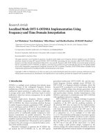
Figure 1: Face representation using space-localized basis images.
2. LOCAL FEATURE EXTRACTION TECHNIQUES
A number of recent algorithms aim at obtaining face rep-
resentations using (a linear combination of) space-localized
images roughly associated with the components of typical
faces such as eyes, nose, and mouth, as in Figure 1.
The individual images form a (possibly nonorthogonal)
basis, and the set of coefficients may be interpreted as the
face “signature” related to the specific basis. In the follow-
ing, we present the main characteristics of three distinct so-
lutions for obtaining such localized images. The general set-
ting is as follows: the available N training images are orga-
nized as a mat rix X, where a column consists of the raster-
scanned p pixel values of a face. We denote by B the set of m
basis vectors, and by H the matrix of projected coordinates
of data matrix X onto basis B. If the number of basis vectors
is smaller than the length of the image vectors forming X,we
get dimensionality reduction. On the contra ry, if the number
of basis images exceeds training data dimensionality, we ob-
tain overcomplete representations. As a consequence, we may
write
X
 BH,(1)
where X
∈ R
pxN
, B ∈ R
pxm

,andH ∈ R
mxN
.Different linear
techniques impose specific constraints on B and/or H,and
some yield spatial ly localized basis images.
2.1. Local nonnegative matrix factorization
Nonnegative matrix factorization (NMF) [15]hasbeenre-
cently introduced as a linear projection technique that im-
poses nonnegativity constraints on both B and H matrices
during learning. The method resembles matrix decomposi-
tions techniques such as positive matrix factorization [16],
and has found many practical applications including chemo-
metric or remote-sensing data analysis. The basic idea is that
only additive combinations of the basis vectors are allowed,
following the intuitive scheme of combining parts to form a
whole. Referring to (1), NMF imposes the following restric-
tions:
B,H
≥ 0. (2)
Unlike simulation results reported in [15], the images pro-
vided by NMF, when applied to human faces, still maintain
a holistic aspect, particularly in case of poorly aligned im-
ages, as was previously noted by several authors. In order
to improve localization, a local version of the algorithm has
been proposed in [12] that imposes the follow ing additional
constraints: (a) maximum sparsity of coefficients matrix H;
(b) maximum expressiveness of basis vectors B (keep only
those coefficients bearing the most important information);
(c) maximum orthogonality of B. The following equations
describe the updating procedure for B and H:

H
aj
←−




H
aj

i

B
T

ai
X
ij

BH

ij
,
B
ia
←− B
ia

j
X

ij
[BH]
ij

H
T

ja
,
B
ia
←−
B
ia

j
B
ja
.
(3)
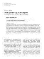
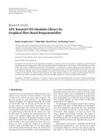
Examples of basis vectors obtained by performing LNMF on
AR database images are presented in Figure 2(a).
2.2. Independent components analysis
Natural images are highly redundant. A number of authors
argued that such redundancy provides knowledge [17], and
that the role of the sensory system is to develop factorial rep-
resentations in which the dependencies between pixels are
separated into statistically independent components. While
in PCA and LDA the basis vectors depend only on pairwise
relationships among pixels, it is argued that higher-order

statistics are necessary for face recognition, and ICA is an ex-
ample of a method sensible to such statistics. Basically, given
a set of linear mixtures of several statistically independent
components, ICA aims at estimating both the mixing ma-
trix and the source components based on the assumption of
statistical independence.
There are two distinct possibilities to apply ICA for face
recognition [13]. The one of interest from the perspective of
the present paper organizes the database into a large matrix,
whereas every image is a different column. In this case, images
are random variables and pixels are outcomes (independent
trials). We look for the independence of images or functions
of images. Two i and j images are independent if, when mov-
ing across pixels, it is not possible to predict the value taken
by a pixel on image i based on the value taken by the same
pixel on image j. The specific computational procedure in-
cludes two steps [13].
(a) Perform PCA to project original data into a lower-
dimensional subspace: this step both eliminates less
significant information and simplifies further process-
ing, since resulting data is decorrelated (and only
higher-order dependencies are to be separated by
ICA). Let V
PCA
∈ R
pxm
be the matrix whose columns
represent the first m eigenvectors of the set of N train-
ing images, and C
∈ R

mxN
the corresponding PCA co-
efficients matrix, we may write X
= V
PCA
∗ C.
(b) ICA is actually performed on matrix V
T
PCA
, a nd the in-
dependent basis images are computed as B
= W ∗
V
T
PCA
, where the separating matrix W is obtained with
the InfoMax method [18] (since directly maximizing
the independence condition is difficult, the general
I. B. Ciocoiu and H. N. Costin 3
(a) (b)
(c) (d)
Figure 2: Examples of basis vectors for AR image database: (a) LNMF; (b) ICA; (c) NMFsc; (d) LPP.
approach of most ICA methods aims at optimizing an
appropriate objective function whose extreme occurs
when the unmixed components are independent; sev-
eral distinct types of objective functions are commonly
used, e.g., InfoMax algorithm maximizes the entropy
of the components). The set of projected coordinates
on ICA subspace (the set of coefficients that linearly
combine the basis images in order to reconstruct the

original face images) is computed as H
T
= C ∗ W
−1
.
Due to somehow contradictory comparative results be-
tween ICA and PCA presented in the literature, a systematic
analysis has been reported in [19] in terms of algorithms and
architectures used to implement ICA, the number of sub-
space dimensions, distance metric, and recognition task (fa-
cial identity versus expression). Results indicate that specific
ICA design strategies are superior to standard PCA, although
the task to be performed remains the most important fac-
tor. Examples of basis images obtained by ICA-InfoMax ap-
proach are presented in Figure 2(b) (Matlab code is available
at />∼marni/code.html).
2.3. NMF with sparseness constraints
A r andom variable is called sparse if its probability density
is highly peaked at zero and has heavy tails. Within the gen-
eral setting expressed by (1), sparsity is an attribute of the
activation vectors grouped in the lines of coefficients ma-
trix H, the set of basis images arranged in the columns of
B, or both. While standard NMF does yield a sparse rep-
resentation of the data, there is no effective way to control
the degree of sparseness. Augmenting standard NMF with
the sparsity concept proved useful for dealing with overcom-
plete representations (i.e., cases where the dimensionality of
the space spanned by decomposition is larger than the effec-
tive dimensionality of the input space). While not present in
standard NMF definition, sparsity is taken into account in

LNMF and nonnegative sparse coding [14]. In fact, the lat-
ter enables the control over the (relative) sparsity level in B
and H by defining an objective function that combines the
goals of minimizing the reconstruction error and maximiz-
ing the sparseness level. Unfortunately, the optimal values of
the parameters describing the algorithm are set by extensive
4 EURASIP Journal on Image and Video Processing
trial-and-error experiments. This shortcoming is eliminated
in a more recent contribution of the same author, which
proposed a method termed NMF with sparseness constraints
(NMFsc) [14]. Sparseness of an n-dimensional vector x is de-
fined as follows:
sparseness (x)
=
√
n −




x
i






x
2

i
√
n − 1
. (4)
The algorithm proceeds by iteratively performing a gradient
descent step on the (Euclidean distance type) objective func-
tion, as in (5), followed by projecting the resulting vectors
onto the constraint space:
B
= B − μ
B
(WH − X)H
T
. (5)
The projection operator is the key element of the whole pro-
cessing procedure, which sets explicitly the L
1
and L
2
norms
of the basis components, and is fully described in [14]. Ex-
amples of basis images obtained after applying NMFsc on
AR face database images are presented in Figure 2(c) (Matlab
code is available at sinki.fi/patrik.hoyer/).
2.4. Locality-preserving projections
Linear subspace projection techniques such as PCA or LDA
are unable to approximate accurately data lying on nonlin-
ear submanifolds hidden in the face space. Although several
nonlinear solutions to unveil the structure of such manifolds
have been proposed (Isomap [20], LLE [21], Laplacian eigen-

maps [22]), these are defined only on the training set data
points, and the possibility of extending them to cover new
data remains largely unsolved (efforts towards tackling this
issue are reported in [23]). An alternative solution is to use
methods aiming at preserving the local structure of the man-
ifold after subspace projection, which should be preferred
when nearest neighbor classification is to be subsequently
performed. One such method is Locality-preserving projec-
tions (LPPs) [24]. LPP represents a linear approximation
of the nonlinear Laplacian eigenmaps introduced in [22].
It aims at preserving the intrinsic geometry of the data by
forcing neighboring points in the original data space to be
mapped into closely projected data. The algorithm starts by
defining a similarity matrix S,basedona(weighted)k near-
est neighbors graph, whose entry S
ij
represents the edge be-
tween training images (graph nodes) x
i
and x
j
. Gaussian-
type weights of the form S
ij
= e
−(x
i
−x
j


2
)/σ
have been pro-
posed in [24], although other choices (e.g., cosine type) are
also possible. Based on matrix S, a special objective function
is constructed, enforcing the locality of the projected data
points by p enalizing those points that are mapped far apart.
Basically, the approach reduces to finding a minimum eigen-
value solution to the following generalized eigenvalue prob-
lem:
XLX
T
b = λXDX
T
b,(6)
where D =

i
S
ij
and L = D − S (Laplacian matrix). The
components of the subspace projection matrix B are the
eigenvectors corresponding to the smallest eigenvalues of the
problem above.
Rigorous theoretical grounds are related tooptimal lin-
ear approximations to the eigenfunctions of the Laplace-
Bertrami operator on the manifold and are extensively pre-
sented in [24] (Matlab code is available at
.uchicago.edu/
∼xiaofei). When applied to face image analy-

sis, the method yields the so-called Laplacian faces, examples
of which are presented in Figure 2(d).
Remark 1. Another interesting manifold learning algorithm
calledOPRA(orthogonalprojectionreductionbyaffinity)
has been recently proposed [25], which also starts by con-
structing a weighted graph that models the data space topol-
ogy. This affinity graph is built in a manner similar to the
one used in local linear embedding (LLE) technique [21],
and expresses each data point as a linear combination of (a
limited number of) neighbors. The advantage of OPRA over
LLE is that the mapping between the original data and the
projected one is made explicit through a linear transforma-
tion, whereas in LLE this mapping is implicit, making it dif-
ficult to generalize to new test data. Compared to LPP, OPRA
preserves not only the locality but also the geometry of lo-
cal neighborhoods. Moreover, the basis vectors obtained by
performing OPRA are orthogonal, whereas projection direc-
tions obtained by LPP are not. When class labels are available,
as in our case, the algorithm is to be used in its supervised
version, namely an edge is present between two nodes in the
affinity graph only if the two corresponding data samples be-
long to the same class.
3. EXPERIMENTAL RESULTS
3.1. Image database preprocessing
AR database contains images of 116 individuals (63 males
and 53 females). Original images are 768
× 576 pixels in
size with 24-bit color resolution. The subjects were recorded
twice at a 2-week interval, and during each session, 13 con-
ditions with varying facial expressions, illumination, and oc-

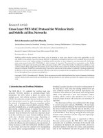
clusion were used. In Figure 3, we present examples from
this database. As in [26], we used as training images two
neutral poses of each person captured on different days (la-
beled AR01
1
and AR01
2
in Figure 3),while the testing set
consists of pairs of images for the remaining 12 condi-
tions, AR02, , AR13, respectively. More specifically, images
AR02, AR03, and AR04 are used for testing the performances
of the analyzed techniques to deal with expression variation
(smile, anger, and scream), images AR05, AR06, and AR07
are used for illumination variability, and the rest of the im-
ages are related to occlusion (eyeglasses and scarf), with vari-
able illumination conditions. The subset of the AR database
is the same as in [ 26], and was kindly provided by the au-
thor. First, pose normalization has been applied in order to
align all database faces, according to the (manually) local-
ized eye positions. Next, only part of a face inside an ellipti-
cal region was selected, in order to avoid the influence of the
background. The size of each reduced image is 40
×48 pixels,
and when considering the elliptical region only, each image
I. B. Ciocoiu and H. N. Costin 5
AR01
1
AR01
2
AR02 AR03 AR04 AR05

AR06 AR07 AR08 AR09
AR10 AR11 AR12 AR13
Figure 3: Example of one individual from the AR face database: (1) neutral, (2) smile, (3) anger, (4) scream, (5) left light on, (6) right light
on, (7) both lights on, (8) sunglasses, (9, 10) sunglasses left/right light, (11) scarf, (12, 13) scarf left/right light.
is represented using 1505 pixels. No illumination normaliza-
tion procedure has been applied, since we are directly inter-
ested in a comparative analysis of the algorithms per se deal-
ing with illumination variability (although preliminary tests
using histogram equalized images indicate that recognition
accuracy deteriorates in most cases).
Olivetti database comprises 10 distinct images of 40 per-
sons, represented by 112
× 92 pixels, with 256 gray levels. All
the images were taken against a dark homogeneous back-
ground with the subjects in an upright frontal position, w ith
tolerance for some tilting and rotation of up to about 20
degrees. In order to enable comparisons with previously re-
ported results, we randomly selected 5 images per person for
the training set, the remaining 5 images were included in the
test set, and average recognition rates over 20 distinct trials
were computed.
3.2. Comparative performance analysis
In this section, we present simulation results for the algo-
rithms described in Section 2. The performances are given in
terms of recognition accuracy and are compared to results
obtained by performing standard PCA. The design items
taken into account are (a) the distance metric used: Euclidean
(L2), Manhattan (L1), cos (cosine of the angle between the
compared vectors, cos(x, y)
= (x ·y)/(xy)); (b) projec-

tion subspace dimension: the dimension of the feature space,
equal to the number of basis vectors used, is set to 50, 100,
150, and 200 dimensions.
In order to make the evaluation, we conducted a rank-
based analysis as follows: for each image/dimension com-
bination, we ordered the performance rank of each algo-
rithm/distance measure combination (the highest recogni-
tion rate got rank 1, and so on) regardless of the subspace
dimension. This yielded a total of 11 rank numbers for each
case: expression variation, illumination variation, glasses,
and scarf. Then, we computed a sum of ranks for each of
the algorithms over all the cases, and ordered the results (the
lowest sum indicates the best overall performance).
3.2.1. Facial expression recognition
The capacity of the methods to deal with expression variabil-
ity was tested using images labeled AR02, AR03, and AR04,
and results are presented in Ta ble 1. Algorithm NMFsc using
L
1
distance deals best with smile expression, while LNMF +
L
1
and ICA + COS combinations give best results for smile
and anger expressions, respectively. Recognition accuracies
of up to 96% are obtained for AR02 and AR03 images, while
62.4% is reached for the most difficult task AR04. Rank anal-
ysis conducted on combined AR02, AR03, and AR04 im-
ages reveals that the LNMF + L
1
approach outperforms the

other competitors, followed by ICA + L
1
/L
2
algorithm, as
presented in Table 2. Generally, greater basis dimensionality
tends to be favored. L
1
norm yields the best results, followed
by L
2
and the cosine metric. While perfor ming second best
for smile expression, standard PCA occupies a middle posi-
tion on the combined expression rank analysis results.
3.2.2. Changing illumination conditions
Changing illumination conditions are reflected in images
AR05, AR06, and AR07, and recognition performances are
given in Ta ble 3. The ICA-InfoMax approach ranks best on
both individual tests and combined analysis, with accuracies
of up to 98%, 97%, and 89%, respectively. Laplacian faces
perform second best, followed by PCA. Greater basis dimen-
sionality yields better results, while no distance metric is f a-
vored. Standard PCA is placed again on a middle position,
better than LNMF and NMFsc algorithms. It is worth noting
6 EURASIP Journal on Image and Video Processing
Table 1: Recognition rates for AR database/expression variability.
Expression
AR02 AR03 AR04
m = 50 m = 100 m = 150 m = 200 m = 50 m = 100 m = 150 m = 200 m = 50 m = 100 m = 150 m = 200
L2 83.7 72.2 64.5 82.4 89.7 92.3 93.1 95.3 41.4 46.1 39.7 49.5

L1
92.7 92.3 86.3 95.7 93.1 94 94.8 96.5 53 56.8 54.7 61.5
LNMF + cos
76 64.1 59.4 73.9 84.6 90.6 92.7 93.6 34.2 38.9 33.3 41.8
L2 91 92.3 92.7 91.8 91.4 92.3 93.1 93.6 49.1 52.1 53 55.1
ICA + L1
91 92.7 91.8 91.4 93.1 93.6 93.6 94.4 51.7 55.1 55.5 57.2
cos
89.7 90.6 91.4 89.7 89.3 90.6 91 90.1 58.1 62.4 60.6 61.1
L2 79 91 92.7 93.1 67.9 85.9 89.7 88.4 29.5 38.9 38.9 44.4
NMFsc + L1
88.9 95.7 96.1 93.6 86.7 91.8 92.7 90.6 41.8 44 46.5 46.5
cos
73.5 88 91.8 91.8 65.8 85.4 91 89.3 26.9 37.1 38.9 45.7
Laplacian faces 73.9 87.2 89.7 89.7 83.7 91.4 91.8 91.4 17 30.8 29.5 30.8
PCA
91 94.4 95.3 95.7 88 89.7 89.7 90.6 47.4 52.5 52.5 52.5
Table 2: Rank-based analysis results.
Algorithm/distance Expression rank Illumination rank Glasses rank Scarf rank Sum of ranks
ICA-cos 14 6 3 6 29
ICA-L1
10 8 9 3 30
ICA-L2
12 7 6 9 34
Laplacian
27 9 23 15 74
LNMF-L1
539182486
NMFsc-L1
13 31 22 31 95

PCA
15 25 24 39 103
NMFsc-cos
20 26 28 31 105
NMFsc-L2
22 29 30 27 108
LNMF-L2
17 40 37 32 126
LNMF-cos
23 34 38 32 127
that recognition accuracies are significantly different for left
and right illumination directions, although the use of an ap-
propriate illumination normalization procedure could have
changed this conclusion.
3.2.3. Occlusion
Occlusion is one of the situations that hopefully should be
better tackled by local-based techniques compared to holis-
tic ones such as PCA. AR database provides two kinds of
partially occluded images, using sunglasses (images AR08)
and scarf (images AR11). Due to length constraints, we only
present in Table 4 results for eyeglasses occlusion, although
both cases show a sig nificant general decrease of the recog-
nition performances, especially when the illumination con-
ditions are changing. Recognition accuracies do not exceed
47%, while differences between left and right illumination
directions are maintained.
3.2.4. Pose variation
In Table 5 we give simulation results for the Olivetti database,
which present significant pose variation, while illumination
conditions are better controlled. LNMF + L

1
and OPRA faces
method yield the best results, followed by PCA and ICA +
COS, and all algorithms show rather limited dependence on
the subspace dimension. A key observation related to us-
ing OPRA in its supervised version must be made: since the
method relies on the assumption that each data point may
be approximated by a linear combination of its k nearest
neighbors belonging to the same class, we could not use this
method in case of AR database, where only 2 training sam-
ples per class are available.
4. CONCLUSIONS
We conducted an extensive set of experiments in order to
provide a comparative analysis of the recognition perfor-
mances of several modern subspace projection algorithms in
terms of distance metric used, number of selected features,
and sources of variability on AR and Olivetti face databases.
The study revealed that ICA implemented by the InfoMax
algorithm seems best suited for face oriented tasks, outper-
forming clearly all other solutions in case of AR database.
While explaining the exact reason for this remarkable per-
formance needs further study, we may note that searching
I. B. Ciocoiu and H. N. Costin 7
Table 3: Recognition rates for AR database/illumination variability.
Illumination
AR05 AR06 AR07
m = 50 m = 100 m = 150 m = 200 m = 50 m = 100 m = 150 m = 200 m = 50 m = 100 m = 150 m = 200
L2 17 29.5 36.3 25.6 11.9 13.6 11.9 8.9 2.1 6.4 3.4 1.7
L1
20 32.9 38.4 28.2 8.1 20 13.6 11.5 1.2 1.7 2.1 2.1

LNMF + cos
46.5 48.3 53.8 57.2 30.7 23 20.9 10.2 17 15.3 14.5 17
L2 95.3 97.4 97.4 98.3 89.3 92.7 93.6 93.1 73.9 79.5 80.3 79.9
ICA + L1
95.3 97 97.8 97.4 90.6 92.3 94.8 92.7 75.6 79 79.5 79
cos
95.7 97.4 97.4 97 94 97.4 97.8 97.4 88.4 89.3 89.3 88.9
L2 44 56 76 71.3 9.8 22.6 22.2 34.2 11.1 15.3 23.5 27.3
NMFsc + L1
43.1537376 9.4 26.5 17.9 32 5.1 10.6 19.6 20.9
cos
55.1 61.9 77.3 73.9 11.9 27.7 25.6 36.7 22.6 24.3 34.6 37.6
Laplacian faces 79.5 91.5 94.4 95.3 72.6 93.2 93.1 92.7 56.8 87.2 91.4 89.7
PCA
73.5 77.3 80.7 81.2 16.2 20.9 21.3 21.3 58.9 67 70 71.3
Table 4: Recognition rates for AR database/occlusion (sunglasses).
Occlusion sunglasses
AR08 AR09 AR10
m = 50 m = 100 m = 150 m = 200 m = 50 m = 100 m = 150 m = 200 m = 50 m = 100 m = 150 m = 200
L2 7.7 6.8 5.5 7.2 5.1 5.5 3.4 3.8 5.1 2.5 3.8 3.8
L1
22.2 20.5 17 28.6 10.6 14.1 12.8 14.1 9 6.4 5.1 7.7
LNMF + cos
8.1 6 2.5 6.8 4.2 4.7 3 3.8 4.7 2.1 2.1 3
L2 28.2 34.6 34.6 35.9 26 27.7 29 29.5 26 29 29.5 30.3
ICA + L1
26.9 29.5 30.7 32.9 27.3 25.2 26 28.6 26.5 25.6 27.3 27.3
cos
39.3 43.6 45.3 47.4 36.3 38.9 40.6 40.6 31.6 36.7 36.7 38
L2 10.2 9.8 11.5 17 5.5 8.1 7.7 11.5 6.4 6.8 8.1 8.5

NMFsc + L1
18.3 14.5 15.3 23.9 9.4 9.4 8.1 11.1 5.5 6.4 7.7 9.4
cos
9.8 9.4 9.8 18.3 4.2 7.2 7.2 11.1 5.1 6 6.4 7.7
Laplacian faces 8.9 15 17.9 18.3 4.7 6.8 11.5 12.4 4.7 8.9 8.9 9.4
PCA
8.5 8.5 10.2 11.1 11.5 12.4 13.2 13.2 8.9 9.8 9.4 9.8
Table 5: Recognition rates for Olivetti database.
m = 50 m = 100 m = 150 m = 200
L2 90.4 93.4 93.2 92.8
L1
92.3 95.1 94.4 94.3
LNMF + cos
89.1 92.9 91.7 91.1
L2 92 92.7 92.4 93
ICA + L1
92.3 93.3 92.8 93.7
cos
93.4 94.3 93.2 93.7
L2 89 91 89.9 90
NMFsc + L1
92 90.5 91.6 90.5
cos
91 92 90.8 92
Laplacian faces 91.1 90.7 89.9 90.7
OPRA faces
94.2 94.9 95 92.8
PCA
93.9 94.4 93.3 94.3
for most informative features (instead for most expressive

ones, as in PCA, or most discriminant, as in LDA) has been
previously proposed in the literature. Moreover, considering
recognition performances reported in an independent study
[26], we may conclude that ICA-InfoMax compares favor-
ably with two leading computer vision techniques, namely
Local Feature Analysis [27], and Bayesian PCA [28], where a
similar experimental setup based on AR database was used.
Based on overall results it is worth noting that, except for
expression recognition, manifold learning algorithms rank
amongst the top performers. Moreover, PCA also compares
favorably to most local representations (except for the occlu-
sion tasks), confirming the conclusions from [29].
Some other conclusions agree with previously reported
results, namely cosine and L
1
metrics are almost always supe-
rior to L
2
, and the dependence of the recognition rates on the
projection subspace dimension is not always clear (although
larger dimensions tend to be generally favored).
Some important aspects must be tackled if these ap-
proaches are to become important tools in face oriented ap-
plications. Reliable selection of significant basis vectors is
still an open problem, if the number of training images per
class is small. Basis vectors exhibiting invariance to common
transformations such as translations and in-plane rotations
8 EURASIP Journal on Image and Video Processing
are desirable. Finally, a key problem to be further addressed is
the identification of the conditions under which correct de-

compositions of faces into significant/generic parts emerge
[30].
REFERENCES
[1] S. G. Kong, J. Heo, B. R. Abidi, J. Paik, and M. A. Abidi, “Recent
advances in visual and infrared face recognition—a review,”
Computer Vision and Image Understanding,vol.97,no.1,pp.
103–135, 2005.
[2] W. Zhao, R. Chellappa, P. J. Phillips, and A. Rosenfeld, “Face
recognition: a literature survey,” ACM Computing Surveys,
vol. 35, no. 4, pp. 399–458, 2003.
[3] J. Lu, K. N. Plataniotis, and A. N. Venetsanopoulos, “Face
recognition using kernel direct discriminant analysis algo-
rithms,” IEEE Transactions on Neural Networks, vol. 14, no. 1,
pp. 117–126, 2003.
[4] M H. Yang, “Kernel eigenfaces vs. kernel fisherfaces: face
recognition using kernel methods,” in Proceedings of the 5th
IEEE International Conference on Automatic Face and Gesture
Recognition (FGR ’02), pp. 215–220, Washington, DC, USA,
May 2002.
[5] J. Yang, A. F. Frangi, J Y. Yang, D. Zhang, and Z. Jin, “KPCA
plus LDA: a complete kernel fisher discriminant framework
for feature extraction and recognition,” IEEE Transactions on
Pattern Analysis and Machine Intelligence, vol. 27, no. 2, pp.
230–244, 2005.
[6] J.Yang,X.Gao,D.Zhang,andJ Y.Yang,“KernelICA:anal-
ternative formulation and its application to face recognition,”
Pattern Recognition, vol. 38, no. 10, pp. 1784–1787, 2005.
[7] B. Heisele, P. Ho, J. Wu, and T. Poggio, “Face recognition:
component-based versus global approaches,” Computer Vision
and Image Understanding, vol. 91, no. 1-2, pp. 6–21, 2003.

[8] S. Lucey and T. Chen, “A GMM parts based face representation
for improved verification through relevance adaptation,” in
Proceedings of the IEEE Computer Society Conference on Com-
puter Vision and Pattern Recognition (CVPR ’04), vol. 2, pp.
855–861, Washington, DC, USA, June-July 2004.
[9] X. He, S. Yan, Y. Hu, P. Niyogi, and H J. Zhang, “Face recogni-
tion using Laplacianfaces,” IEEE Transactions on Pattern Anal-
ysis and Machine Intelligence, vol. 27, no. 3, pp. 328–340, 2005.
[10] J. Zhang, S. Z. Li, and J. Wang, “Manifold learning and ap-
plications in recognition,” in Intelligent Multimedia Processing
with Soft Computing, Springer, Heidelberg, Germany, 2004.
[11] FRVT 2002, 2004: Evaluation Report, .
[12] S. Z. Li, X. W. Hou, H. J. Zhang, and Q. S. Cheng, “Learning
spatially localized, parts-based representation,” in Proceedings
of IEEE Computer Society Conference on Computer Vision and
Pattern Recognition (CVPR ’01), vol. 1, pp. 207–212, Kauai,
Hawaii, USA, December 2001.
[13] M.S.Bartlett,J.R.Movellan,andT.J.Sejnowski,“Facerecog-
nition by independent component analysis,” IEEE Transactions
on Neural Networks, vol. 13, no. 6, pp. 1450–1464, 2002.
[14] P. O. Hoyer, “Non-negative matrix factorization with sparse-
ness constraints,” Journal of Machine Learning Research, vol. 5,
pp. 1457–1469, 2004.
[15] D. D. Lee and H. S. Seung, “Learning the parts of objects by
non-negative mat rix factorization,” Nature, vol. 401, no. 6755,
pp. 788–791, 1999.
[16] P. Paatero and U. Tapper, “Positive matrix factorization: a non-
negative factor model with optimal utilization of error esti-
mates of data values,” Environmetrics, vol. 5, no. 2, pp. 111–
126, 1994.

[17] H. B. Barlow, “Unsupervised learning,” Neural Computation,
vol. 1, no. 3, pp. 295–311, 1989.
[18] A. J. Bell and T. J. Sejnowski, “An information-maximization
approach to blind separation and blind deconvolution,” Neu-
ral Computation, vol. 7, no. 6, pp. 1129–1159, 1995.
[19] B. A. Drap er, K. Baek, M. S. Bartlett, and J. R. Beveridge, “Rec-
ognizing faces w ith PCA and ICA,” Computer Vision and Image
Understanding, vol. 91, no. 1-2, pp. 115–137, 2003.
[20] J. B. Tenenbaum, V. de Silva, and J. C. Langford, “A global ge-
ometric framework for nonlinear dimensionality reduction,”
Science, vol. 290, no. 5500, pp. 2319–2323, 2000.
[21] S. T. Roweis and L. K. Saul, “Nonlinear dimensionality reduc-
tion by locally linear embedding,” Science, vol. 290, no. 5500,
pp. 2323–2326, 2000.
[22] M. Belkin and P. Niyogi, “Laplacian eigenmaps for dimension-
ality reduction and data representation,” Neural Computation,
vol. 15, no. 6, pp. 1373–1396, 2003.
[23] Y. Beng io, J F. Paiement, P. Vincent, O. Delalleau, N. Le Roux,
and M. Ouimet, “Out-of-sample extensions for LLE, isomap,
MDS, eigenmaps, and spectral clustering,” in Proceedings of the
Annual Conference on Neural Information Processing Systems 16
(NIPS ’03), pp. 177–184, Vancouver, Canada, December 2003.
[24] X. He and P. Niyogi, “Locality preserving projections,” in Pro-
ceedings of the Annual Conference on Neural Information Pro-
cessing Systems 16 (NIPS ’03), Vancouver, Canada, December
2003.
[25] E. Kokiopoulou and Y. Saad, “Face recognition using OPRA
-faces,” in Proceedings of the 4th Internat ional Conference on
Machine Learning and Applications (ICMLA ’05), vol. 2005, pp.
69–74, Los Angeles, Calif, USA, December 2005.

[26] D. Guillamet and J. Vitri
`
a, “Classifying faces with non-
negative matrix factorization,” in Proceedings of the 5th Cata-
lan Conference on Artificial Intelligence (CCIA ’02), vol. 2504,
pp. 24–31, Castell
´
o de la Plana, Spain, 2002.
[27] P. S. Penev and J. J. Atick, “Local feature analysis: a general
statistical theory for object representation,” Network: Compu-
tation in Neural Systems, vol. 7, no. 3, pp. 477–500, 1996.
[28] B. Moghaddam and A. Pentland, “Probabilistic visual learning
for object representation,” IEEE Transactions on Pattern Anal-
ysis and Machine Intelligence, vol. 19, no. 7, pp. 696–710, 1997.
[29] K. W. Bowyer and P. J. Phillips, Empirical Evaluation Tech-
niques in Computer Vision, Wiley-IEEE Computer Society
Press, Hoboken, NJ, USA, 1998.
[30] D. Donoho and V. Stodden, “When does non-negative matrix
factorization give a correct decomposition into parts?” in Pro-
ceedings of the Annual Conference onNeural Information Pro-
cessing Systems 16 (NIPS ’03), Vancouver, Canada, December
2003.