Báo cáo hóa học: " Research Article Models for Gaze Tracking Systems Arantxa Villanueva and Rafael Cabeza" doc

Hindawi Publishing Corporation
EURASIP Journal on Image and Video Processing
Volume 2007, Article ID 23570, 16 pages
doi:10.1155/2007/23570
Research Article
Models for Gaze Tracking Systems
Arantxa Villanueva and Rafael Cabeza
Electronic and Electrical Engineering Department, Public University of Navarra, Arrosadia Campus, 31006 Pamplona, Spain
Received 2 January 2007; Revised 2 May 2007; Accepted 23 August 2007
Recommended by Dimitrios Tzovaras
One of the most confusing aspects that one meets when introducing oneself into gaze tracking technology is the wide variety, in
terms of hardware equipment, of available systems that provide solutions to the same matter, that is, determining the point the
subject is looking at. The calibration process permits generally adjusting nonintrusive trackers based on quite different hardware
and image features to the subject. The negative aspect of this simple procedure is that it permits the system to work properly but
at the expense of a lack of control over the intrinsic behavior of the tracker. The objective of the presented article is to overcome
this obstacle to explore more deeply the elements of a video-oculographic system, that is, eye, camera, lighting, and so for t h, from
a purely mathematical and geometrical point of view. The main contribution is to find out the minimum number of hardware
elements and image features that are needed to determine the point the subject is looking at. A model has been constructed based
on pupil contour and multiple lighting, and successfully tested with real subjects. On the other hand, theoretical aspects of video-
oculographic systems have been thoroughly reviewed in order to build a theoretical basis for further studies.
Copyright © 2007 A. Villanueva and R. Cabeza. This is an open access article distributed under the Creative Commons Attribution
License, which permits unrestricted use, distribution, and reproduction in any medium, provided the original work is properly
cited.
1. INTRODUCTION
The increasing capabilities of gaze tracking systems have
made the idea of controlling a computer by means of the eye
more and more realistic. Research in gaze tracking systems
development and applications has attracted much attention
lately. Recent advancements in gaze tracking technology and
the availability of more accurate gaze trackers have joined the
efforts of many researchers working in a broad spectrum of

disciplines.
The interactive nature of some gaze tracking applica-
tions offers, on the one hand, an alternative human com-
puter interaction technique for activities where hands can
barely be employed and, on the other, a solution for dis-
abled people who maintain eye movement control [1–3].
The most extreme case would be those people who can
only move the eyes—with their gaze being their only way
of communication—such as some subjects with amyotrophic
lateral sclerosis (ALS) or cerebral palsy (CP) among others.
Among the existing tracking technologies, the systems
incorporating video-oculography (VOG) use a camera or a
number of cameras and try to determine the movement of
the eye using the information obtained after studying the
images captured. Normally, they include infrared lighting to
produce specific effects in the obtained images. The nonin-
trusive nature of the trackers employing video-oculography
renders it as an attractive technique. Among the existing
video-oculographic gaze tracking techniques, we find sys-
tems that determine the eye movement inside its orbit and
systems that find out the gaze direction in 3D, that is, line
of sight (LoS). If the gazing area position is known, the ob-
served point can be deduced as the intersection between LoS
and the specific area, that is, point of regard (PoR). In the pa-
per, the term gaze is used for both PoR and LoS, since both
are the consequence of the eyeball 3D determination.
Focusing our attention on minimal invasion systems, we
find in the very beginning the work by Merchant et al. [4]
in 1974 employing a single camera, a collection of mirrors,
and a single illumination source to produce the desired ef-

fect. Several systems base their technology on one camera
and one infrared light such as the trackers from LC [5]or
ASL [6]. Some systems incorporate a second lighting, as the
one from Eyetech, [7] or more in order to create specific re-
flection patterns on the cornea as in the case of Tobii [8].
Tomon o e t a l. [9] used a system composed of three cameras
and two sources of differently polarized light. Yoo and Chung
[10] employ five infrared lights and two cameras. Shih and
Liu [11] use two cameras and three light sources to build
2 EURASIP Journal on Image and Video Processing
their system. The mathematical rigor of this work makes it
the one that most closely resembles the work dealt with in
this paper. Zhu and Ji [12] propose a two-camera-based sys-
tem and a dynamic model for head movement compensa-
tion. Beymer and Flickner [13]presentasystembasedon
four cameras and two lighting points to differentiate head
detection and gaze tracking. Later, and largely based on this
work, Brolly and Mulligan [14] reduce the system to three
cameras. A similar solution as the one by Be ymer et al. is
proposed by Ohno and Mukawa [15]. Some interesting at-
tempts have been carried out to reduce the system hardware
such as the one by Hansen and Pece [16] using just one cam-
era based on the iris detection or the work by Wang et al.
[17].
It is surprising to find the wide variety of gaze tracking
systems which are used with the same purpose, that is, to de-
tect the point the subject is looking at or gaze direction. How-
ever, their basis seems to be the same; the image of the eye
captured by the camera will change when the eye rotates or
translates in 3D space. The objective of any gaze estimation

system is clear; a system is desired that p ermits determining
thePoRfromcapturedimagesinfreeheadmovementsitua-
tion. Consequently, the question that arises is evident: “what
are the features of the image and the minimum hardware that
permit computing unequivocally the gazed point or g aze di-
rection?”
This study tries to analyze in depth the mathematical
connection between the image and the gaze. Analyzing this
connection leads to the establishment of a set of guidelines
and premises that constitute a theoretical basis from which
useful conclusions are extracted. The study carried out shows
that, assuming that the camera is calibrated and the position
of screen and lighting are known with respect to the camera,
two LEDs and a single camera are enough to estimate PoR.
On the other hand, the position of the glints in the image and
the pupil contour are the needed features to solve gaze posi-
tion. The paper tries to reduce some cumbersome mathemat-
ical details and focus the reader’s attention on the obtained
conclusions that are the main contribution of the work [18].
Several referenced works deal with geometrical theory of gaze
tracking systems. The works by Shih and Liu [11], Beymer
and Flickner [13], and Ohno and Mukawa [15] are the most
remarkable ones. Recently, new studies have been introduced
such as the one by Hennessey et al. [19]orGuestrinand
Eizenman [20]. These are based on a single camera and mul-
tiple glints. The calibration process proposed by Hennessey
et al. [19] is not based on any system geometry. The system
proposed by Guestrin and Eizenman [20] proposes a rough
approximation when dealing with refraction. Both use multi-
ple points calibration processes that compensate for the con-

sidered approximations.
An exhaustive study of a tracker requires an analysis of
the alternative elements involved in the equipment of which
the eyeball represents the most complex. A brief study of its
most relevant characteristics is proposed in Section 2. Subse-
quently, in Section 3, alternative solutions are proposed and
evaluated to deduce the most simple system. Section 4 tries
to validate the model experimentally and finally the conclu-
sions obtained are set out in Section 5.
Nasal side
Visual axis
β
Optical axis
Te mp or al s id e
Nodal points
NN

Pupil
Optical nerve
Fovea
Figure 1: Top view of the right eye.
2. THE EYEBALL
Building up a model relating the obtained image with gaze
direction requires a deeper study of the elements involved in
the system. The optical axis of the eye is normally considered
as the symmetry axis of the individual eye. Consequently, the
center of the pupil can be considered to be contained in the
optical axis of the eyeball. The visual axis of the eye is nor-
mally considered as an acceptable approximation of the LoS.
When looking at some point, the eye is oriented in such a way

that the observed object projects itself on the fovea, a small
area with a diameter of about 1.2
◦
in the retina with a high
density of cones that are responsible for high visual detail dis-
crimination (see Figure 1). The line joining the fovea to the
object we are looking at, crossing the nodal points (close to
the cornea), can be approximated as the visual axis of the eye.
This is considered to be the line going out from the fovea
through the corneal sphere center. The fovea is slightly dis-
placed from the eyeball back pole. Consequently, there is an
angle of 5
± 1
◦
between both axes, that is, optical and vi-
sual axes, horizontally in the nasal direction. A lower angle
2-3
◦
can be specified vertically too, although there is a con-
siderable personal variation [21]. In this first approach, the
horizontal offset is considered since it is widely accepted by
the eye tracking community. The vertical deviation is obvi-
ated since it is smaller and the most simplified version of the
eye is desired.
Normally, gaze estimation systems find out first the 3D
position of the optical line of the eye to deduce the visual
one. To this end, not only the angular offset between axes is
necessary, but also the direction in which this angle must be
applied. In other words, we know that optical and visual axes
present an angular offset in a certain plane, but the position

of this plane when the user looks at a specific point is needed.
In Figure 2, the optical axis is shown using a dotted line. The
solid lines around it present the same specific angular offset
with respect to the dotted line and a ll of them are possible
visual axes if no additional information is introduced.
To find out this plane, that is, eyeball 3D orientation,
some knowledge about eyeball kinematics is needed. The
arising difficulties lead to eyeball kinematics being frequently
avoided by many tracker designers. The position of the opti-
cal axis 3D l ine is normally modeled by means of consecutive
rotations about the world coordinate system, that is, vertical
A. Villanueva and R. Cabeza 3
Optical axis
Figure 2: The dotted line represents the optical axis of the eye. The
solid lines are 3D lines presenting the same angular offset with re-
spect to the optical line and consequently possible visual axis candi-
dates.
1
4
3
2
Figure 3:Thenaturalrotationoftheeyeballwouldbetomovefrom
1-2 in one step following the continuous line path. The same posi-
tion can be arrived by making successive rotations, that is, 1-4-2 or
1-3-2; however, the final orientations are different from the correct
ones (1-2).
and horizontal or horizontal and vertical. However, the eye
does not rotate from one point to the other by making con-
secutive rotations. The movement is achieved in just one step
as is summarized in Listing’s Law [ 21]. The alternative ways

to model optical axis movement can lead to inconsistencies
in the final eye orientation.
Let us analyze the next example sketched in Figure 3.Let
us consider the cross a s the orientation of the eye; that is, the
horizontal line of the cross would be contained in the opti-
cal and visual axes plane for position 1. The intrinsic nature
of the eyeball will accomplish the rotation from point 1 to
point 2 in just one movement following the path shown with
the solid line. The orientation of the cross achieved in this
manner does not agree with the ones obtained employing
the alternative ways 1-3-2, that is, horizontal rotation plus
vertical rotation, or 1-4-2, that is, vertical rotation plus hor-
izontal rotation. This situation disagrees with Donder’s law
which states that the orientation and the degree of torsion of
the eyeball only depend on the point the subject is looking
at and are independent of the route taken to reach it [21].
From the example, it is concluded that the visual axis posi-
tion would depend on the path selected since the plane in
which the angular offset should be applied is different for the
three cases.
Fry et al. [22] solve the disagreement introducing the
concept of false torsion in their eye kinematics theory which
states that if eye rotations are modeled by means of consec-
utive vertical and horizontal movements or vice versa, once
the vertical and horizontal rotations are accomplished an ad-
ditional torsion is required to locate the eyeball accordingly
with the orientation claimed by the Listing’s law. This supple-
mentary rotation depends on the previously rotated angles
and is called false torsion and it can b e approximated by
tan


α
2

=
tan

θ
2

tan

ϕ
2

,(1)
where θ, ϕ are the vertical and horizontal rotation angles per-
formed by the eye with respect to a known reference system
and α is the torsion angle around itself.
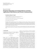
3. MODEL CONSTRUCTION
Gaze estimation process should establish a connection be-
tween the features provided by the technology, that is, image
analysis results, and gaze. The solution to this matter pre-
sented by most systems is to express this connection via gen-
eral purpose expressions such as linear or quadratic equa-
tions based on unknown coefficients [23], P
= Ω
T
F,where
P represents P oR, Ω is the unknown coefficients vector, and

F is the vector containing the image features and their pos-
sible combinations in linear, quadratic, or c ubic expressions.
The coefficients vector Ω is derived after the calibration of
the equipment that consists in asking the subject to look at
several known points on a screen, normally a grid of 3
× 3
or 4
× 4 marks uniformly distributed over the gazing area.
The calibration procedure permits systems with fully differ-
ent hardware and image features to work acceptably, but on
the other hand prevents researchers from determining the
minimal system requirements.
Our objective is to overcome this problem in order to
determine the minimum hardware and image features for a
gaze tracking system that permits an acceptable gaze estima-
tion by means of geometrical modeling. The initial system is
sketched in Figure 4. The optical axis of the eye contains three
principal points of the eyeball since it is approximated as its
symmetry axis, that is, A,eyeballcenter,C, corneal center,
and E, pupil center. The distance between pupil and corneal
centers is named as h andthecornealradiusasr
c
. In addition,
the angular offset between optical and visual axes is defined
as β. The pupil center and glint in the image are denoted as
p and g, respectively. All the features are referenced to the
camera projection center O.
We consider a model as a connection between the fixated
point or gaze direction, expressed as a function of subject
and hardware parameters describing the gaze tracking sys-

tem setup, and alternative features extracted from the image.
The study proposes alternative models based on known fea-
tures and on possible combinations and makes an evaluation
of its performance for a gaze tracking system. The evalua-
tion consists of a geometrical analysis in which mathematical
connection between the image features and 3D entities is an-
alyzed. From this point of view, the proposed model should
be able to determine the optical axis in order to estimate gaze
direction univocally and permit head free movement from
a purely geometrical point of view. Secondly, corneal refrac-
tion is considered, which is one of the most challenging as-
pects of the analysis to be introduced into the model. Lastly,
a further step is accomplished by analyzing the sensitivity of
4 EURASIP Journal on Image and Video Processing
LED
Camera
O
Eyeball
A
C
h
E
r
c
Cornea
Optical axis
β
Visual axis
Screen
p

g
Figure 4: The gaze tracking system.
the constructed model with respect to possible system inde-
termination such as noise.
The procedure selected to accomplish the work in the
simplest manner is to analyze separately the alternative fea-
tures that can be extracted from the image. In this manner, a
review of the most commonly used features employed by al-
ternative gaze tracking systems is carried out. The models so
constructed are categorized in three groups: models based on
points, models based on shapes,andhybrid models combining
points and shapes. The systems of the first group are based
on extracting features of the image which consist of single
points of the image and combine them in different ways. We
consider a point as a specific pixel described by its row and
column in the image. In this manner, we find in this group
the following models: the model based on the center of the
pupil, the model based on the glint, the model based on mul-
tiple glints, the model based on the center of the pupil and
the glint, and the model based on the center of the pupil
and multiple glints. On the other hand, the models based
on shapes involve more image information; basically these
types of systems take into account the geometrical form of
the shape of the pupil in the image. One model is defined in
this group, that is, the model based on the pupil ellipse. It is
straightforward to deduce that the models of the third group
combine both, that is, points and shapes, to sketch the sys-
tem. In this manner, we have the model based on the pupil
ellipse and the glint and the model based on the pupil ellipse
and multiple glints. Figure 5 shows a classification of the con-

structed models.
3.1. Geometrical analysis
The geometrical analysis evaluates the ability of the model to
compute the 3D position of the optical axis of the eye with
respect to the camera
1
in a free head movement scenario. Re-
1
If the gazwd point exact location is desired in screen coordinates, the
screen position with respect to the camera is supposed to be detrmined.
ferring to the optical axis, if two points among the three, that
is, A, C,andE, are determined with respect to the camera,
the optical axis is calculated as the line joining both points.
3.1.1. Models based on points
The center of the pupil in the image is a consequence of the
pupil 3D position. If affine projection is not assumed, the
center of the pupil in the image is not the projection of E
due to perspective distortion, but it is evident that it is ge-
ometrically connected to it. On the other hand, the g lint is
the consequence of the reflection of the lighting source on
the corneal surface. Consequently, the position of the glint or
glints in the image depends on the corneal sphere position,
that is, C. The models based on these features separately, that
is, p and g, are related to single points of the optical axis and,
consequently, cannot allow for optical axis estimation in a
free head movement scenario. Consequently, just the possi-
ble combinations of points will be studied.
(a) Pupil center and glint
Usually it is accepted that the pupil center corneal reflection
(PCCR) vector sensitivity with respect to the head position

is reduced. From the geometrical point of view of this work,
this approximation is not valid and creates a dependence be-
tween this vector value and the head position. Alternative ap-
proaches have been proposed based on these image features
using general purpose expressions; a thorough review of this
technique can be found in Morimoto and Mimica [24]. On
the other hand, an analytical head movement compensation
method based on the PCCR technique is suggested by Zhu
and Ji [12] in their gaze estimation model.
Our topic of discussion is to check if this two-feature
combination, not necessarily as a difference vector, can solve
the head constraint. So far, we know that the glint in the im-
age is directly related to corneal center C in the image plane.
On the other hand, the 3D position of the center of the pupil
is related to the location of the center of the pupil image. In
order to simplify the analysis, let us propose a rough approx-
imation of both features. If affine projection is assumed, the
center of the pupil in the image can be considered as the pro-
jection of E. In addition, if a coaxial location of the LED with
respect to the camera is given, the glint position can be ap-
proximated by the projection of C.Onecouldbackproject
the center of the pupil and the glint from the image plane
into 3D space, generating two lines and assuring that close
approximations of points E and C are contained within the
lines. One of them joins the center of the pupil p and the pro-
jection center of the camera, that is, r
m
,andr
r
connects the

glint g and the projection center of the camera (see Figure 6).
This hypothesis facilitates considerably the analysis and the
obtained conclusions are preserved for the real features.
As shown in the figure, knowing the distance between
C and E points, that is, h, does not solve the indetermina-
tion, since more than one combination of points in r
m
and
r
r
can be found having the same distance. Therefore, there
is no unique solution and we have an indetermination (see
A. Villanueva and R. Cabeza 5
Image features
Pupil center
Glint or multiple glints
Pupil elipse
Models
Models based on
points
Models based on
shapes
Hybrid models
Center of the pupil
Glint
Multiple glints
Center pupil+glint
Center pupil+mult. glints
Pupil elipse
Pupil elipse+glint

Pupil elipse+mult. glints
Figure 5: Models classification according to image features.
d(C, E)
Eyeball
A
C
E
Cornea
Optical axis
Lighting
r
r
r
m
Camera
Multiple
solutions
Image
Figure 6: Back-projected lines.
Figure 6). Therefore, once again the 3D optical position is
not determined.
(b) Pupil center and multiple glints
Following the law of reflection, it can be stated that, given an
illumination source L
1
, the incident and reflected rays and
the normal vector on the surface of reflection at the point of
incidence are coplanar in a plane denoted as Π
1
.Itisstraight-

forward to deduce that the center of the cornea C is contained
in the same plane since the normal line contained by the
plane crosses it. In addition, following the same reasoning,
the camera projection center O and the glint g will be also
contained in the same plane. If another lighting source L
2
is
introduced, a second plane Π
2
can be calculated containing
C.
If C is contained in the planes Π
1
and Π
2
, for the case
under study for which O
= (0,0,0),wehave
C
·

L
1
× g
1

= C·

L
2

× g
2

= 0. (2)
Considering the cornea as a specular surface and the reflec-
tion points on the cornea as C
i
for each L
i
(i = 1,2), the fol-
lowing vector equations can be stated from the law of reflec-
tion:
r
i
= 2

n
i
·l
i

n
i
− l
i
,
(3)
where r
i
is the unit vector in g

i
direction, l
i
is the unit vector
in (L
i
−C
i
) direction, and n
i
is the normal vector at the point
of incidence in (C
i
− C) direction.
Assuming that the corneal radius r
c
is known or can be
calibrated as will be shown later, C
i
can be expressed as a
function of C since the distance between them is known:
d

C
i
, C

=
r
c

. (4)
The solution for these equations (2)–(4) will be the corneal
center C as described in the works by Shih and Liu [11]and
Guestrin and Eizenman [20]. Consequently, using two glints
breaks the indetermination arising from the preceding model
based on the center of the pupil and one glint. In other words,
once C is found, the center of the pupil can be easily found
knowing r
m
and if the distance between pupil and corneal
centers, that is, h,isknownorcalibrated.Affine projection is
assumed for E; therefore, an error must be considered for the
pupil center since E is not exactly contained in r
m
.However,
no approximations have been considered for the glints and C
estimation.
3.1.2. Models based on shapes
It is already known that the projection of the pupil results
in a shape that can be approximated to an ellipse. Since in
this stage refraction is omitted, the pupil is considered to be
a circle and its projection is considered as an ellipse. The size,
position, orientation, and eccentricity of the obtained ellip-
tical shape are related to the position, size, and or ientation of
the pupil in 3D space. The projected pupil ellipse is geomet-
rically connected to the pupil 3D position and consequently
provides information about E position but not for C. There-
fore, the model based on the pupil ellipse does not allow for
the estimation of the optical axis of the eye.
3.1.3. Hybrid models

The last task to accomplish in the geometrical analysis of the
gaze tracking system would be to evaluate the performance
6 EURASIP Journal on Image and Video Processing
Pupil ellipse
Solution 2
Solution 1
Pupil back projection cone
(a)
Camera
Pupil back
projection cone
Potential
optical axes
Circular parallel s ections
E
E
E
r
r
(b)
Figure 7: (a) Multiple solutions collected in two possible orientations; (b) each plane intersects the cone in a circle resulting in an optical
axis crossing its center E.
of the models based on collections of features consisting of
points and shapes. Among the features consisting of a point,
it is of no great interest to select the center of the pupil since
considering the pupil ellipse as a working feature already in-
troduces this feature in the model.
(a) The pupil ellipse and glint
Once again and in order to simplify the analysis, we can de-
duce a 3D line, that is, r

r
, by means of the back projection of
the glint in the image, that is, g, which is supposed to con-
tain an approximation of C. The back projection of the pupil
ellipse would be a cone, that is, back projection cone, and
it could be assured that there is at least one plane that in-
tersects the cone in a circular section containing the pupil.
The matter to answer is actually the number of possible cir-
cular section planes and consequently the number of possi-
ble solutions that can be obtained from a single ellipse in the
image. The theory about conics claims that parallel intersec-
tions of a quadric result in equivalent conic sections. In the
case under study, considering the back projection cone as a
quadric, it is clear that if we find a plane with a circular sec-
tion for the specific quadric, that is, back projection cone, an
infinite number of pupils of different sizes could be defined
employing intersecting parallel planes. Moreover for the case
under analysis, that is, back projection cone of the pupil,
the analysis carried out provides two possible solutions, or
more specifically two possible orientations for planes result-
ing in circular sections of the cone. In summary, two groups
of an infinite number of planes can be calculated, each of
them intersecting the back projection cone in a circular shape
and containing a suitable solution for the gaze estimation
problem (see Figure 7(a)). The theory used to arrive at the
conclusion can be found in the work by Har tley and Zis-
serman [25] and more specifically in the book by Montes-
deoca [26] and is summarized in the appendix. Each possi-
ble intersection plane of the cone determines a pupil center
E and an optical axis that is calculated as the 3D line per-

pendicular to the pupil plane that crosses its center E (see
Figure 7(b)). It can be verified that the resulting pupil cen-
ters for alternative parallel planes belong to the same 3D line
[26].
Given r
r
, the solution is deduced if the distance between
the center of the pupil E and the corneal center C is known
or calibrated as will be explained later. The pupil plane for
which the optical axis meets the r
r
line at the known distance
from E will be selected as a solution. In addition, the inter-
section between the optical axis and the r
r
line will be the
corneal center C.
The preceding reasoning solves the selection of a certain
plane from a collection of parallel planes, but as already men-
tioned, two possible orientations of planes were found as
possible solutions. Therefore, the introduction of the glint
permits the selection of one of the planes for each one of the
two possible orientations. However, a more careful analysis
of the geometry of the planes leads one to conclude that just
one solution is possible and consequently represents a valid
model, as the second one requires the assumption that the
center of the cornea, C, remains closer to the camera than
the center of the pupil E, and it is assumed that the subject is
A. Villanueva and R. Cabeza 7
Camera

Optical axis 1
Solution 1
E
1
C
1
Solution 2
E
2
C
2
Choice at correct
distance
Optical axis 2
r
r
Cone
Figure 8: One of the solutions assumes that the cornea is closer
to the camera than the pupil center, which represents a nonvalid
solution.
looking at the screen [18]. Figure 8 shows the inconsistency
of the second solution (C
2
− E
2
) in its planar version.
(b) The pupil ellipse and multiple glints
It is already known that the combination of two glints and the
center of the pupil provides a solution to the tracking prob-
lem (see Section 3.1.1(b)). Therefore, at least the same result

is expected if the pupil ellipse is considered since it contains
the value of the center. In addition, the preceding section
showed that the ellipse and one glint were enough to sketch
the gaze, s o only a system performance improvement can be
expected if more glints are employed. The most outstanding
difference amongst models with one or multiple glints is the
fact that employing the infor mation provided exclusively by
the glints, the corneal center can be accurately determined.
The known point C must be located in one of the optical
axes calculated from the circular sections and crossing the
corresponding center E, and consequently the data about the
distance between C and E, that is, h, can be ignored.
3.2. Refraction analysis
The models selected in Section 3.1 are the model based on
the pupil center and two glints, the model based on the pupil
shape and one glint, and the model based on the pupil shape
and two glints. The refraction is going to modify the ob-
tained results and add new limitations to the model. For a
practical setup, a subject located at 500 mm from the camera
with standard eyeball dimensions, looking at the origin of
the screen (17

), that is, (0,0) point, the difference in screen
Pupil image
O
Virtual pupils
Projection cone
E
C
Refracted rays

Real pupil
Cornea
Figure 9: The cornea produces a deviation in the direction of the
light reflected back in the retina due to refraction. The consequence
is that the obtained image is not the simple projection of the real
pupil but the projection of a virtual shape. Each dotted shape in the
projection cone produces the same pupil image and can be consid-
ered as a virtual pupil.
coordinates whether considering refraction or not, that is,
thinking of the image as a plain projection of the pupil in the
image plane, is
∼26.52 mm, which represents a considerable
error (>1
◦
). Obviating refraction can result in non acceptable
errors for a gaze tracking system and consequently its effects
must be introduced in the model.
It must be assumed that a ray of light coming from the
back part of the eye suffers a refraction and consequently a
deviation in its direction when it crosses the corneal surface
due to the fact that the refraction indices inside the cornea
and the air are different. The obtained pupil image can be
considered as the projection of a virtual pupil and any par-
allel shape in the projection can be considered as a possible
virtual pupil as it is not physically located in 3D space. In
fact, there is an infinite number of virtual pupils. Figure 9 il-
lustrates the deviation of the rays coming from the back part
of the eye and the so-called virtual pupil.
The opposite path could be studied; a point belong ing to
the pupil contour in the image could be back projected by

means of the projection center of the camera. It is assumed
that the back-projection ray will intersect the cornea at a cer-
tain point and employing the refraction law, the path of the
ray coming into the cornea could be deduced. That should
intersect a point of the real pupil contour. The refraction af-
fects each ray differently. After refraction, the collection of
lines does not have a common intersection point or vertex
and the cone loses its reason to exist when refraction is con-
sidered.
Before any other consideration, the first conclusion de-
rived up to now is that the center of the cornea needs to
be known to apply refraction. Otherwise, the analysis from
8 EURASIP Journal on Image and Video Processing
the preceding paragraph could be applied at a ny point of r
r
.
Consequently, the model based on the pupil shape and the
glint fails this analysis since it does not accomplish a pre-
vious determination of the corneal center. Contrary to this
model, the one based on the pupil center and two glints makes
a prior computation of the corneal center; however, it can
no longer be assumed that the center of the real pupil is the
one contained in r
m
, but it is the center of the virtual pupil.
One could expect that E will be contained in a 3D line ob-
tained as a consequence of the refraction of r
m
when crossing
the cornea. This statement is unfortunately not true, since re-

fraction through a spherical surface is not a linear transfor-
mation. The pap er by Guestrin and Eizenman [20] implicitly
assumes this approximation as correct; that is, it assumes that
the image of the point E is the center of the pupil image. This
is strictly not correct since the distances between points be-
fore and after refraction through a spherical surface are not
proportional. Moreover, if this approximation is considered,
that is, the image of the center is the center of the image, the
errors for the tracking system are >1
◦
at some points. This
error, as expected, depends strongly on the setup values of
the gaze tracking session and can be compensated by means
of calibration, but considering our objective of a geometrical
description of the gaze estimation problem, this error is not
acceptable in a theoretical stage for our model requirements.
The model based on two glints and the shape of the pupil
provides the most accurate solution to the matter. The model
deduces the value of C employing exclusively the two glints
of the image. Considering refraction, it is already known that
the back-projected shape suffers a deformation at the corneal
surface. The center of the pupil should be a point at a known
distance d(C, E)
= h from C that represents the center of a
circle whose perimeter is ful ly contained in the refracted lines
of the pupil, and perpendicular to the line connecting pupil
and corneal centers. Mathematically, this can be described as
follows. First, the corneal center C is estimated assuming that
r
c

is known (see Section 3.1.1(b)).
(i) The pupil contour in the image is sampled to obtain
the set of points p
k
k = 0, , N. Each point can be
back projected through the camera projection center
O and the intersection with the corneal sphere cal-
culated as I(p
k
). From Snell’s Law, it is known that
na sin δ
i
= nb sin δ
f
,wherena and nb are the refrac-
tive indices of air and the aqueous humour in contact
with the back surface of the cornea (1.34), meanwhile
δ
i
and δ
f
are the angles of the incident a nd the re-
fracted rays, respectively, with respect to the normal
vector of the surface. Considering this equation for a
point of incidence in the corneal surface, the refraction
can be calculated as (see [27])
f
p
k
=

na
nb

i
p
k
−


i
p
k
·n
p
k

+




na
nb

2
− 1+

i
p
k

·n
p
k

2

n
p
k

,
(5)
where f
p
k
is the unit vector of the refracted ray at the
point of incidence I(p
k
), i
p
k
represents the unit vec-
tor of the incident ray from the camera pointing to
Pupil
C h
P
k
E
P
2

P
1
Π
Refracted rays
Cornea
−→
f
−→
i
−→
n
Back projected
pupil lines
Figure 10: Cornea and pupil after refraction. E is the center of a
circumference formed by the intersections of the plane Π with the
refracted ra ys. The plane Π is perpendicular to (C
− E) and the dis-
tance between pupil and corneal centers is h.
I(p
k
), and n
p
k
is the normal vector at that certain point
on the cornea. In this manner, for each point p
k
of
the image, the corresponding refracted line with di-
rection f
p

k
containing point I(p
k
) is calculated, where
k
= 0, , N.
(ii) The pupil will be contained in a planethat has (C
−
E) as nor mal vector having a distance of d(C, E) = h
with respect to C. Given a 3D point x
= (x, y, z)with
respect to the camera, the plane Π can be defined as
(C
− E)
h
.(x
− C)+h = 0. (6)
(iii) Once is defined, the intersection of the refracted lines
f
p
k
can be calculated, using (5)and(6), and a set of
points can be determined as P
k
, k = 0, , N. The ob-
tained shape fitted to the points must be a circumfer-
ence with its center in E:
d

P

1
, E

= d

P
2
, E

=··· =d

P
k
, E

. (7)
The pupil center E is solved numerically using equa-
tions like (7) to find out the constrained global optima (see
Figure 10). The nonlinear equations are given as constraints
of a minimization algorithm employing the iterative Nelder-
Mead (simplex) method. The objective function is the dis-
tance of the P
k
points to the best fitted circumference. The
initial value for the point E is the corneal center C.Theo-
retically, three lines are enough in order to solve the prob-
lem since three points are enough to determine a circle. But
in practice, more lines (about 20) are considered in order to
make the process more robust.
Once C and E are deduced, the optical axis estimation

is straightforward. Optical axis estimation permits us to cal-
culate the Euclidean transformation, that is, translation (C)
and rotation (θ and ϕ), performed by the eye from its pri-
mary position to the new position with respect to the camera.
Knowing the rotation angles, the additional torsion α is cal-
culated by means of1. Defining visual axis direction (for the
left eye) with respect to C as v
= (−sin β,0,cosβ)permits
A. Villanueva and R. Cabeza 9
us to calculate LoS direction with respect to the camera by
means of the Euclidean coordinate transformation:
C+R
α
R
θϕ
∗v
T
,(8)
where R
θϕ
is the rotation matrix calculated as a function of
the vertical and horizontal rotations of vector (C
− E)with
respect to the camera coordinate system and R
α
represents
the rotation matrix of the needed torsion around the optical
axis to deduce final eye orientation. The computation of the
PoR as the intersection of the gaze line with the screen plane
is straightforward.

3.3. Sensitivity analysis
From the prior analysis, the model based on two glints and
the shape of the pupil appears as the only potential model
for the gaze tracking system. In order to evaluate it exper-
imentally, the influence of some effects that appear when a
real gaze tracking system is considered such as certain intrin-
sic tolerances and noise of the elements composing the eye
tracker needs to be introduced.
Firstly, effects influencing the shape of the pupil such as
noise and pixelization have been studied. The pixelization ef-
fect has been measured using synthetic images. Starting from
elliptical shapes, images of size 200
× 200 have been assumed.
A pixel size of 13
× 13 μm is selected to discretize the el-
lipse according to the image acquisition device to be used
in the experimental test (Hamamatsu C5999). The noise has
been estimated as Gaussian from alternative images captured
by the camera employing well-known noise estimation tech-
niques [28]. This noise has been introduced in previously
discretized images. The obtained PoR is compared before and
after pixelization and before and after noise introduction.
The conclusion shows that a deviation in the PoR appears,
but the system can easily assume it since in the worst case
and taking into account both contributions, it remains un-
der acceptable limits for gaze estimation (
≤0.05
◦
).
The reduced size of the glint in the image introduces cer-

tain indetermination in the position of the corneal reflection
and consequently in the corneal center computation. The
glint can be found with alternative shapes in the captured
images. The way to proceed is to select a collection of real
glints, extracted from real images acquired with the already
known camera. The position of the glint center is calculated
employing two completely different analysis methods. The
first method extracts a thresholded contour of the glint and
estimates its center as the center obtained after fitting such a
border to an ellipse [13]. The second method binarizes the
image with a proper threshold and calculates the gravity cen-
ter of the obtained area. Images from different users and ses-
sions have been considered for the analysis and the differ-
ences between the glint values employing the two alternative
methods have been computed to extract consistent results
about the indetermination of the glint. The obtained results
show that, on average, an indetermination of
∼0.1 pixel can
be expected for the center of the glint in eye images for dis-
tances below 400 mm from the user to the camera, but it rises
to
∼0.2 pixel when the distance increases, leading the model
to nonacceptable errors (>1
◦
).
7
(0, 355)
6
(177.5, 355)
5

(355, 355)
17
(27, 277)
13
(100, 255)
12
(255, 255)
16
(328, 277)
8
(0, 177.5)
9
(177.5, 177.5)
4
(355, 177.5)
14
(27, 78)
10
(100, 100)
11
(255, 100)
15
(328, 78)
1
(0, 0)
2
(177.5, 0)
3
(355, 0)
Figure 11: Test sheet.

To reduce the sensitivity to glint indetermination, larger
illumination sources can be employed, by means of arrays of
illuminators. One interesting solution to explore, which has
been adopted by this study, is to increase the number of illu-
mination sources to obtain an average value for the point C.
It is already known that two glints can determine the center
of the cornea, when the locations of the illumination sources
are known. In this manner, if more than two illuminators
are employed, alternative pairs can be used to estimate the
pursued point and the calculated average. An increase in the
number of LEDs is supposed to reduce the sensitivity of the
model.
4. EXPERIMENTAL RESULTS
Ten users were selected for the test. The working distance
was selected in the range of 400–500 mm from the cam-
era. They had little or no experience with the system. They
were asked to fixate each test point for a time. Figure 11
shows the selected fixation marks uniformly distributed in
the gazing area w hose position is known (in mm) with re-
spect to the camera. The position in mm for each point is
shown. The obtained errors will be compared to the com-
mon value of 1
◦
of visual angle as system performance indi-
cator (a fixation is normally considered as a quasistable posi-
tion of gaze in 1
◦
area). During this time, ten consecutive im-
ages were acquired and grabbed for each fixation. The users
selected the eye they felt more comfortable with. They were

allowed to move the head between fixation points and they
could take breaks during the experiment. However, they were
asked to maintain their head fixed during each test point (ten
images).
10 EURASIP Journal on Image and Video Processing
Figure 12: The LEDs are attached to the inferior and lateral borders
of the test area.
Glint
extraction
Captured image
Pupil border
extraction
1
43
2
Figure 13: Analysis carried out.
The constructed model presents the following require-
ments.
(i) The camera must be calibrated [29].
(ii) Light source and screen positions must be known with
respect to the camera [18].
(iii) The subject eyeball parameters r
c
, β,andh must be
known or calibrated.
TheimageshavebeencapturedwithacalibratedHama-
matsu C5999 camera and digitalized by a Matrox Meteor
card with a resolution of 640
× 480 (RS-170). The LEDs
used for lighting have a spectrum centered at 850 nm. The

whole system is controlled by a dual processor Pentium at
1.7 GHz with 256 MB of RAM. Four LEDs were selected to
produce the needed multiple glints. They were located in
the lower part and its positions w ith respect to the camera
calculated ((
−189.07, −165.5) mm, (−77.91, −187.67) mm,
(98.59,
−191.33) mm, and (202.48, −152.78) mm), which re-
duces considerably the misleading possibility of partial oc-
clusions of the glints by eyelids when looking at differ ent
points of the screen because in this way the glints in the im-
age appear in the lower pupil half. Figure 12 shows a frontal
view of the LEDs area.
The images present a dark pupil and four bright glints as
shown in Figure 13. The next step was to process each im-
age separately to extract the glints coordinates [30] and the
contour of the pupil. It is not the aim of this paper to dis-
cuss the image processing algorithms used, distracting the
reader from the main contribution of the work, that is, the
mathematical model. The objective of the experimental tests
was to confirm the validit y of the constructed model. To this
end, the analysis of the images was supervised to minimize
the influence of the results of possible errors due to the im-
age processing algorithms used. The glints were supervised
by checking the standard deviation of each glint center po-
sition among the ten images for each subject’s fixation, and
exploring more carefully those cases for which the deviation
exceeded a certain threshold. For the pupil, deviations on the
ellipse parameters were checked in order to find inconsisten-
cies among the images. The errors were due to badly focused

images, subject’s large movement, or partially occluded eyes.
These images were eliminated from the analysis to obtain re-
liable conclusions.
Once the hardware was defined and in order to apply
the constructed model based on the shape of the pupil and
glints positions, some individual subject eyeball characteris-
tics need to be calculated, that is, r
c
, β,andh. To this end, a
calibration was performed. The constructed model based on
multiple glints and pupil shape permits, theoretically, deter-
mining this data by means of a single calibration mark and
applying the model already described in Section 3. Giving the
PoR as the intersection of the screen and LoS, model equa-
tions, that is, (2)–(4)and(6)–(8), can be applied to find the
global optima for the parameters that minimize the differ -
ence between model output and real mark position. Together
with the parameter values, the positions of C and E will be es-
timated for the calibration point. In Figure 14, the steps for
the subject calibration are shown.
In practice and to increase confidence in the obtained
values, three fixations were selected for each subject to es-
timate a mean value for eye parameters. For each subject, the
three points with lower variances in the extracted glint po-
sitions were selected for calibration. Each point among the
three permits estimating values for h, β,andr
c
.Thepersonal
eyeball parameters for each subject are given as the average
of the values obtained for the selected three points. The per-

sonal values obtained for the ten users are shown in Tables
1 and 2. It is evident that the sign of the angular offset was
directly related to the eye used for the test. Since the model
was constructed for the left eye, it is clear that a negative sign
indicates that the subject used the right eye to conduct the
experiment.
Once the system and the subject were calibrated, the per-
formance of the model was tested for two, three, and four
LEDs. Figure 15 shows the results obtained for users 1–5. For
each subject, black dots represent the real values for the fix-
ations. The darkest points show results obtained with four
LEDs. The lightest ones are the estimations by means of three
LEDs. The rest show the estimations of the model using two
LEDs. Figure 16 exhibits the same results for users 6–10.
Corneal refraction effects are more important as eye ro-
tation increases. The spherical corneal model presents prob-
lems in the limit between the cornea and the eyeball. The dis-
tribution of the used test points forces lower eye rotations
compared to other settings in which the camera is located
A. Villanueva and R. Cabeza 11
1 calibration point
Image features:
- Glints positions
- Pupil elipse
Calibration
Subject parameters
r
c
, β, h
Model defined for

the subject
Gaze estimation
Model HW calibrated
Figure 14: The personal calibration permits us to extract the physical parameters of the subject’s eyeball using one calibration point, the
captured image, and g aze estimation model information.
Table 1: Values for eyeball parameters obtained for subjects 1–5 by means of calibration, using three calibration points.
Subject12345
r
c
9.334 ± 0.83 9.103 ± 0.97 9.544 ± 0.88 9.875 ± 0.79 9.673 ± 1.03
h 5.034
± 0.83 4.730 ± 0.68 5.270 ± 0.41 5.565 ± 0.20 4.581 ± 0.97
β 6.25
± 0.76 4.15 ± 0.65 −4.49 ± 0.54 −3.36 ± 0.31 −5.16 ± 0.92
under the monitor. When the camera is located under the
monitor, the eye rotation increases and the refraction points
move toward the peripheral area of the cornea. In these cases,
system accuracy may decrease. A simulation is made with a
standard eyeball to evaluate the influence of refraction for
the points selected by using the model without refraction.
The average error for the points selected is
∼3
◦
, which ex-
ceeds the limit of 1
◦
, and the hig hest error ∼5
◦
appears for
the most extreme points in the corners for which the refrac-

tion effects increase. Consequently, it is necessary to consider
refraction for the selected distribution of p oints in the model.
It is clear that the errors due to refraction would increase for
cases in which larger eye rotations were accomplished, for ex-
ample, when the camera is located under the monitor (error
for the corner points is
∼8
◦
). In Figures 15 and 16,wecan-
not find significant differences between the error for corner
points and the rest; in other words, if the model could not
take into account refraction adequately, higher errors should
be expected for the corners. In conclusion, the accuracy does
not depend on eye rotation and the model is not affected by
an increase of refraction effect since it is compensated.
The aim of Table 3 is to show a quantitative evaluation
of the model competence for two, three, and four LEDs. For
each subject, the average error for the 17 fixation marks was
calculated in visual degrees since this is the most significative
measurement of the model performance.
It is clear that the model with four LEDs presents the low-
est errors. On average, the model with two LEDs presents an
error of 1.08
◦
, the model with three LEDs presents 0.89
◦
,and
the model with four LEDs presents 0.75
◦
. Therefore, it can be

said that, on average, the models with three and four LEDs
render acceptable accuracy values. As expected, an increase
in the number of illumination sources results in an improve-
ment of the system tracking capacity.
5. CONCLUSIONS
The intrinsic connection between the captured image from
the eye and gazed point has been explored. A model for
a video-oculographic gaze tracking system has been con-
structed. A model is understood as a mathematical connec-
tion between the point on a screen the subject is looking at
and the variables describing the elements of the system to-
gether with the data extracted from the image. The objec-
tive was not to find the most robust system but to find out
the minimal features of the image that are necessary to solve
the gaze tracking problem in an acceptable way. It has been
demonstrated that the model based on the pupil shape and
multiple glints allows for a competent tracking and matches
the pursued requirements, that is, permits free head move-
ment, has minimal calibration requirement, and presents an
accuracy in the range of the already existing systems w ith
longer calibrations and more restrictions for the head. The-
oretically, once the hardware has been calibrated, one point
is enough for personal calibration. In addition, the minimal
hardware needed by the system is also determined, that is,
one camera and multiple infrared light sources.
The objective has been mainly to give some enlighten-
ment to this aspect of gaze tracking technology. The accom-
plished work has reviewed the alternative mathematical as-
pects of these systems in depth, providing a basis that c an
allow technologists to carry out theoretical studies on gaze

tracking systems behavior. The obtained conclusions pro-
vide valid guidelines to construct more robust trackers, to in-
crease its possibilities, or to reduce calibration processes. Re-
garding eye tracking technology, developing new image pro-
cessing techniques to reduce systems sensitivity to light vari-
ations and increase system robustness is one of the most im-
portant working areas. However, together with this, explor-
ing the mathematical and geometrical connections involved
in video-oculographic systems appears as a promising and
attractive research line to improve their performance from
the root.
APPENDIX
The most simple definition for a quadric would be that
it can be considered as a geometric place (curve or sur-
face) in P
3
(R) with an equation of second degree. Em-
ploying homogeneous coordinates (x
0
, x
1
, x
2
, x
3
)(see[31]),
12 EURASIP Journal on Image and Video Processing
User 1
(a)
User 2

(b)
User 3
(c)
User 4
(d)
User 5
(e)
Figure 15: Results obtained by the final model for users 1–5.
A. Villanueva and R. Cabeza 13
User 6
(a)
User 7
(b)
User 8
(c)
User 9
(d)
User 10
(e)
Figure 16: Results obtained by the final model for users 6–10.
14 EURASIP Journal on Image and Video Processing
Table 2: Values for eyeball parameters obtained for subjects 6–10 by means of calibration, using three calibration points.
Subject 6 7 8 9 10
r
c
9.123 ± 0.82 9.567 ± 1.10 9.765 ± 1.22 9.842 ± 0.87 9.665 ± 0.98
h 5.887
± 0.67 4.003 ± 1.02 4.743 ± 0.55 5.342 ± 0.66 4.557 ± 0.71
β
−4.33 ± 0.42 −5.63 ±0.70 6.89 ± 0.43 5.65 ± 0.65 −4.78 ± 0.83

Table 3: Error quantification (degree) of the final model using two, three, and four LEDs for ten users.
Subject12345678910
2 LEDs 1.47 0.85 1.46 0.90 0.92 0.97 1.24 0.78 1.19 1.06
3 LEDs 1.06 0.80 1.35 0.58 0.75 0.78 1.20 0.79 0.74 0.86
4 LEDs 1.04 0.76 1.01 0.62 0.72 0.71 0.62 0.65 0.59 0.80
the theory points out that a quadric can be expressed as
f ((x
0
, x
1
, x
2
, x
3
)) =

3
i, j=0
a
ij
x
i
x
j
= 0, a
ij
= a
ji
.
The definition of the absolute conic lying on the plane

at infinity is x
0
= 0;

3
i=0
(x
i
)
2
= 0 and is the place of all
the cyclic sections of the planes in space, where a cyclic sec-
tion of a quadric is defined as a planar section of the quadric
that is a circumference. Consequently, the intersection of a
quadric with the absolute conic is a circumference. From this
point of view, the mathematical solution of this intersection
finds out the direction of the parallel planes or sets of parallel
planes that intersect the quadric with a circular shape since
these must match the same orientations found for the result-
ing conic at infinity. In summary, to find out the planes of
circular section of a quadric, the following equation must be
solved:
3

i, j=0
a
ij
x
i
x

j
= λ
3

i=0

x
i

2
= 0, x
0
= 0. (A.1)
For the specific case of the imaged pupil in the gaze tracking
system, the corresponding quadric is a cone defined as
1
m
2
z

−
z
2
+
ϑ
1
b
2
+
ϑ

2
a
2

=
0, (A.2)
where
ϑ
1
=

m
z
y − m
y
z

cos σ +

−
m
z
x + m
x
z

sin σ

2
,

ϑ
2
=

m
z
x − m
x
z

cos σ +

m
z
y + m
y
z

sin σ

2
.
(A.3)
This is the equation of a cone whose vertex is located in
the origin of the system of coordinates (x, y, z) in the cam-
era projection center, with an elliptical basis, rotated with
respect to the image plane axes. In the preceding equation,
(m
x
, m

y
, m
z
) represents the center of the ellipse in the image
with respect to the camera projection center. It is clear that
m
z
=−f , that is, the focal distance of the camera. On the
other hand, it is already known that a and b represent the
semimajor and semiminor axes lengths, respectively. Finally,
σ describes the orientation of the ellipse with respect to the
image plane axes.
Therefore, the objective would be to find out the values
of λ that result in a plane matching the equation [26]
1
m
2
z

−
z
2
+
ϑ
1
b
2
+
ϑ
2

a
2

=
λ

x
2
+ y
2
+ z
2

. (A.4)
A solution in form of a plane or collection of planes is pur-
sued. If y is extracted, two possible solutions are found:
y
=
χ
1
±
√
χ
3
χ
2
,(A.5)
where
χ
1

=

a
2
+ b
2

m
y
m
z
z +(a − b)(a + b)m
z
×

m
y
z cos 2σ +

m
z
x − m
x
z)sin2σ

,
χ
2
= 2m
2

z

a
2
cos
2
σ + b
2

−
a
2
λ +sin
2
σ

,
χ
3
= b
0
x
2
+ b
1
z
2
+ b
2
xz,

b
0
=−4a
2
b
2
m
2
z

−
1+a
2
λ

−
1+a
2
λ

,
b
1
= 2a
2
b
2

a
2

+ b
2
− 2m
2
x
− 2a
2
b
2
λ
+ a
2
m
2
x
λ + b
2
m
2
x
λ + a
2
m
2
y
λ + b
2
m
2
y

λ
+ a
2
m
2
z
λ + b
2
m
2
z
λ − 2a
2
b
2
m
2
z
λ
2
−

a
2
− b
2

− 1+m
2
x

λ − m
2
y
λ − m
2
z
λ

×
cos 2σ − 2

a
2
− b
2

m
x
m
y
λ sin 2σ

,
b
2
= 2a
2
b
2


− 2m
x
m
z

− 2+

a
2
+ b
2

λ

+2

a − b

a + b

m
z
λ

m
x
cos 2σ + m
y
sin 2σ


.
(A.6)
InordertohaveaplaneoftheformP
x
x + P
y
y + P
z
z + p
o
, χ
3
should have the form (

b
0
x +

b
1
z)
2
or (

b
0
x −

b
1

z)
2
.
If χ
3
= (

b
0
x +

b
1
z)
2
,wehave


b
0
x +

b
1
z

2
= b
0
x

2
+ b
1
z
2
+2

b
0
b
1
xz (A.7)
and consequently
2

b
0
b
1
= b
2
.
(A.8)
On the other hand, if χ
3
= (

b
0
x +


b
1
z)
2
, we arrive at the
result
2

b
0
b
1
=−b
2
.
(A.9)
A. Villanueva and R. Cabeza 15
Depending on the setup of the system, (5)or(6) need to
be solved in order to obtain the corresponding values for
λ. Each equation renders four possible values for the un-
known. However, as expected, just one provides nonimagi-
nary solutions. This value for λ arises in two possible planes
as shown in (4), or more specifically in two possible orien-
tations for planes resulting in circular sections of the cone.
Once (P
x
, P
y
, P

z
) have b een calculated as the nor m al vector
for a particular orientation of a plane, additional solutions
could be found, varying P
o
in order to determine parallel
planes with equivalent solutions.
REFERENCES
[1] R. Jacob, “The use of eye movements in human-computer in-
teraction techniques: what you look at is what you get,” ACM
Transactions on Information Systems, vol. 9, no. 2, pp. 152–169,
1991.
[2] K. Kohzuki, T. Nishiki, A. Tsubokura, M. Ueno, S. Harima,
and K. Tsushima, “Man-machine interaction using eye move-
ment,” in Proceedings of the 8th International Conference on
Human-Computer Interaction: Ergonomics and User Interfaces
(HCI ’99), vol. 1, pp. 407–411, Munich, Germany, August
1999.
[3]W.Teiwes,M.Bachofer,G.W.Edwards,S.Marshall,E.
Schmidt, and W. Teiwes, “The use of eye tracking for
human-computer interaction research and usability test-
ing,” in Proceedings of the 8th International Conference on
Human-Computer Interaction: Ergonomics and User Interfaces
(HCI ’99), vol. 1, pp. 1119–1122, Munich, Germany, August
1999.
[4] J. Merchant, R. Morrissette, and J. L. Porterfield, “Remote
measurement of eye direction allowing subject motion over
one cubic foot of space,” IEEE Transactions on Biomedical En-
gineering, vol. 21, no. 4, pp. 309–317, 1974.
[5] LC Technologies, “Eyegaze Systems,” McLean, Va, USA, http://

www.eyegaze.com/.
[6] Applied Science Laboratories, Bedford, Mass, USA, http://
www.a-s-l.com/.
[7] Eyetech Digital Systems, Mesa, Ariz, USA, http://www
.eyetechds.com/.
[8] Tobii Technology, Stockholm, Sweden, />[9] A. Tomono, M. Iida, and Y. Kobayashi, “A TV camera system
which extracts feature points for noncontact eye-movements
detection,” in Optics, Illumination and Image Sensing for Ma-
chine Vision IV, vol. 1194 of Proceedings of SPIE, pp. 2–12,
Philadelphia, Pa, USA, November 1989.
[10] D. H. Yoo and M. J. Chung, “Non-intrusive eye gaze estima-
tion without knowledge of eye pose,” in Proceedings of the 6th
IEEE International Conference on Automatic Face and Gesture
Recognition (FGR ’04), pp. 785–790, Seoul, Korea, May 2004.
[11] S W. Shih and J. Liu, “A novel approach to 3-D gaze tracking
using stereo cameras,” IEEE Transactions on Systems, Man, and
Cybernetics, Part B, vol. 34, no. 1, pp. 234–245, 2004.
[12] Z. Zhu and Q. Ji, “Eye gaze tracking under natural head move-
ments,” in Proceedings of IEEE Computer Society Conference on
Computer Vision and Pattern Recognition (CVPR ’05), vol. 1,
pp. 918–923, Diego, Calif, USA, June 2005.
[13] D. Beymer and M. Flickner, “Eye gaze tracking using an ac-
tive stereo head,” in Proceedings of the IEEE Computer Soci-
ety Conference on Computer Vision and Pattern Recognition
(CVPR ’03), vol. 2, pp. 451–458, Madison, Wis, USA, June
2003.
[14] X. L. C. Brolly and J. B. Mulligan, “Implicit calibration of a
remote gaze tracker,” in Proceedings of the IEEE Computer So-
ciety Conference on Computer Vision and Pattern Recognition
Workshops (CVPR ’04), p. 134, Washington, DC, USA, June-

July 2004.
[15] T. Ohno and N. Mukawa, “A free-head, simple calibration,
gaze tracking system that enables gaze-based interaction,” in
Proceedings of the Symposium on Eye Tracking Research & Ap-
plications (ETRA ’04), pp. 115–122, San Antonio, Tex, USA,
March 2004.
[16] D. W. Hansen and A. E. C. Pece, “Eye tracking in the wild,”
Computer Vision & Image Understanding,vol.98,no.1,pp.
155–181, 2005.
[17] J G. Wang, E. Sung, and R. Venkateswarlu, “Eye gaze estima-
tion from a single image of one eye,” in Proceedings of the 9th
IEEE International Conference on Computer Vision (ICCV ’03),
vol. 1, pp. 136–143, Nice, France, October 2003.
[18] A. Villanueva, Mathematical models for video oculography,
Ph.D. thesis, Public University of Navarra, Pamplona, Spain,
2005.
[19] C. Hennessey, B. Noureddin, and P. Lawrence, “A sing le cam-
era eye-gaze tracking system with free head motion,” in Pro-
ceedings of the Symposium on Eye Tracking Research & Appli-
cations (ETRA ’05), pp. 87–94, San Diego, Calif, USA, March
2005.
[20] E. D. Guestrin and M. Eizenman, “General theory of remote
gaze estimation using the pupil center and corneal reflections,”
IEEE Transactions on Biomedical Engineering,vol.53,no.6,pp.
1124–1133, 2006.
[21] R. H. S. Carpenter, Movements of the Eyes, Pion, London, UK,
1988.
[22] G. Fr y, C. Treleaven, R. Walsh, E. Higgins, and C. Radde, “De-
ifinition and measurement of torsion,” American Journal of
Optometry and Archives of American Academy of Optometry,

vol. 24, pp. 329–334, 1947.
[23] M. R. M. Mimica and C. H. Morimoto, “A computer vi-
sion framework for eye gaze tracking,” in Proceedings of XVI
Brazilian Symposium on Computer Graphics and Image Process-
ing (SIBGRAPI ’03), pp. 406–412, S
˜
ao Carlos, Brazil, October
2003.
[24] C. H. Morimoto and M. R. M. Mimica, “Eye gaze tracking
techniques for interactive applications,” Computer Vision and
Image Understanding, vol. 98, no. 1, pp. 4–24, 2005.
[25] R. I. Hartley and A. Zisserman, Multiple View Geometry in
Computer Vision, Cambridge University Press, Cambridge,
UK, 2nd edition, 2004.
[26] A. Montesdeoca, Geometr
´
ıa Proyectiva C
´
onicas y Cu
´
adricas,
Direcci
´
on General de Universidades e Investigaci
´
on. Conse-
jer
´
ıa de Educaci
´

on Cultura y Deportes, Gobierno de Canarias,
Spain, 2001.
[27] T. Ohno, N. Mukawa, and A. Yoshikawa, “FreeGaze: a gaze
tracking system for everyday gaze inter action,” in Proceed-
ings of the Symposium on Eye Tracking Research & Applications
(ETRA ’02), pp. 125–132, New Orleans, La, USA, March 2002.
[28] R. C. Gonzalez and R. E. Woods, Digital Image Processing,
Prentice-Hall, Upper Saddle River, NJ, USA, 2nd edition, 2002.
[29] J. Boughet, “Camera calibration toolbox for Matlab,”
/>doc/,October
2004.
16 EURASIP Journal on Image and Video Processing
[30] S. Go
˜
ni, J. Echeto, A. Villanueva, and R. Cabeza, “Robust algo-
rithm for pupil-glint vector detection in a video-oculography
eyetracking system,” in Proceedings of the 17th Internat ional
Conference on Pattern Recognition (ICPR ’04), vol. 4, pp. 941–
944, Cambridge, UK, August 2004.
[31] W. Boehm and H. Prautzsch, Geometric Concepts for Geometric
Design, A K Peters, Wellesley, Mass, USA, 1994.