Báo cáo hóa học: " Research Article Detection and Tracking of Humans and Faces" doc

Hindawi Publishing Corporation
EURASIP Journal on Image and Video Processing
Volume 2008, Article ID 526191, 9 pages
doi:10.1155/2008/526191
Research Article
Detection and Tracking of Humans and Faces
Stefan Karlsson, Murtaza Taj, and Andrea Cavallaro
Multimedia and Vision Group, Queen Mary University of London, London E1 4NS, UK
Correspondence should be addressed to Murtaza Taj,
Received 15 February 2007; Revised 14 July 2007; Accepted 25 November 2007
Recommended by Maja Pantic
We present a video analysis framework that integrates prior knowledge in object tracking to automatically detect humans and
faces, and can be used to generate abstract representations of video (key-objects and object trajectories). The analysis framework
is based on the fusion of external knowledge, incorporated in a person and in a face classifier, and low-level features, clustered
using temporal and spatial segmentation. Low-level features, namely, color and motion, are used as a reliability measure for the
classification. The results of the classification are then integrated into a multitarget tracker based on a particle filter that uses color
histograms and a zero-order motion model. The tracker uses efficient initialization and termination rules and updates the object
model over time. We evaluate the proposed framework on standard datasets in terms of precision and accuracy of the detection
and tracking results, and demonstrate the benefits of the integration of prior knowledge in the tracking process.
Copyright © 2008 Stefan Karlsson et al. This is an open access article distributed under the Creative Commons Attribution
License, which permits unrestricted use, distribution, and reproduction in any medium, provided the original work is properly
cited.
1. INTRODUCTION
Video filtering and abstraction are of paramount importance
in advanced surveillance and multimedia database retrieval.
The knowledge of the objects’ types and position helps in
semantic scene interpretation, indexing video events, and
mining large video collections. However, the annotation of a
video in terms of its component objects is as good as the ob-
ject detection and tracking algorithm that it is based upon.
The quality of the detection and tracking algorithm depends

in turn on its capability of localizing objects of interest (ob-
ject categories) and on tracking them over time. It is in gen-
eral difficulttodefineobjectcategoriesforretrievalinvideo
because of different meanings and definitions of objects in
different applications. However, some categories of objects,
such as people and faces,areofinterestacrossseveralap-
plications and provide relevant cues about the content of a
video. Detecting and tracking people and faces provide sig-
nificant semantic information about the video content for
video summarization, intelligent video surveillance, video
indexing, and retrieval. Moreover, the human visual system is
particularly attracted by people and faces, and therefore their
detection and tracking enable perceptual video coding [1].
A number of approaches have been proposed for the inte-
gration of object detectors in a tracking process. A stochastic
model is implemented in [2] to track a single face in a video,
which relies on combined face detection and prediction from
the previous frame. Faces are detected in a coarse-to-fine net-
work, thus producing a hierarchical trace of face detections
for each frame that is used in a trained probabilistic frame-
work to determine face positions. Edgelet-based part detec-
tor and mean shift can be used to perform detection and
tracking of partially occluded objects [3]. The incorporation
of recent observations improves the performance of a par-
ticle filter [4], and has been used in a hockey player tracking
system by increasing the particles in the proposal distribution
around detections [5]. As an alternative to an object detector,
contour extraction can be combined with color information
as part of the object model [6]. Other methods include mo-
tion segmentation combined with a nearest neighborhood

filter [7], updating a Kalman filter with detections [8], com-
bining detection and MAP probabilities [9], and using detec-
tions as input to a probabilistic data association filter [10].
In this paper, we propose a unified multiobject detection
and tracking framework that uses an object detection algo-
rithm integrated with a particle filter and demonstrates it on
people and faces. The proposed framework integrates prior
knowledge of object categories with probabilistic tracking.
We use both a priori knowledge (in the form of training of
an object classifier) and on-line knowledge acquisition (in
the form of the target model update). Detection of faces and
people is done by a cascaded Adaboost classifier, supported
2 EURASIP Journal on Image and Video Processing
Trained face classifier
Object detector
Segmentation
Fusion

O
c
t
(x, y, w, h, n)
S
c
(i, j)
O
c
t
(x, y, w, h, n)
I

t
(i, j)
I
t
(i, j)
I
t
(i, j)
Detection Tracking
External knowledge
1
2
3
4
Face training
Colour features
Person training
Trained people classifier
Change detection parameters
tt
− 1
Propagation
Likelihood
∀ particle
Expectation (
·)
Online accumulated knowledge
Create/update
model
Key object

selection
Key objects
Tr aj ec to ri e s
Post-processing
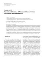
Figure 1: Flow chart of the proposed object-based video analysis framework.
by color and motion segmentation, respectively. Next, a par-
ticle filter tracks the objects over time and compensates for
missing or false detections. The detections, when available,
influence the proposal distribution and the updating of the
target color model (see Figure 1). We evaluate the proposed
framework on the standard datasets CLEAR [11], AMI [12],
and PETS 2001 [13].
The paper is organized as follows. Section 2 introduces
face and people detection and evidence fusion. The integra-
tion of detections in particle filtering and track management
issues are described in Section 3. Section 4 introduces the
performance measures. Section 5 presents the experimental
results. Finally, in Section 6 we draw the conclusions.
2. DETECTING HUMANS AND FACES
2.1. Classifying object categories
The a priori knowledge about object categories to be discov-
ered in a video is incorporated through the training of an
object detector. The validity of the proposed framework is
independent of the chosen detector, and here we use two dif-
ferent detectors to demonstrate the feasibility and generality
of the proposed framework.
In particular, to detect faces and people, we use an Ad-
aboost feature classifier based on a set of Haar-wavelet-like
features (see [14, 15]). These features are computed on the
integral image I(x, y), defined as I(x, y)

=

x
i
=1

y
j
=1
I(i, j),
where I(i, j) represents the original image intensity. The
Haar features are differences between sums of all pixels
within subwindows in the original image. Therefore, in the
integral image, they are calculated as simple differences be-
(a) (b) (c) (d) (e) (f) (g)
(h) (i) (j) (k) (l) (m) (n) (o)
Edge features Center-surround features
Line features
Figure 2: Haar features used for classification. (a–e) edge features;
(f-g) center-surround features; (h–o) line features.
tween the top-left and the bottom-right corners of the corre-
sponding subwindows.
For face detection, we use a trained classifier [16]for
frontal, left, and right profile faces, with the 14 features
shown in Figure 2 (see ((a)–(d), (f)–(o))). The edge feature
shown in Figure 2(e) is used to model tilted edges, such as
shoulders, and it is therefore not suitable for modeling faces.
For people detection, the training was performed using
the 13 features shown in Figure 2 (see ((a)–(e), (h)–(o)))
[15]. We used n

t
= n
+
t
+ n
−
t
= 4285 training samples, with
n
+
t
= 2543 positive 10 × 24 pixel samples selected from the
CLEAR dataset (see Figure 3)andn
−
t
= 1742 negative sam-
ples with different resolutions. Since there is one weak clas-
sifier for each distinct feature combination, effectively there
are 2543
×13 = 33059 weak classifiers that, after training, are
organized in 20 layers. Note that the features in Figure 2 (see
Stefan Karlsson et al. 3
Figure 3: Subset of positive samples used for training the person
detector.
((c), (d), (g), (l)–(o))) are computed on the integral image
rotated by 45
◦
[17].
Let us denote the object classification result with


O
c
t
(x, y, w, h, n), where c denotes the object class (we will use
the subscript f for faces and p for people), n
= 1, , N
c
is
the number of detected objects for class c at time t,(x, y)is
the center of the object, and w and h are its width and height,
respectively.
2.2. Low-level segmentation
Low-level segmentation provides a reliability cue for each
detection. We use skin color segmentation and motion seg-
mentation to support face and person categorization, respec-
tively.
Skin color segmentation is based on a nonlinear transfor-
mation of the YC
b
C
r
color space [18], which results in a two-
dimensional ad hoc chromaticity plane C

b
C

r
. As this trans-
formation is degenerate for gray pixels, RGB values with re-

spect to the conditions 0.975 <R/Band G/B < 1.025 are
discarded. To distinguish skin pixels in the C

b
C

r
plane, an
ellipse encircling skin chromaticity is defined as
x
2
a
2
+
y
2
b
2
= 1, (1)
with

x
y

=

cos θ sin θ
− sin θ cos θ

C


b
− c
x
C

r
− c
y

. (2)
We sampled skin chromaticity from the CLEAR dataset and
computed the values c
x
= 110, c
y
= 152, a = 25, b = 15, and
θ
= 2.53, which are comparable to those in [18]. An example
of skin color segmentation is shown in Figure 4(d).
Motion segmentation is performed using a statistical color
change detector [19]. The detector assumes that a reference
image is available, either because an image without objects
can be taken or because of the use of an adaptive background
algorithm [20, 21]. An example of motion segmentation re-
sults is presented in Figure 4(b).
Let us denote the segmentation mask as S
c
t
(i, j), where

i
= 1, , W and j = 1, , H represent the pixel position,
with W and H representing the image width and height, re-
spectively.
(a) (b)
(c) (d)
Figure 4: Sample segmentation results on CLEAR test sequences.
(a) Outdoor test sequence and (b) corresponding motion segmen-
tation result. (c) Indoor test sequence and (d) corresponding color
segmentation result.
(a) (b)
(c) (d)
Figure 5: Sample person and face detection results. (a) Person de-
tection using the classifier only; (b) filtered detections after evidence
fusion. (c) Face detection using the classifier only; (d) filtered detec-
tions after evidence fusion.
2.3. Evidence fusion
Segmentation results are used to remove false positive detec-
tions. A detection

O
c
t
(x
d
, y
d
, w
d
, h

d
, n) is accepted if



O
c
t

x
d
, y
d
, w
d
, h
d
, n

∩
S
c
t
(i, j)





O

c
t

x
d
, y
d
, w
d
, h
d
, n



>λ
c
,(3)
where
|·| is the cardinality of a set and λ
c
is the minimum
number of segmented pixels used to accept a detected area.
For color segmentation λ
f
= 0.1, whereas for motion segmen-
tation λ
p
= 0.2. The values of these thresholds depend on the
fact that detections may contain background areas (for peo-

ple) or hair regions (for faces). Figure 5 shows two examples
of detection results prior to and after evidence fusion.
4 EURASIP Journal on Image and Video Processing
The resulting object detections are then used to initialize
the object tracker as well as to solve track management issues,
as discussed in the next section.
3. GENERATING TRAJECTORIES
3.1. The tracker
Tracking estimates the state of an object in subsequent
frames. We use a particle filter tracker as it can deal with non-
Gaussian multimodal distributions [5, 22].
Let us represent the target state as x
t
= [x, y, w, h]. The
posterior pdf of a target location in the state space is defined
as a sum of Dirac deltas centered around the particles, with
weights ω
n
t
:
p

x
t
| z
1:t

≈
N
s


n=1
ω
n
t
δ

x
t
− x
n
t

,(4)
where x
n
t
is the state of the nth particle in frame t, z
1:t
are
the measurements from time 1 to time t,andN
s
is the total
number of particles. The state transition p(x
n
t
| x
n
t
−1

)isa
zero-order motion model defined as x
t
= x
t−1
+ N (x
t−1
, σ),
where N (x
t−1
, σ) is a Gaussian noise centered in the previous
state with variance σ. The update of the pdf over time is based
on the recalculation of the weights ω
n
t
:
ω
n
t
∝ ω
n
t
−1
p

z
t
| x
n
t


p

x
n
t
| x
n
t
−1

q

x
n
t
| x
n
t
−1
, z
t

,(5)
where p(z
t
| x
n
t
) is the likelihood of the measurement. Since

we use resampling to avoid the degeneracy of the particles
(i.e., when the weights of all particles except one tend to zero
after few iterations [22]), ω
n
t
−1
= 1/N ∀n and (5) is simpli-
fied to
ω
n
t
∝
p

z
t
| x
n
t

p

x
n
t
| x
n
t
−1


q

x
n
t
| x
n
t
−1
, z
t

. (6)
To compute the likelihood p(z
t
| x
n
t
), we use a color his-
togram φ
M
= [ϕ
M
1,1,1
, , ϕ
M
RGB
] as object model [5, 6], where
R, G,andB are the number of bins in each color channel.
The color difference between the model M and a particle p,

d
J
(φ
M
, φ
p
), is based on the Jeffrey divergence [23]. The like-
lihood is finally estimated as
p

z
t
| x
n
t

=
1

2πσ
l
e
d
J
(φ
M
,φ
p
)
2

/2σ
2
l
. (7)
3.2. Particle propagation
Instead of using the transition prior only, we include ob-
ject detections, when available, in the proposal distribution:
a fraction of the particles is spread around the previous state
according to the motion model, whereas the rest are spread
around the detections. For this reason, each detection has to
be linked to the closest state. This association is established
with a gated nearest neighborhood filter, which selects the
detection O
c
t
(x
d
, y
d
, w
d
, h
d
, n) closest to the state x
t
if it is in
its proximity. The proximity conditions are


x

d
− x
tr


<δ
c

w
tr
+ η
c
h
tr

,


y
d
− y
tr


<δ
c

η
c
w

tr
+ h
tr

,

1 − γ
c

w
tr
<w
d
<

1+γ
c

w
tr
,

1 − γ
c

h
tr
<h
d
<


1+γ
c

h
tr
,
(8)
where (x
tr
, y
tr
) is the center, w
tr
and h
tr
are the width and
height of the ellipse representing the object, and η
f
= 1,
η
p
= 0, δ
f
= γ
p
= 0.25, δ
p
= γ
f

= 0.5 are determined
experimentally. The association is incorporated in (9)[5]as
q

x
t
| x
t−1
, z
t

=
α
c
q
d

x
t
| z
t

+

1 − α
c

p

x

t
| x
t−1

,(9)
where α
c
is the fraction of particles spread around the detec-
tion in the state space and q
d
(x
t
| z
t
) is a Gaussian around
the associated detection. If the proximity conditions are not
satisfied, a new candidate track is initialized and α
c
= 0. In
such a case, (9)reducestoq(x
t
| x
t−1
, z
t
) = p(x
t
| x
t−1
),

whereas (6)reducestoω
n
t
∝ p(z
t
| x
n
t
).
3.3. Model update
Object detections are also used to online update the object
model M. This update aims to avoid track drifting when the
object appearance varies due to changes in illumination, size,
or pose. The color histogram is updated according to
ϕ
M
r,g,b
(t) = β
c
ϕ
d
r,g,b
(t)+

1 − β
c

ϕ
M
r,g,b

(t − 1), (10)
where r
= 1, ,R, g = 1, , G, b = 1, , B,andβ
c
is the
update factor. Note that the histogram is only updated when
there is an associated detection in order to prevent back-
ground pixels from becoming a part of the model M.
3.4. Track management issues
Unlike [5], where tracks are initiated with a single detection,
we integrate information coming from the detector and the
tracker processes to deal with track initiation and termina-
tion issues. A detection O
c
t
(x, y, w, h, n) that is not associated
with a track is considered as a candidate for track initializa-
tion. Tracking is started in sleeping mode.Toswitchatrack
from sleeping to active mode, N
i
detections are accumulated
in subsequent frames. The value of N
i
depends on frequency
of the detections:
N
i
= min

3

2 − 1/f
f ,9

, (11)
where f is the frequency of detections and f
= 9/20 is the
minimum frequency. If there are not a sufficient number of
successive detections, then the track is discarded.
Atrackisterminated if the low-level segmentation results
do not provide enough evidence for the presence of an object:



X
c
t

x
d
, y
d
, w
d
, h
d
, n

∩
S
c

t
(i, j)





X
c
t

x
d
, y
d
, w
d
, h
d
, n



<λ
c
, (12)
Stefan Karlsson et al. 5
(a) (b)
Figure 6: Example of using track management rules for sequence
S3, frame 270. (a) Without track management, the tracked ellipses

degenerate. (b) With track management, the tracked ellipses cor-
rectly estimate the face areas.
with λ
p
= 0.2andλ
f
= 0.1. Moreover, a person track is
terminated if N
t
= 25 subsequent frames without an asso-
ciated detection. A face track is terminated when the color
histogram of the object changes drastically; that is, the Jef-
frey divergence d
J
between the current target and the model
is larger than a threshold D. A cut-off distance of D
= 0.15
was found appropriate. Also, we terminate the tracks that de-
viate more than 3σ from the average face size, learnt on the
first 300 tracked faces. Finally, faces whose ratio is w/h > 1.5
are considered unlikely and therefore removed. An example
of performance improvements achieved with the proposed
initialization and termination rules is shown in Figure 6.
3.5. Postprocessing
Track verification is performed to remove false tracks in a
postprocessing stage. False tracks are generally initiated by
repeated multiple detections on the same object. To remove
these tracks, a score is computed for each overlapping track:
s
n

t
= (0.6N
f
)/50 + 0.4fr
d
,wheres
n
t
is the score for track n
at time t, N
f
is the number of frames tracked in a 50-frame
window, and fr
d
is the frequency of detection. The weights on
N
f
(0.6) and fr
d
(0.4) favor tracks with a long history against
new ones with a high frequency. Finally, tracks shorter than
15 frames are likely to be cluttered and therefore removed.
4. PERFORMANCE MEASURES
To quantitatively evaluate the performance of the proposed
framework, two groups of measures are used, namely, detec-
tion and tracking performance measures. We chose as detec-
tion measures precision P and recall R, which are designed to
quantify the ability of an algorithm to identify true targets in
a video, as opposed to false detections and missed detections.
These measures are commonly used to evaluate the perfor-

mance of database retrieval algorithms and are defined as
P
=
TP
TP + FP
,
R
=
TP
TP + FN
,
(13)
where TP is the number of true positives,FPisthenumberof
false positives, and FN is the number of fals e negatives.
Table 1: Brief information about the datasets.
Dataset Seq. Sequence name Task Frames
AMI
S1 EN2001b.Closeup1 face 100–600
S2 EN2001b.Closeup4 face 1–500
S3 IS1003c.L face 1–500
S4 IS1004a.R face 250–750
CLEAR
S5 PVTRA102a09 people 500–3001
S6 PVTRA102a10 people 3007–5701
S7 PVTRA102a11 people 1–500
S8 PVTRA102a12 people 1000–1500
PETS S9 PETS1SEG people 1–500
The tracking performance measures quantify the accu-
racy of the estimated object size (d
D

) and the accuracy of
the estimated object position (d
Dist
). The measure d
D
quan-
tifies the overlap between the ground truth and the estimated
targets, and it is defined as
d
D
= 1 −

N
fn
n=1

N
fr
t=1

2


G
(t)
n
∩ D
(t)
n



/


G
(t)
n
+ D
(t)
n




N
fr
u=1
N
u
fn
, (14)
where G
(t)
n
denotes the ground truth for track n at time t,
D
(t)
n
is the corresponding estimated target, N
fn

is the number
of matched objects in the ground truth and the tracked ob-
jects in a frame, N
fr
is the total number of frames, and N
u
fr
is
the total number of matched objects in the entire sequence.
The measure d
Dist
is the distance between the centers of the
estimated tracked object and the ground truth, normalized
by the size of the ground truth:
d
Dist
=

N
fn
n=1

N
fr
t=1


(x
d
− x

g
)/w
g

2
+

(y
d
− y
g
)/h
g

2

N
fr
u=1
N
u
fn
,
(15)
where (x
d
, y
d
)and(x
g

, y
g
) are the centers of the tracked ob-
ject and the ground truth, and w
g
and h
g
are the width and
height of the corresponding ground truth object.
5. EXPERIMENTAL RESULTS
We demonstrate the proposed framework on three stan-
dard datasets, namely, CLEAR, AMI, and PETS 2001. These
datasets include indoor and outdoor scenarios for a total of
8700 frames (see Ta bl e 1 ).
The same set of parameters is used for motion segmen-
tation and for the tracker in all the experiments. For the sta-
tistical change detector, the noise variance is σ
= 1.8and
the kernel size is k
= 3. The particle filter uses 150 particles
per object, with a transition factor of 12 pixels per frame.
For the likelihood (7), α
l
= 0.068. For faces, α
f
= 0.9and
β
f
= 0.35, and for people, α
p

= 0.25 and β
p
= 0.1. These
values have been found appropriate after extensive testing.
The histogram for the color model and the likelihood is uni-
formly quantized with 10
× 10 × 10 bins in the RGB space.
We compare the proposed approach that integrates de-
tections and particle filtering (referred to as PFI) with the
6 EURASIP Journal on Image and Video Processing
Table 2: Comparison of tracking performance (means and stan-
dard deviations for 8 runs).
Faces
Seq. PFI PF NN
S1
d
D
(σ
d
D
) 0.24(0.02) 0.25(0.03) 0.27
d
Dist
(σ
d
Dist
) 0.10(0.004) 0.14(0.02) 0.10
P(σ
P
) 0.76(0.06) 0.70(0.03) 0.70

R(σ
R
) 1.00(0) 0.98(0.03) 1
S2
d
D
(σ
d
D
) 0.28(0.01) 0.34(0.01) 0.28
d
Dist
(σ
d
Dist
) 0.13(0.005) 0.24(0.01) 0.12
P(σ
P
) 0.95(0.01) 0.92(0.03) 0.94
R(σ
R
) 0.96(0.01) 0.89(0.01) 0.94
S3
d
D
(σ
d
D
) 0.27(0.03) 0.39(0.01) 0.32
d

Dist
(σ
d
Dist
) 0.13(0.02) 0.21(0.02) 0.16
P(σ
P
) 0.52(0.03) 0.38(0.02) 0.47
R(σ
R
) 0.73(0.03) 0.74(0.02) 0.72
S4
d
D
(σ
d
D
) 0.38(0.03) 0.49(0.03) 0.26
d
Dist
(σ
d
Dist
) 0.26(0.03) 0.41(0.04) 0.17
P(σ
P
) 0.66(0.08) 0.52(0.04) 0.60
R(σ
R
) 0.69(0.06) 0.48(0.05) 0.29

People
Seq. PFI PF NN
S5
d
D
(σ
d
D
) 0.25(0.02) 0.26(0.01) 0.24
d
Dist
(σ
d
Dist
) 0.18(0.01) 0.17(0.02) 0.19
P(σ
P
) 0.78(0.02) 0.78(0.01) 0.80
R(σ
R
) 0.90(0.02) 0.92(0.03) 0.82
S6
d
D
(σ
d
D
) 0.25(0.05) 0.35(0.03) 0.21
d
Dist

(σ
d
Dist
) 0.16(0.03) 0.22(0.02) 0.13
P(σ
P
) 0.23(0.04) 0.22(0) 0.26
R(σ
R
) 0.55(0.08) 0.59(0.11) 0.62
S7
d
D
(σ
d
D
) 0.36(0.04) 0.36(0.01) 0.31
d
Dist
(σ
d
Dist
) 0.21(0.02) 0.24(0.02) 0.17
P(σ
P
) 0.74(0.04) 0.70(0.02) 0.81
R(σ
R
) 0.84(0.01) 0.84(0.01) 0.84
S8

d
D
(σ
d
D
) 0.34(0.03) 0.37(0.04) 0.35
d
Dist
(σ
d
Dist
) 0.21(0.02) 0.21(0.03) 0.21
P(σ
P
) 0.59(0.02) 0.57(0.03) 0.60
R(σ
R
) 0.67(0.02) 0.65(0.04) 0.61
particle filtering alone (referred to as PF). To offer a fair com-
parison, in both cases the initialization and termination rules
presented in Section 3.4 are used. We also compare PFI with
the nearest neighborhood filter (NN). The measurements
used for evaluation are the mean (
d
D
, d
Dist
, R,andP)and
the corresponding standard deviations on 8 runs of the per-
formance measures presented in Section 4 (see Ta bl e 2).

The comparison of PFI and PF for faces shows that
d
D
and d
Dist
scores are smaller for all face sequences indicating
better correspondence between track ellipses and the ground
truth. Further,
R and P are larger for the same sequences,
except for one
R score. Figure 9 shows sample results of peo-
ple and face tracking, and their framewise
d
D
scores are il-
lustrated in Figure 8.InFigure 8 (row 1), the quality of PFI
(a) (b)
(c) (d)
Figure 7: Comparison of tracking results between NN (green) and
PFI (blue). (a) Sequence S2 and (b) Sequence S4: the NN algorithm
fails when there is low frequency of detections. (c) Sequence S6 and
(d) Sequence S7: the NN filter produces jagged trajectories.
0
0.1
0.2
0.3
0.4
0.5
0.6
d

D
S3
248 258 268 278 288 298 308 318 328 338
Frames
0
0.1
0.2
0.3
0.4
0.5
0.6
d
D
S2
17 22 27 32 37 42 47 52 57 62 67
Frames
0
0.1
0.2
0.3
0.4
0.5
0.6
d
D
S5
2500 2550 2600 2650 2700 2750 2800
Frames
0
0.1

0.2
0.3
0.4
0.5
0.6
d
D
S5
2500 2550 2600 2650 2700 2750 2800
Frames
PFI
PF
Figure 8: Performance comparison of face tracks (sequence S3 and
S2) and people tracks (sequence S5) for PF and PFI.
Stefan Karlsson et al. 7
(a) (b)
(c) (d)
Figure 9: Comparison of tracking results with PF (green) and PFI (blue). (a)–(b) Sequence S5; (c) sequence S2; (d) sequence S3.
(a)
0
50
100
150
200
250
300
350
400
450
500

Time (t) (seconds)
200
100
0
Height (pixels)
0
50
100 150
200
250
300
350
Width (pixels)
300
200
100
0
Width (pixels)
250
200
150
100
50
0
Height (pixels)
200
300
400
500
600

700
Time (t) (seconds)
(b)
(c)
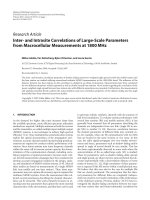
Figure 10: Example of trajectory-based video description and object prototypes. (a) Resulting tracks superimposed on the images. (b)
Evolution of the tracks over time. (c) Automatically generated key-objects for frontal, left, and right profile faces.
8 EURASIP Journal on Image and Video Processing
results improves more quickly than those of PF. The aver-
age
d
D
for PFI is 0.17 and for PF is 0.33, and in Figure 8
(row 2), the average for PFI is 0.24 and the average for PF
is 0.31. In Figure 8, rows 3 and 4, are the human tracking ex-
amples with average of 0.22 and 0.12 for PFI and average of
0.30 and 0.15 for PF, respectively. The lower average values of
d
D
in all these cases show improved performance of PFI over
PF.
The comparison between PFI and NN for faces shows
that the
d
D
and d
Dist
scores are better for sequences S1 and
S3, similar for sequence S2, whereas these scores indicate bet-
ter performance of the NN tracker for S4, but with lower
R

and
P scores. The reason is that in S4 the NN tracker fails
to track in parts of the sequence with very low frequency of
detections, whereas the particle filter succeeds in tracking in
these regions (see Figure 7). For people tracking, the scores
are similar for S5 and S8, whereas NN is better for S6 and
S7 because sometimes detections that are larger than the per-
son dominate in frequency, and PFI will filter out the cor-
rectly sized detections (which are instead taken into account
by NN).
To c o n c l u d e , Figure 10 shows an example of trajectory-
based video description using spatiotemporal object
trajectories of two faces and the corresponding object
prototypes (frontal and profile faces). Only the true tracks
are computed by the proposed algorithm and false de-
tections and associated tracks are filtered out using skin
color segmentation and postprocessing. Videos results are
available at />detrack.html.
6. CONCLUSIONS
We presented a general video analysis framework for detect-
ing and tracking object categories and demonstrated it on
people and faces. Video results and quantitative measure-
ments show that the proposed integration of detections with
particle filtering improves the robustness of the state estima-
tion of the targets.
The proposed framework is general, and classifiers of
other body parts and other object types can be incorporated
without changing the overall structure of the algorithm. Us-
ing additional object detectors, a complete story line of a
video based on specific object categories and their trajec-

tories could be produced, describing interactions and other
important events. Moreover, the video could be annotated
semantically with identity information of the appearing per-
sons by adding a face recognition module [24].
Our current work includes improving the performance
of the human detector by using a larger training database and
refining the bounding boxes of the detection using edges and
motion segmentation results.
ACKNOWLEDGMENT
The authors acknowledge the support of the UK Engineer-
ing and Physical Sciences Research Council (EPSRC), under
Grant no. EP/D033772/1.
REFERENCES
[1] A. Cavallaro and S. Winkler, “Perceptual semantics,” in Digital
Multimedia Perception and Design, G. Ghinea and S. Y. Chen,
Eds., Idea Group, Toronto, Canada, April 2006.
[2] S. Gangaputra and D. Geman, “A unified stochastic model for
detecting and tracking faces,” in Proceedings of the 2nd Cana-
dian Conference on Computer and Robot Vision, pp. 306–313,
Victoria, BC, Canada, May 2005.
[3] B. Wu and R. Nevatia, “Detection and tracking of multiple,
partially occluded humans by Bayesian combination of edgelet
based part detectors,” International Journal of Computer Vi-
sion, vol. 75, no. 2, pp. 247–266, 2007.
[4] R.vanderMerwe,ADoucet,J.F.G.deFreitas,andE.Wan,
“The unscented particle filter,” in Advances in Neural Informa-
tion Processing Systems 14 (NIPS ’01), vol. 8, pp. 351–357, Van-
couver, BC, Canada, December 2001.
[5] K. Okuma, A. Taleghani, N. de Freitas, J. J. Little, and D.
G. Lowe, “A boosted particle filter: multitarget detection and

tracking,” in Proceedings of the 8th European Conference on
Computer Vision (ECCV ’04), vol. 1, pp. 28–39, Prague, Czech
Republic, May 2004.
[6] X. Xu and B. Li, “Head tracking using particle filter with in-
tensity gradient and color histogram,” in Proceedings of IEEE
International Conference on Multimedia and Expo (ICME ’05),
vol. 2005, pp. 888–891, Amsterdam, The Netherlands, July
2005.
[7] S. McKenna and S. Gong, “Tracking faces,” in Proceedings of
the 2nd International Conference on Automatic Face and Ges-
ture Recognition, pp. 271–276, Killington, VT, USA, October
1996.
[8] P. Withagen, K. Schutte, and F. Groen, “Object detection and
tracking using a likelihood based approach,” in Proceedings of
the Advanced School for Computing and Imaging Conference,
vol. 2, pp. 248–253, Lochem, Netherlands, June 2002.
[9] M.G.S.BrunoandJ.M.F.Moura,“IntegrationofBayesde-
tection and target tracking in real clutter image sequences,” in
Proceedings of IEEE International Radar Conference, pp. 234–
238, Atlanta, GA, USA, May 2001.
[10] P. Willett, R. Niu, and Y. Bar-Shalom, “Integration of Bayes de-
tection with target tracking,” IEEE Transactions on Signal Pro-
cessing, vol. 49, no. 1, pp. 17–29, 2001.
[11] R. Kasturi, “Performance evaluation protocol for face, person
and vehicle detection & tracking in video analysis and content
extraction (VACE-II),” Computer Science & Engineering
University of South Florida, Tampa, FL, USA, January 2006,
/>Protocol
v5.pdf.
[12] July 2007.

[13] />July 2007.
[14] P. Viola and M. Jones, “Rapid object detection using a boosted
cascade of simple features,” in Proceedings of IEEE Computer
SocietyConferenceonComputerVisionandPatternRecogni-
tion, vol. 1, pp. 511–518, Kauai, HI, USA, December 2001.
[15]P.Viola,M.J.Jones,andD.Snow,“Detectingpedestrians
using patterns of motion and appearance,” in Proceedings of
IEEE International Conference on Computer Vision (ICCV ’03),
vol. 2, pp. 734–741, Nice, France, October 2003.
[16] G. Bradski, A. Kaehler, and V. Pisarevsky, “Learning-based
computer vision with Intel’s open source computer vision li-
brary,” Intel Technology Journal, vol. 9, pp. 119–130, 2005.
[17] R. Lienhart and J. Maydt, “An extended set of Haar-like fea-
tures for rapid object detection,” in Proceedings of International
Stefan Karlsson et al. 9
Conference on Image Processing (ICIP ’02), vol. 1, pp. 900–903,
Rochester, NY, USA, September 2002.
[18] R L.Hsu,M.Abdel-Mottaleb,andA.K.Jain,“Facedetection
in color images,” IEEE Transaction on Pattern Analysis Machine
Intelligence, vol. 24, no. 5, pp. 696–706, 2002.
[19] A. Cavallaro and T. Ebrahimi, “Interaction between high-level
and low-level image analysis for semantic video object extrac-
tion,” EURASIP Journal on Applied Signal Processing, vol. 2004,
no. 6, pp. 786–797, 2004.
[20] R. J. Radke, S. Andra, O. Al-Kofahi, and B. Roysam, “Image
change detection algorithms: a systematic survey,” IEEE Trans-
actions on Image Processing, vol. 14, no. 3, pp. 294–307, 2005.
[21] C. Stauffer and W. E. L. Grimson, “Learning patterns of ac-
tivity using real-time tracking,” IEEE Transactions on Pattern
Analysis and Machine Intelligence, vol. 22, no. 8, pp. 747–757,

2000.
[22] M. S. Arulampalam, S. Maskell, N. Gordon, and T. Clapp, “A
tutorial on particle filters for online nonlinear/non-gaussian
bayesian tracking,” IEEE Transactions on Signal Processing,
vol. 50, no. 2, pp. 174–188, 2002.
[23] Y. Rubner, J. Puzicha, C. Tomasi, and J. M. Buhmann, “Em-
pirical evaluation of dissimilarity measures for color and tex-
ture,” in Proceedings of the IEEE Computer Society Conference
on Computer Vision and Patte rn Recognition (CVPR ’01), vol. 2,
pp. 25–43, Kauai, HI, USA, December 2001.
[24] J. Ruiz-del-Solar and P. Navarrete, “Eigenspace-based face
recognition: a comparative study of different approaches,”
IEEE Transactions on Systems, Man and Cybernetics Part C,
vol. 35, no. 3, pp. 315–325, 2005.