Báo cáo hóa học: " Research Article Efficient Reduction of Access Latency through Object Correlations in Virtual Environments" pdf

Hindawi Publishing Corporation
EURASIP Journal on Advances in Signal Processing
Volume 2007, Article ID 10289, 19 pages
doi:10.1155/2007/10289
Research Article
Efficient Reduction of Access Latency through Object
Correlations in Virtual Environments
Shao-Shin Hung and Damon Shing-Min Liu
Department of Computer Science and Information Engineering, National Chung Cheng University, Chia-Yi 62107, Taiwan
Received 1 September 2006; Accepted 22 February 2007
Recommended by Ebroul Izquierdo
Object correlations are common semantic patterns in virtual environments. They can be exploited to improve the effectiveness of
storage caching, prefetching, data layout, and disk scheduling. However, we have little approaches for discovering object correla-
tions in VE to improve the per formance of storage systems. Being an interactive feedback-driven paradigm, it is critical that the
user receives responses to his navigation requests with little or no time lag. Therefore, we propose a class of view-based projection-
generation method for mining various frequent sequential traversal patterns in the virtual environments. The frequent sequential
traversal patterns are used to predict the user navigation behavior and, through clustering scheme, help to reduce disk access
time with proper patterns placement into disk blocks. Finally, the effectiveness of these schemes is shown through simulation to
demonstrate how these proposed techniques not only significantly cut down disk access time, but also enhance the accuracy of
data prefetching.
Copyright © 2007 S S. Hung and D. S M. Liu. This is an open access article distributed under the Creative Commons Attribution
License, which permits unrestricted use, distribution, and reproduction in any medium, provided the original work is properly
cited.
1. INTRODUCTION
With ever-increasing demands for storing very large vol-
umes of data for applications such as telemedicine, online
computer entertainment systems, and other large multime-
dia repositories, large amounts of live data are being stored
on the storage systems. Random accesses to data stored on
storage system can suffer unacceptable delays as media are
swapped on drives. The need for swapping media is dictated

by the placement of data. Judicious placement of data on the
storage media is therefore critical, and can significantly af-
fect the overall performance of the storage system. One pri-
mary factor is the placement of data for storage system [1, 2].
The placement of data for sp ecific domains such as multi-
dimensional arrays [1], relational databases [3], and satellite
images [4] has been addressed earlier. Research on the stor-
age placement in a more general setting has been addressed
under the assumption that data objects are accessed indepen-
dently [1]. This assumption is rarely valid in practice-data
objects typically related (correlated)andthisisreflectedin
the access of the data [5].
On the other side, with the advent of advanced com-
puter hardware and software technologies, virtual environ-
ments (VE) are becoming larger and more complicated. To
satisfy the growing demand for fidelity, there is a need for
interactive and intelligent schemes that assist and enable ef-
fective and efficient storage management. Unfortunately, it
is not an easy task to exploit the intelligence in storage sys-
tems. File access patterns are not random, they are driven
by applications and user behaviors [6]. This fact, coupled
with the growing performance bottleneck of computer stor-
age systems, has resulted in a significant amount of research
improving file systems behavior through predicting future ac-
cess objects. Latency is an ever-increasing component of data
access cost, which in turn is usually the bottleneck for mod-
ern high performance systems [7]. For this reason, accurate
access prediction mechanism is very desirable for data stor-
age system. In such a case, VEs do not consider the problem
of access times of objects in the storage systems. They are al-

ways simply concerned about how to display the object in
the next frame. As a result, the VE can only manage data at
the rendering and other related levels without knowing any
semantic information such as semantic correlations between
data. Therefore, much previous work had to rely on simple
patterns such as level-of-detail (LOD) [8], view-dependent
simplification [9], out-of-core simplification [8], bounding
volume hierarchies (BVHs) [10–12], and occlusion culling
to improve system performance, without fully exploiting its
2 EURASIP Journal on Advances in Signal Processing
1
2
3
4
5
6
7
8
9
10
11
12
13
14
15
16
17
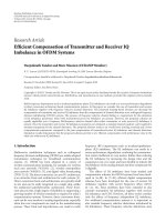
Figure 1: The circle shows how many objects the view contains, and
arrow line represents view sequence when user traverses the path.
intelligence. This motivates a more powerful analysis tool to

discover more complex patterns, especially semantic patterns,
in storage systems. Therefore, the aim of our work is to de-
crease this latency through intelligent organization of the ac-
cessed objects and enabling the clients to perform predictive
prefetching.
In this paper, we consider the problem and solve this us-
ing data mining techniques [13, 14]. Clearly, when users tra-
verse in a virtual environment, some potential semantic char-
acteristics will emerge on their traversal paths. If we collect
the users’ traversal paths, mine and extract some kind of in-
formation of them, such meaningful semantic information
can help to improve the performance of the interactive VE.
For example, we can reconstruct the placement order of the
objects of 3D model in disk according to the common sec-
tion of users’ path. Exploring these correlations is very useful
for improving the effectiveness of storage caching, prefetch-
ing, data layout, and disk scheduling. Consider the scenario
in Figure 1, the rectangle represents an object, and the circle
represents a view associated with a certain position. Due to
spatial locality, we may take objects 1 and 3 into the same disk
block. However, if the circular view does exist in the path, the
mining algorithm will give us different information for such
situation. The mining algorithm may suggest to collect ob-
ject 1, 4, and 7 into the same disk block, instead of object 1
and 3, because of the semantic correlation.
This paper proposes VSPM (viewed-based sequential pat-
tern mining), a method which applies a data mining tech-
nique called frequent sequential pattern mining to discover
object correlations in VE. Specially, we have modified several
recently proposed data mining algorithms called FreeSpan

[15]andPrefixSpan [16] to find object correlations in sev-
eral traversal traces collected in real systems. To the best of
our knowledge, VSPM is the first approach to infer object
correlations in a VE. Furthermore, VSPM is more scalable
and space-efficient than previous approaches. It runs reason-
ably fast with reasonable space overhead, indicating that it is
a practical tool for dynamically inferring correlations in a VE.
Besides, we have also proposed a clustering method to clus-
ter similar patterns for reducing the access time. According to
some similarity functions, or other measurements, clustering
aims to partition a set of objects into several groups such that
“similar” objects are in the same group. It will make similar
objects much closer to be accessed in one time. This results
in less access times and much better performance. In order to
evaluate the validity of clustering, the two criteria, cluste r co-
hesion and inter-cluster similarity, were presented. Moreover,
we also have evaluated the benefits of objec t correlation-
directed prefetching and disk data layout using the synthetic
datasets [17] and the real system workloads. Compared to
the base case, under the number of files accessed condition,
this scheme reduces the average number of accessed files by
33.3% ((4
− 3)/3 = 0.333 is shown in Figure 12) to 2.625
((27
− 8)/8 = 2.625 is shown in Figure 12). Compared to the
sequential prefetching scheme, it also reduces the average re-
sponse time by 35.6% ((624
− 460)/460 = 0.356 is shown in
Figure 13) to 1.249 ((4983
− 2215)/2215 = 1.249 is shown in

Figure 13).
The rest of this paper is organized as follows. Related
works are given in Section 2.InSection 3,wedescribeour
problem formulation. The system architecture is suggested in
Section 4. The suggested mining and clustering mechanisms
are explained with illustrative examples shown in Section 5.
Section 6 presents our experiment results. Finally, we sum-
marize our current results with suggestions for future re-
search in Section 7.
2. RELATED WORKS
In this section, we summarize related work in the area of vir-
tual environments, sequential pattern mining, and pattern
clustering.
2.1. Virtual environments methods
Despite the use of advanced graphics hardware, real-time
navigation in high complex virtual environments is still a
challenging problem because the demands on image qual-
ity and details increase exceptionally fast. The navigation in
virtual environments consists of many different detailed ob-
jects, for example, of CAD data that cannot all be stored in
main memory but only on hard disk. In other words, pro-
viding efficient access to huge VR datasets has attracted a lot
of attention. A great deal of work has been done in related
visualization algorithms. These algorithms can be classified
into several categories according to their used data structures,
data management systems, storage ordering, or optimizing
file systems using techniques like prefetching and caching.
2.1.1. Chunking
Sarawagi and Stonebraker [18] describe chunking, which
groups spatially adjacent data elements into n-dimensional

chunks which are then used as basic I/O unit, making ac-
cess to multidimensional data and order of magnitude faster.
They also arrange the storage order of these chunks to min-
imize sought distance dur ing access. Related chunking algo-
rithms [19] reorganize their data according to the expected
S S. Hung and D. S M. Liu 3
query type, and the likelihood that data values will be ac-
cessed together. However, for extremely large datasets, it is
impractical to make a copy of the dataset for each expected
access pattern [20].
2.1.2. Prefetching and caching
Prefetching has been used by many researchers to hide or
minimize the cost of I/O stalling. Current researches fo-
cus on visibility-based prefetching algorithm for retrieving
out-of-core 3D models and rendering them at interactive
rates [21]. The go al of prefetching through the multithread-
ing mechanism is to have the geometry already in memory
by the time it is needed. But the threads will occupy some
of the main memory and this strategy need well-planned
switching mechanism to handle threads. Especially, for large
datasets in virtual environments, this scheme cannot be scal-
able. Rhodes et al. [22]proposeiterators and threaded pre-
fecthing scheme based on the concept of spatial prefteching
for improvement on I/O performance. Yoon and Manocha
[10] discuss the cache-efficient layout of bounding volume
hierarchies (BVHs) of polygonal models. They also intro-
duce a new probabilistic model to predict the running ac-
cess patterns of a BVH. Since such large BVH-based kd-
trees will be stored in the storage system for access, this
will result in large I/O times. Chisnall et al. [23]present

knowledge-based out-of-core prefetching algorithms with-
out using hard-coded rendering-related logic by utilizing the
access history and patterns dynamically, and adapting their
prefetching strategies accordingly. However, it seems to be
weak for the basis for such knowledge-based out-of-core al-
gorithm of LRU-related schemes. Semantic correlations seem
to lack in this scheme.
2.1.3. Level-of-detail models
An LOD model essentially per mits to obtain different repre-
sentations of an object at different levels of detail, where the
level can also vary over the object. Performance requirements
impose several challenges in the design of system based on
LOD models, where geometric data st ructures play a cen-
tral role. There is a necessary tradeoff between time effi-
ciency and storage costs. And also there is a tradeoff between
generality and flexibility of models on one hand, and opti-
mization of per formance (both in time and storage) on the
other hand. We classify LOD data structures according to the
dimensionality of the basic structural element they repre-
sent into point- [24], triangle- [25], and tetrahedron-based
[26, 27] data structures. Current researches [28, 29]exploit
the feature of on-board video memory to store geometry in-
formation. This strategy significantly reduces the data trans-
fer overhead from sending geometry data over the (AGP) bus
interface from the main memory to the graphics card.
2.1.4. Occlusion culling
Known occlusion culling algorithms [30–32] manage the
polygons in volume-separating data structures, as, for exam-
ple, quad-trees, oct-tree [33–35], and R-trees [36]were pre-
sented. All polygons in a certain 3D-volume bounded by a

box are attached with it. If such a bounding box is not visi-
ble, all attached polygons are also not visible. There are two
different types of occlusion culling algorithms. One is image-
space occlusion culling algorithms: these algorithms test the
visibility of a box with its projection onto the viewing plane.
However, in practice, reading the values appears to be quite
expensive, especially on PC architectures. The other is object-
based occlusion culling algorithms: these algorithms need no
expensive accesses to any buffer, but they often have the dis-
advantage that they depend on occluders that are large or well
chosen in the preprocessing. Furthermore, they obtain only
poor results in virtual environments which consist of many
single noncoherent polygons. Of course there exist some al-
gorithms, for example, see [37], which allow a real-time nav-
igation in complex scenes, but they often have the disadvan-
tages that they only fit for officeroomsorothersimilarar-
chitectural scenes that have a volume-separating structure. A
more precise overview on occlusion culling algorithms can
be found in [38].
In addition, massive model rendering (MMR) system
[39] was the first published system to handle models with
tens of millions of polygons at interactive frame rates. On
the other side, it is desirable to store only the polygons and
not to produce additional data, for example, textures or pre-
filtered points. However, polygons of such highly complex
scenes require a lot of hard disk space so that the additional
data could exceed the available capacities [40
, 41]. To meet
these requirements, an appropriate data structure and an ef-
ficient technique should be developed with the constraints of

memory consumptions.
2.2. Sequential pattern mining methods
Sequential pattern mining was first introduced in [42], which
is described as follows. A sequence database is formed by
a set of data sequences. Each data sequence includes a se-
ries of transactions, ordered by transac tion times. This re-
search aims to find all the subsequences whose ratios of ap-
pearance exceed the minimum support threshold. In other
words, sequential patterns are the most frequently occurring
subsequences in sequences of sets of items. A number of al-
gorithms and techniques have been proposed to deal with
the problem of sequential pattern mining. Many studies have
contributed to the efficient mining of sequential patterns
[15, 16]. Almost all of the previously proposed methods for
mining sequential patterns are apriori-like, that is, based
on the aprioriproperty proposed in association rule min-
ing [15], which states the facts that any super pattern of a
nonfrequent pattern cannot be frequent. The studies [15, 16]
show that the apriori-like sequential pattern mining meth-
ods bear three nontrivial, inherent costs which are indepen-
dent of detailed implementation techniques. First is that the a
priori-like method may generate potentially huge set of can-
didate sequences during the permutations of elements and
repetition of items in a sequence. Second is that multiple
scans of databases are needed for deciding the support of
these candidates. As the length of candidates increases, the
times of scans of databases become worse. Third is that there
4 EURASIP Journal on Advances in Signal Processing
are many difficulties in mining long sequential patterns. Se-
quential pattern mining algorithms, in general, can be cate-

gorized into three classes: (1) apriori-based, horizontal parti-
tion methods, and GSP [43] is one known representative; (2)
apriori-based, vertical partition methods, and SPADE [44]
is one example; (3) projection-based pattern growth method,
such as the famous FreeSpan [16]andPrefixSpan algorithms
[15].
In this study, we develop a new sequential pattern mining
method, called view-based sequential patter n mining. Since
our input data are different from those of traditional data
mining algorithms [45], we make several major modifica-
tions about the idea of pattern-growth method. Its general
idea is to use frequent objects to recursively project sequence
databases into a set of smaller projects database and grow
subsequence fragments in each projected database. This pro-
cess partitions both the database and the set of frequent ob-
jects to be tested, and confines each test being conducted to
the corresponding smaller projected database.
2.3. Pattern clustering methods
Clustering is one of the main tasks in the data mining process
for discovering groups, and identifying interesting distribu-
tions and patterns in the underlying data. The fundamental
clustering problem is to partition a given dataset into groups
(clusters), such that data points in a cluster are more simi-
lar to each other (i.e., intrasimilar property) than points in
different clusters (intersimilar property) [46].
There is a multitude of clustering methods available in
literature, which can be distinguished with respect to its algo-
rithmic properties [47]. First, partition algorithms strive for
a successive improvement of an existing clustering and can
be further classified into examplar-based and commutation-

based approaches. These approaches need information with
regard to expected cluster number k. Representatives are k-
means [47]andk-medoid [48]. Second, hierarchical algo-
rithms create a tree of node subsets by successively merging
(agglomerative approach) or subdividing (divisive approach)
the objects. In order to obtain a unique clustering, a second
step is necessary that prunes this tree at adequate places. Rep-
resentatives are k-nearest-neighbor and linkage [49]. Finally,
density-based algorithms try to separate a similarity graph
into subgraphs of high connectivity values. In the ideal case,
they can determine the cluster number k automatically and
detect clusters of arbitrary shape and size. Representatives
are: DBSCAN and Chameleon [50].
Although there are many clustering algorithms presented
above, they cannot be applied to our dataset directly. The
reasons are as follows [51]. First is that our database is com-
posed of many transactions. There is a finite set of elements,
called items from a common item universe, contained in a
transaction. Every transaction can b e presented in a point-
by-attribute format, by enumerating all items j
, and by asso-
ciating with a transaction the binary attributes that indicate
whether j items belong to a transaction or not. Such repre-
sentation is s parse that two random transactions have ver y
few items in common. Common to this and other examples
of point-by-attribute for mat for transaction data is high di-
mensionality, significant amount to zero values, and small
number of common values between two objects. Conven-
tional clustering methods, based on similarity measures, do
not work well. Since transactional data is important in clus-

tering profiling, web analysis, DNA analysis, and other appli-
cations, different clustering methods founded on the idea of
cooccurrence of transaction data have been developed. They
are usual ly measured by Jaccard coefficient SIM (T
1
, T
2
) =
|
T
1
∩ T
2
|/|T
1
∪ T
2
| [52, 53].
However, there are some drawbacks of the existing meth-
ods. First, they always consider the single item accessed in the
storage systems. They only care about how many I/O times
the item is accessed. On the other side, we pay more atten-
tion to whether we can fetch objects together involved in the
same view as many as possible, this scheme will help to re-
spond to users’ requests more efficiently. Second, existing al-
gorithms for efficient accessing patterns often rely on differ-
ent data structures or heuristic principles (e.g., prefetching
mechanism based on LRU and the like [11, 22, 23, 54]) to
support the prediction on future desired patterns. Whatever
the data structures or schemes were applied, one problem

always happens. If object a and object b are frequently ac-
cessed together, but the locations between them may be far
away, it is possible for us to access them in more than two
or more times. In this case, not only which objects are ac-
cessed frequently, but also how to layout these objects in the
storage system for reducing the access times. Finally, many
existing algorithms used in visualization are closely coupled
with application-specific logic. Since the intelligence or se-
mantic correlations were embedded in the previous process-
ing, they neglect exploiting the valuable information to help
to arrange the data layout in the storage systems. One possi-
ble solution is to propose a framework of data management
based on knowledge to discover the possible promising objects
for future access. Then, we can minimize disk I/O overhead
by clustering those promising objects into the proper data
layout in the storage systems [55, 56].
3. MOTIVATIONS
3.1. Motivations on theoretical foundations
Data mining research deals with finding relationships among
data items and grouping the related items together. The two
basic relationships that are of particular concern to us are
(i) association, where the only knowledge we have is that
the idea items are frequently occurring together, and
when one occurs, it is highly probable that the other
will also occur;
(ii) sequence, where the data items are associated, and in
addition to that, we know the order of occurrence as
well.
Our ideas can be divided into several concerns. First, ob-
ject correlations can be exploited to improve storage system

performance. Correlations can be used to direct prefetching
[46]. For example, if a strong correlation exists between ob-
jects, these two objects can be fetched together from disks
whenever one of them is accessed. The disk read-ahead
S S. Hung and D. S M. Liu 5
optimization is an example of exploiting the simple sequen-
tial block correlations by prefetching subsequent disk blocks
ahead of time. Several studies [46, 57, 58] have shown that
using e ven these simple sequential correlations can signif-
icantly improve the storage system performance. Second, a
storage system can also lay out data in disks according to ob-
ject correlations. For example, an object can be collocated
with its correlated blocks so that they can be fetched together
using just one disk access. This optimization can reduce the
number of disk seeks and rotations, which dominate the av-
erage disk access latency. With correlated-directed disk lay-
outs, the system only needs to pay one-time seek and rota-
tional delay to get multiple blocks that are likely to be ac-
cessed soon. Previous studies [55, 56] have shown promising
results in allocating correlated file blocks on the same track
to avoid track-switching costs.
As the concept of sequence is based on associations,
we first briefly introduce the issue of finding associations.
The formal definition of the problem of finding associa-
tion rules among items is provided by [59]asfollows.Let
I
= i
1
, i
2

, , i
n
be a set of literals, called items, and let D be
a set of transactions such that for all T
∈ D, T ⊆ I.Atrans-
action T contains a set of items X if X
⊆ T.Anassociation
rule is denoted by an implication of the form X
⇒ Y,where
X
⊆ I, Y ⊆ I,andX∩Y =∅. As a rule, X ⇒ Y is said to hold
in the transaction set D with suppor t s in the transaction set
D if s %oftransactionsinD contain X
∪ Y. The rule X ⇒ Y
has confidence c if c % of the transac tions in D that contain
X also contain Y. The thresholds for support and confidence
are called minsup and minconf,respectively.
One of the challenges of mining client access histories is
that such histories are continuous while mining algorithms
assume transactional data. This causes a mismatch between
the data required by current algorithms and the access his-
tory we are considering. Therefore, we need to convert con-
tinuous requests into transactional form, where client re-
quests in transac tions correspond to a session. A session con-
sists of a set of virtual objects accessed by a user in a cer-
tain amount of time. Similar researches can be found in [60].
They presented methods for efficiently organizing the se-
quential web log into transactional form suitable for min-
ing. Besides, they used the temporal dimension of user access
behavior and divided the sequence of web logs into chunks

where each chunk can be thought of as a session encapsulat-
ing a user’s interest span.
3.2. Motivations on practical demands
From the practical view of point, we will demonstrate sev-
eral practical examples to explain our observation. Suppose
that we have a set of data items
{a, b, c, d, e, f , g}.Asam-
ple access history over these items consisting of five ses-
sions is shown in Tab le 1. The request sequences extrac ted
from this history with minimum support 40% are (a, f )and
(c, d). The rules obtained out of these sequences with 100%
minimum confidence are a
⇒ f and c ⇒ d, as shown
in Table 2. Two accessed data organizations are depicted in
Figure 2. An accessed schedule without any intelligent pre-
Table 1: Sample database of user requests.
Session no. Accessed request
1 e, a, f
2
b, d
3
c, d, a, f , g
4
b, a, f , g
5
c, d, a, f
Table 2: Sample association rules.
Rule Support Confidence
a =⇒ f 80% 100%
c

=⇒ d 40% 100%
processing is shown in Figure 2(a). A schedule where related
items are grouped together and sorted with respect to the
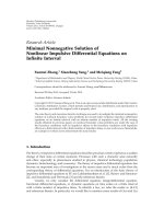
order of reference is shown in Figure 2(b). Assume that the
disk is spinning counterclockwisely and consider the follow-
ing client request sequence a, f , b, c, d, a, f , g, e, c, d, shown
in Figure 2. Note that dashed lines mean that the first ele-
ment in the request sequence (counted from left to right)
would like to fetch the first item supplied by disk, and di-
rected gr aph denotes the rotation of disk layout in a counter-
clockwise way. For this request, if we have the access sched-
ule (a, b, c, d, e, f , g), which dose not take into account the
rules, the total I/O access times for the client will be a :5,
f :5,b :3,c :2,d :6,a :5,f :5,g :1,e :5,c :6,
d : 6. The total access times is 49 and the average latency will
be 49/11
= 4.454. However, if we partition the items to be
accessed into two groups with respect to the sequential pat-
terns obtained after mining, then we will have
{a, b, f } and
{c, d, e, g}. Note that data items that appear in the same se-
quential pattern are placed in the same group. When we sort
the data items in the same group with respect to the rules
a
⇒ f and c ⇒ d, we will have the sequences (a, f , b)and
(c, d, g, e). If we organize the data items to be accessed with
respect to these sorted groups of items, we will have the ac-
cess schedule presented in Figure 2(b). In this case, the total
access times for the client for the same request pattern will be
a :1,f :1,b :1,c :1,d :1,a :3,f :1,g :4,e :1,c :4,

d : 1. The total access times is 19 and the average latency will
be 19/11
= 1.727, which is much lower than 4.454.
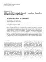
Another example that demonstrates the benefits of rule-
based prefetching is show n in Figure 3. We demonstrate three
different requests of a client as a snapshot. With the help of
the rules obtained from the history of previous requests, the
prediction can be achieved. The current request is c and there
is a r ule stating that if data item c is requested, then data item
d will be also be requested (i.e., association rule c
⇒ d). In
Figure 3(a),dataitemd is absent in the cache and the client
must spend more waiting time for item d.InFigure 3(b),
although the item d is also absent in the cache, the client
still spends one disk latency time for item d.InFigure 3(c),
the cache can supply the item d and no disk latency time is
needed.
6 EURASIP Journal on Advances in Signal Processing
Request sequence afbcdafgecd
cd
b
e
a
f
g
(a)
Request sequence afbcdafgecd
a
e
g

fd
bc
(b)
Figure 2: Effects on accessed objects organization in disk: (a) without association rules; (b) with association rules.
Cache Request sequence
b
g
acdb
···
ab
f
g
ec
d
(a)
Cache Request sequence
b
d
g
cdb
···
d
eb
f
ac
g
(b)
Cache Request sequence
b
g

dcdb
···
a
e
g
f
bc
d
(c)
Figure 3: Effects of prefetching.
These simple examples show that with some intelli-
gent grouping, reorganization of data items with predictive
prefetching, average latency for clients can be considerably
improved. In the following sections, we describe how we can
extract sequential patterns out of client requests. We also ex-
plain how we group data items with respect to sequential pat-
terns.
4. TRAVERSAL HISTORIES MINING AND
PROBLEM FORMULATION
In this section, we describe the idea and the detailed steps of
mining algorithm and give a demonstration example for this.
In order to mine sequential patterns, we assume that the con-
tinuous client requests are organized into discrete sessions.
Sessions specify user interest periods and a session consists of
a sequence of client requests for data items ordered with re-
spect to the time of reference. The client request consists of
the objects which a client browses and traverses at will in the
VEs. We denote this type of clients request as a view. A ses-
sion consists of one or more views. In correspondence with
terminologies used in data mining, a session can be consid-

ered as a sequence. The whole database is considered as a set
of sequences. Formally, let

={
l
1
, l
2
, , l
m
} be a set of m
literals, called objects (also called items)[61, 62]. The view
v is defined as snapshot of sets of objects which a user ob-
serves during the period. A view (also called itemset)isan
unordered nonempty set of objects. A sequence is an ordered
list of views. We denote a sequence s (also called transaction)
by
{v
1
, v
2
, , v
n
},wherev
j
is a view and ordered property is
obeyed. We also call v
j
an element of the sequence. An item
can occur only once in an element of a sequence, but can oc-

cur multiple times in different elements. We assume, without
loss of generality, that items in an element of a sequence are
in lexicographical order.
Asequence
a
1
a
2
···a
n
 is contained in another se-
quence
b
1
b
2
···b
m
 if there exist integers i
1
<i
2
< ··· <i
n
such that a
1
⊆ b
i
1
, a

2
⊆ b
i
2
, , a
n
⊆ b
i
n
.Forexample,
(a)(b, c)(a, d, e) is contained in (a, b)(b, c)(a, b, d, e, f ),
since (a)
⊆ (a, b), (b, c) ⊆ (b, c), and (a, d, e) ⊆ (a, b, d, e, f ).
However, the sequence
(c)(d) is not contained in (c, d)
and vice versa. The former represents objects c and d being
observed one after the other, while the latter represents ob-
jects c and d being observed together. In a set of sequences,
asequences is maximal if s is not contained in any other se-
quence. Let the database D be a set of sequences ordered by
increasing recording time. Each sequence records each user’s
traversal path in the VEs. The support for a sequence is de-
fined as the fraction of D that “contains” this sequence. A
sequential pattern p is a sequence whose support is equal to
or more than the user-defined threshold. Sequential patter
mining is the process of extracting certain sequential patterns
whose support exceeds a predefined minimal support thresh-
old.
Given a database D of client transactions, the problem of
mining sequential patterns is to find the maximal sequences

S S. Hung and D. S M. Liu 7
among all sequences that have a certain user-specified mini-
mum support. Each maximal sequence represents a sequen-
tial pattern.
Sequential rules are obtained from sequential patterns.
For a sequential pattern p
=p
1
, p
2
, , p
k
. The possible
sequential rules are

p
1

=⇒

p
2
, p
3
, , p
k

,

p

1
, p
2

=⇒

p
3
, p
4
, , p
k

,
.
.
.

p
1
, p
2
, p
3
, , p
k−1

=⇒

p

k

.
(1)
A sequential rule such as
P
n
=

p
1
, p
2
, p
n

=⇒

p
n+1
, p
n+2
, , p
k

,(2)
where 0 <n<k, has confidence c if c % of the sequences that
support
p
1

, p
2
, , p
n
 also support p
1
, p
2
, , p
k
, that is,
confidence

p
n

=
support

p
1
, p
2
, , p
k

support

p
1

, p
2
, , p
n

×
100%. (3)
For a sequential pattern p
=p
1
, p
2
, , p
k
, among the
possible rules that can be derived from p, we are interested in
the rules with the smallest possible antecedent (i.e., the first
part of the r u le). This is due to the fact that the rules used
for inferring should start as early as possible. The rest of the
rules trivially meet the confidence requirement [59].
Finally, we will define our problem in two phases. Phase
I: given a sequence database D
={s
1
, s
2
, , s
n
},wedesign
efficient mining algorithms to obtain our sequential patterns

P; Phase II: in order to reduce the disk access time, we dis-
tribute P into a set of clusters, so as to minimize intercluster
similarity and maximize intracluster similarity.
5. PATTERN-ORIENTED MINING AND
CLUSTERING ALGORITHMS
In many applications, it is not unusual that one may en-
counter a large number of sequential patterns. Similarly, our
virtual environments consist of many complex objects. These
relationships are always behind the scenes. Therefore, it is
important to explore a new efficient and scalable method.
With this motivation, we developed a sequential pattern
mining method, cal led view-based sequence pattern mining
(VSPM). Its general idea is to use frequent items to recur-
sively project sequence databases into a set of smaller pro-
jected databases and grow subsequence fragments in each
projected database. This process partitions both the data and
setoffrequentsequentialpatternstobetested,andconfines
each test being conducted to the corresponding smal ler pro-
jected database.
Before we describe our algorithm, some definitions and
conventions are presented. Since items within an element of a
sequence can be listed in any order, without loss of generality,
we assume they are listed in alphabetical order. For example,
the sequence is listed as
(a)(a, b, c, d)(a, d)(e)(c, f ) instead
of
(a)(b, c, a, d)(d, a)(e)( f , c). With such a convention, the
expression of a sequence is unique.
Definition 1 (prefix). Suppose a ll items in an element are
listed alphabetically. Given a sequence α

=α
1
α
2
···α
n
,
and a sequence β
=β
1
β
2
···β
m
,(m ≤ n)iscalledaprefix
of α if and only if (1) β
i
= α
i
for (i ≤ m − 1); (2) β
m
⊆ α
m
;
(3) all the items in (α
m
− β
m
) are alphabetically after those in
β

m
.
Definition 2 (projection). Given sequences α and β such that
β is a subsequence of α,denoteβ
 α.Asubsequenceα

of sequence α (i.e., α

 α)iscalledaprojection of α with
respect t o prefix β if and only if (1) α

has prefix β; (2) there
exists no proper supersequence α

of α

(i.e., α

 α

but
α

= α

) such that α

is a subsequence of α and also has
prefix β.
For example,

a, a,a, a(a,b), a(a,b, c),and(a)(a,
b, c)a
 areallprefixesofsequence(a)(a, b, c)(a, c, d)(d)(c, e
f )
, but the sequences a, b, a, c, a(b, c),and(a)(a, c)
are all not considered as prefixes.
5.1. View-based sequential pattern
mining algorithm
Now, we will explain our mining algorithms. The main ideas
come from both bounded-projection and pattern appending
mechanisms. The bounded-projection mechanism has one
special char acteristic, that is, it always projects the remaining
sequence recursively after a new sequential pattern is found.
They will not mine the objects across different prefix views
though. As a result, we would mine the trimmed database
recursively. The pattern appending mechanism uses the con-
cept of prefix property. When we want to find a new sequen-
tial pattern in our database, we use the sequential pattern
foundinpreviousroundasprefix,andappendanewob-
ject as the new candidate pattern for verification. If the can-
didate pattern satisfies the minimum support, we regard it
as a new sequential pattern and create a bounded projection
of it recursively. In order to explore the interesting relation-
ships among these objects, we propose two different kinds
of appending methods called intraview-appending method
and interview-appending method. The int raview-appending
method is used to append a ne w object in the same view,and
the interview-appending method is used to append a new ob-
ject in the next view. Demonstration example will be given
later. The following is the pseudocode of view sequence min-

ing algorithm (Algorithm 1).
Example 3 (VSPM). Given the traversal database S and
min
support = 3, we demonstrate the complete steps as fol-
lows:
Path1:
(1, 2)(3, 4)(5, 6);
Path2:
(1, 2)(3, 4)(5);
Path3:
(1, 2)(3)(4, 5).
Step 1 (find frequent patterns with length-1. //in the form
of “ite m: support”). First, we will have the following data:
1:3,2:3,3:3,4:3,5:3,6:1.Therefore,wehave
length-1 frequent sequential patterns:
1, 2, 3, 4,and
8 EURASIP Journal on Advances in Signal Processing
//D is the database. P is the set of frequent patterns, and is set
to empty initially.
Input: D and P.
Output: P.
Begin
(1) Find length-1 frequent sequential patterns.
(2) While (any projected subdatabase exits) do
(3) Begin
(4) Project corresponding subsequences into
sub-databases under the intraview appending and
interview appending.
(5) Mine each subdatabase corresponding to each
projected subsequence.

(6) Find all frequent sequential patterns by applying
Steps 4 and 5 on the subdatabases recursively.
(7) End; // while
(8) return P;
(9) End;//procedure
Algorithm 1: View-based sequential pattern mining (VSPM) al-
gorithm.
5. Finally, we will have 5 projection-based subdatabases
1 DB, 2 DB, 3 DB, 4 DB, and 5 DB, respectively.
Step 2. Take the projection-based subdatabase
1 DB for
example. First, since item 2 and item 1 are in same view, the
intraview appending works. After the projection, we will get
the sub-database
(1, 2) DB. And the original database is
shrunk to the following database:
P1:
(3, 4)(5, 6);P2:(3, 4)(5);P3:(3)(4, 5).
In this step, pattern
(1, 2) becomes a frequent sequent
pattern since its support satisfies the minimum support.
Next, item 3 is projected for the candidate.
Step 3 (continued from Step 2). Since item 3 and (1,2) are
in different views, the interview appending works. We will
have the projection-based subdatabase
(1, 2)(3) DB and
the shrunk database is as follows:
P1:
(4)(5, 6);P2:(4)(5);P3:(4, 5).
In this step, pattern

(1, 2)(3) becomes a frequent se-
quential pattern since its support satisfies the minimum sup-
port. Next, item 4 is projected for the candidate.
Step 4 (continued from Step 3). Since item 4 and item 3 are
in the same view, the intraview appending works. We will
have the projection-based subdatabase
(1, 2)(3, 4) DB and
the shrunk database is as follows:
P1:
(5, 6);P2:(5);P3:(5).
In this step, pattern
(1, 2)(3, 4) becomes an infrequent
sequent pattern since its support does not satisfy the mini-
mum support. The VSPM stops further mining and returns
to the previous subdatabase
(1, 2)(3) DB recursively. Next,
item 5 is projected for the candidate.
Step 5 (continued from Step 4). Since item 5 and item 3
are in different views, the interview appending works. We
will have the projection-based subdatabase
(1, 2)(3)(5) DB
and the result is as follows:
P1:
(6);P2:∅;P3:∅.
In this step, pattern
(1, 2)(3)(5) becomes an infrequent
sequent pattern since its support does not satisfy the mini-
mum support. The VSPM stops further mining and goes to
the previous subdatabase
(1, 2) DB recursively. Note that

item 6 will be discarded since item 6 is not a length-1 frequent
sequential pattern. We observe that subdatabase
(1, 2) DB
could not have any projected subdatabase through the in-
traview mining. Apparently, only item 2 and item 1 are in
the same view, other items are not. Therefore, we return to
the previous subdatabase
(1) DB recursively.
Step 6 (continued from Step 5). Since item 3 and item 1 are
in different views, the interview appending works. We will
have the projection-based subdatabase
(1)(3)) DB and the
result is as follows:
P1:
(4)(5, 6);P2:(4)(5);P3:(4, 5).
In this step, pattern
(1)(3) becomes a frequent sequen-
tial pattern since its support satisfies the minimum support.
Step 7. the remaining steps are the same as the above.
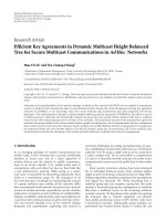
The final mining result is depicted in Figure 4.InFigure 4,
the patterns which contain item 6 are circled. They show
that the differences between projected-based mining and
nonprojected-based mining. In other words, without pro-
jecting mechanism, we have to expand eight subdatabases
for candidates (i.e., two “stop” without circled plus six “stop”
with circled). Compared to this case, with projecting mech-
anism, we only expand two subdatabases for candidates (i.e.,
“stop” without circled).
5.2. Disk organization by clustering
sequential patterns

Clustering is a good candidate for inferring object correla-
tions in storage systems. As the previous sections mentioned,
object correlations can be exploited to improve storage sys-
tem performance. First, correlations can be used to direct
prefetching. For example, if a strong correlation exists be-
tween objects a and b, these two objects can be fetched to-
gether from disks whenever one of them is a ccessed. The
disk read-ahead optimization is an example of exploiting
the simple data correlations by prefetching subsequent disk
blocks ahead of time. Several studies [46, 55–57] have shown
that u sing these correlations can significantly improve the
storage system performance. Our results in Section 6.2.2
demonstrate that prefetching based on object correlations
can improve the performance much better than that of non-
correlationlayoutinallcases.
A storage system can also organize data is disks accord-
ing to object correlations. For example, an object can be
placed next to its correlated objects so that they can be
S S. Hung and D. S M. Liu 9
Original database
Length-1 projected
subdatabase
1 DB
2 DB
3 DB 4 DB 5 DB
··· ··· ··· ···

(1, 2) DB (1)(3) DB (1, 4) DB (1)(5) DB
Interview
Intraview

Interview
Interview Interview Interview Intraview Interview
Interview
(1, 2)(3) DB Nonexist
(1)(3, 4) DB
Stop
(1)(3(5) DB
(1)(3)(6) DB
Stop
(1)(4)(5) DB
(1)(4)(6) DB
Stop
(1)(5, 6) DB
Stop
Nonexist
Intraview Interview
Intraview
Intraview
(1, 2)(3, 4) DB (1, 2)(3)(5) DB (1)(4)(5, 6) DB
Stop
Stop
Stop
Intraview Interview
(1)(3)(5, 6) DB
(1, 2)(3)(5, 6) DB
Nonexist
Stop
Figure 4: Demonstration of our VSPM for generating projected-based subdatabases and sequential patterns.
fetched together using just one disk access. This optimization
can reduce the number of disk seeks and rotations, which

dominate the average disk access latency. With correlation-
directed disk layouts, the system only needs to pay a cost of
one-time seek and a rotational delay to get multiple objects
that are likely to be accessed soon. Previous studies [55, 56]
have shown promising results in allocating correlated file
blocks on the same track to avoid track-switching costs.
The main idea of our clustering approach is to define a
new notion of cluster centroid, which represents the com-
mon properties of cluster elements. Similarity inside a cluster
is hence measured by using the cluster representative. The
cluster representative becomes a natural tool for finding an
explanation of the cluster population. Our definition of clus-
ter centroid is based on a data representation model which
simplifies the ones used in pattern clustering. In fact, we use
compact representation of Boolean vector v that states only
presence or absence of items, while traditional pattern clus-
tering methods require to store the frequencies of items. In
this paper, we show that using our concept of cluster cen-
troid associated with Jaccard distance [53], we obtain results
that have a quality comparable with other approaches used in
this kind of task, but we have better performances in terms of
ex ecution time. Moreover, cluster representatives provide an
immediate explanation of cluster features.
5.3. Distance measure
In the simplified hypothesis that frequent patterns do not
contain frequencies, but behave simple as Boolean vectors
(like value 1 corresponds to the presence and value 0 corre-
sponds to the absence), a more intuitive but e quivalent way
of defining the Jaccard distance function can be provided. This
measure captures our idea of similarit y between items that is

directly proportional to the number of common values, and
inversely proportional to the number of different values for
the same item.
Definition 4 (intradistance measure (cooccurrence)). Let P
1
and P
2
be two sequential patterns. D(P
1
, P
2
)canberepre-
sented as the normalized difference between the cardinality
of their union and the cardinality of their intersection:
D

P
1
, P
2

=
1 −


P
1
∩ P
2





P
1
∪ P
2


. (4)
Example 5 (intradistance measure). Let P
1
and P
2
be two se-
quential patterns: P
1
=(a, b, c), (b, c, d), (e, f ) and P
2
=

(a, b, c, d), (e, f , g). The distance between P
1
and P
2
is
D

P
1

, P
2

=
1 −


P
1
∩ P
2




P
1
∪ P
2


=
1 −


{
a, b, c, e, f }





{
a, b, c, d, e, f , g}


=
1 −
5
7
=
2
7
.
(5)
5.4. Cluster representative and pattern
clustering algorithm
Intuitively, a cluster representative for virtual environment
data should model the content of a cluster, in terms of the ob-
jects that are most likely to appear in a pattern belonging to
the cluster. A problem with the traditional distance measures
is that the computation of a cluster representative is compu-
tationally expensive. As a consequence, most approaches [38]
approximate the cluster representative with the Euclidean
representative. However, those approaches may suffer the fol-
lowing drawbacks.
(i) Huge cluster representatives cause poor performances,
mainly because as soon as the clusters are populated,
the cluster representatives are likely to become ex-
tremely huge.
(ii) For different kinds of patterns, it seems to be difficult

to find the proper cluster representatives.
In order to overcome such problems, we can compute an
approximation that resembles the cluster representatives as-
sociated to Euclidean and mismatch-count distances. Union
and intersection seem good candidates to start with. Since
our clustering operations are based on set operations, we ig-
nore the order of frequent patterns.
To avoid these undesired situations, we supply three ta-
bles. The first table is FreqTable. It records the frequency of
10 EURASIP Journal on Advances in Signal Processing
// P is the set of frequent patterns. T is the set of clusters, and
is set to empt y initially.
Input: P and T.
Output: T.
Begin
(1) FreqTable
= { ft
ij
| the frequency of pattern
i
and
pattern
j
coexisting in the database D};
(2) DistTable
= {dt
ij
| the distance between
pattern
i

and pattern
j
in the database D};
(3) C
1
={C
i
| at the beginning each pattern to
be a single cluster}
(4) // Set up the extra-similarity table for evaluation
(5) M
1
= Intrasimilar (C
1
, ∅);
(6) k
= 1;
(7) while
|C
k
|n do Beg in
(8)
C
k+1
= PatternCluster (C
k
, M
k
, FreqTable, DistTable);
(9) M

k+1
= Intrasimilar (C
k+1
, M
k
);
(10) k
= k +1;
(11) End;
(12) return C
k
;
(13) End;
Algorithm 2: Pattern clustering algorithm.
any two patterns coexisting in the database D. The second ta-
ble is DistTable. It records the distance between any two pat-
terns. The last table is Cluster. It records how many clusters
are generated. Algorithm 2 is our clustering algorithm.
Consider a database of learner transactions shown in
Tab le 3. For each transaction, we keep the transaction’s time,
objects accessed in the VR system, and a unique learner
identifier. Tabl e 4 shows an alternative representation of the
database, where an ordered set of purchased items is given
for each learner.
Let us assume that the system wants to cluster these users
according to the similar frequent objects into three clusters.
Tab le 5 shows frequent sequential patterns discovered in the
database shown in Table 4 (with minimum support >25%).
The intermediate results of clustering starting at the third
iteration to the eighth iteration are presented in Tables 8

to 13, respectively. The following relations between patterns
hold: P
2
⊂ P
1
, P
3
⊂ P
1
, P
4
⊂ P
1
, P
5
⊂ P
1
, P
6
⊂ P
1
, P
7
⊂ P
1
,
P
5
⊂ P
2

, P
6
⊂ P
2
, P
5
⊂ P
3
, P
7
⊂ P
3
, P
6
⊂ P
4
, P
7
⊂ P
4
,
P
9
⊂ P
8
,andP
10
⊂ P
8
. This leads to removing P

8
from
the description of cluster C
ahij
,andP
2
, P
3
,andP
4
from the
description of cluster C
bcde f g
because each of them includes
some other patterns from the same description, for example
P
9
⊂ P
8
, and they are both in the description of cluster C
ahij
.
After completion of the description pruning step, we get the
final result of clustering shown in Table 14.
6. SYSTEM ARCHITECTURE AND
PERFORMANCE EVALUATION
We implemented the data mining algorithms and prefetching
mechanisms to show the effectiveness of the proposed meth-
ods. A traversal path database recorded each user’s traversal
path and was used for mining interesting patterns. The sim-

Table 3: Database sorted by user ID and tr ansaction time.
User ID Transaction time Objects accessed
1 17:30 PM Sep 9. 2005 10 60
1 17:37 PM Sep 9. 2005 20 30
1 17:45 PM Sep 9. 2005 40
1 17:55 PM Sep 9. 2005 50 55
2 16:30 PM Sep 10. 2005 40
2 16:37 PM Sep 10. 2005 50
2 17:00 PM Sep 10. 2005 10
2 17:30 PM Sep 10. 2005 20 30 70
3 12:33 PM Sep 11. 2005 40
3 12:38 PM Sep 11. 2005 50
3 13:00 PM Sep 11. 2005 10
3 13:36 PM Sep 11. 2005 80
3 13:45 PM Sep 11. 2005 20 30
4 16:35 PM Sep 12. 2005 10
4 17:30 PM Sep 12. 2005 20 55
5 17:34 PM Sep 13. 2005 80
6 15:23 PM Sep 12. 2005 10
6 15:30 PM Sep 12. 2005 30 90
7 17:30 PM Sep 10. 2005 20 30
8 16:13 PM Sep 13. 2005 60
8 16:32 PM Sep 13. 2005 100
9 16:36 PM Sep 13. 2005 100
10 16:45 PM Sep 14. 2005 90 100
Table 4: User-sequence representation of the database.
User ID Traversal sequence
1

(10 60) (20 30) (40) (50 55)


2

(40) (50) (10) (20 30 70)

3

(40) (50) (10) (80) (20 30)

4

(10) (20 55)

5

(80)

6

(10) (30 90)

7

(20) (30)

8

(60) (100)

9


(100)

10

(90 100)

ulation model we used and the experimental results are pro-
vided in Sections 6.1 and 6.2,respectively.
6.1. Test data and simulation model
We use the virtual power plant model from http://www
.cs.unc.edu/
∼walk/ created by Walkthrough Labora tory of
Department of Computer Science of University of North
Carolina at Chapel Hill. The power plant model is a complete
model of an actual coal fired power plant. The model consists
of 12, 748, 510 triangles. Its size is 334 megabytes. Our traver-
sal database keeps track of the traversal of the power plant
by many anonymous random users. For each user, the data
records list all the areas of the power plant that user visited in
S S. Hung and D. S M. Liu 11
Table 5: Pattern set used for clustering.
Patterens with support > 25%
P
1

(10) (20 30)

P
2


(10) (20)

P
3

(10) (30)

P
4

(20 30)

P
5

(10)

P
6

(20)

P
7

(30)

P
8


(40) (50)

P
9

(40)

P
10

(50)

P
11

(100)

Table 6: Pattern-oriented representation of the database.
Cluster Description Sequences
C
a
P
1
1, 2, 3
C
b
P
2
1, 2, 3, 4

C
c
P
3
1, 2, 3, 6
C
d
P
4
1, 2, 3, 7
C
e
P
5
1, 2, 3, 4, 6
C
f
P
6
1, 2, 3, 4, 7
C
g
P
7
1, 2, 3, 6, 7
C
h
P
8
1, 2, 3

C
i
P
9
1, 2, 3
C
j
P
10
1, 2, 3
C
k
P
11
8, 9, 10
Table 7: Initial similarity matrix.
C
a
C
b
C
c
C
d
C
e
C
f
C
g

C
h
C
i
C
j
C
k
C
a
x 0.75 0.75 0.75 0.6 0.6 0.6 1 1 1 0
C
b
0.75 x 0.6 0.6 0.8 0.8 0.5 0.75 0.75 0.75 0
C
c
0.75 0.6 x 0.6 0.8 0.5 0.8 0.75 0.75 0.75 0
C
d
0.75 0.6 0.6 x 0.5 0.8 0.8 0.75 0.75 0.75 0
C
e
0.6 0.8 0.8 0.5 x 0.66 0.66 0.6 0.6 0.6 0
C
f
0.6 0.8 0.5 0.8 0.66 x 0.66 0.6 0.6 0.6 0
C
g
0.6 0.5 0.9 0.8 0.66 0.6 x 0.6 0.6 0.6 0
C

h
1 0.75 0.75 0.75 0.6 0.6 0.6 x 1 1 0
C
i
1 0.75 0.75 0.75 0.6 0.6 0.6 1 x 1 0
C
j
1 0.75 0.75 0.75 0.6 0.6 0.6 1 1 x 0
C
k
0000000000x
a one-week t imeframe. Each path consists of 30 ∼ 40 views.
Each view consists of 20 ∼ 30 objects on average. The num-
ber of objects is 11, 949, where each object is a meaningful
combination of triangles of power plant and it is considered
as a data item. On the other side, the whole system consists
of four parts: (1) log-data manager; (2) mining unit; (3) clus-
tering unit; (4) storage manager.
The log-data manager performs the interaction between
the user and power plant, and records the states which the
user visited. The mining unit performs the task of extract-
ing sequential patterns and rules from the traversal database.
Rules set with different minimum support requirements can
be constructed by the mining unit. The resulting sequential
patterns are written to a file in a specific format to be read
later by the clustering unit and storage manager. The cluster-
ing unit performs clustering of data items using our cluster-
ing algorithm based on the sequential patterns. After cluster-
ing, the clusters are placed into the disk block for prefetching.
The architecture of our system is depicted in Figure 5.In

this architecture, we use the traversal database to simulate the
access history. The sequence of traversal paths that are orga-
nized into views is fed into the data mining programs to be
used for extracting sequential patterns. The resulting pattern
set is fed into the clustering unit, which is then used for disk
organization and prefecthing.
As we present i n Figure 5, we summarize the main steps
as follows. First, each user enters into the VEs using the
user interface. The interface will send one request handle
to acquire the service from the system. The system not only
records the views along the traversal path for each user, but
also processes these views into appropriate data format for
later mining. Second, the mining unit performs the mining
tasks according to our mining algorithms. After the comple-
tion of mining phase, the clustering unit will take over the
remaining work—clustering the patterns. Finally, when the
clustering phase ends, the final clusters will enable predicting
the next view request of users.
6.2. Experimental results and performance study
In this section, the effectiveness of the proposed cluster-
ing algorithm is investigated. All algorithms were imple-
mented in Java. The experiments were run on a PC with
an AMD Athlon 1800+ and 512 megabytes main memory,
running Microsoft Windows 2000 server. Our main perfor-
mance met ric is the average latency. We also measured the
client cache hit ratio. A decrease in the average latency is an
indication of how useful the proposed methods are. The av-
erage latency can decrease as a result of both increase cache
hit ratio via prefetching methods and better data organiza-
tion in the disk. An increase in the cache hit ratio will also

decrease the number of requests sent to server, and thus lead
to both saving of the scare memory resource of the server and
reduction in the server load.
We have two major tasks—mining algorithm and clus-
tering algorithm. We report our experimental results on the
performance of mining and clustering, respectively.
6.2.1. Experimental results on mining unit
In this section, we repor t our experimental results on the
VSPM algorithm. Since GSP and SPADE are the two most
important sequential pattern mining algorithms, we con-
duct an extensive perfor m ance study to compare VSPM with
them. To evaluate the effectiveness and efficiency of the
VSPM algorithm, we performed an extensive performance
study of GSP, SPADE, FreeSpan,andPrefixSpan,onbothreal
and synthetic datasets, with various kinds of sizes and data
12 EURASIP Journal on Advances in Signal Processing
Table 8: Similarity matrix and database after 3rd iteration.
C
ahij
C
b
C
c
C
d
C
e
C
f
C

g
C
k
C
ahij
x 0.75 0.75 0.75 0.6 0.6 0.6 0
C
b
0.75 x 0.6 0.6 0.8 0.8 0.5 0
C
c
0.75 0.6 x 0.6 0.8 0.5 0.8 0
C
d
0.75 0.6 0.6 x 0.5 0.8 0.8 0
C
e
0.6 0.8 0.8 0.5 x 0.66 0.66 0
C
f
0.6 0.8 0.5 0.8 0.66 x 0.66 0
C
g
0.6 0.5 0.8 0.8 0.66 0.66 x 0
C
k
0000000x
Cluster Description Sequences
C
ahij

P
1
, P
8
, P
9
, P
10
1, 2, 3
C
b
P
2
1, 2, 3, 4
C
c
P
3
1, 2, 3, 6
C
d
P
4
1, 2, 3, 7
C
e
P
5
1, 2, 3, 4, 6
C

f
P
6
1, 2, 3, 4, 7
C
g
P
7
1, 2, 3, 6, 7
C
k
P
11
8, 9, 10
Table 9: Similarity matrix and database after 4th iteration.
C
ahij
C
be
C
c
C
d
C
f
C
g
C
k
C

ahij
x 0.6 0.75 0.75 0.6 0.6 0
C
be
0.6 x 0.8 0.5 0.66 0.66 0
C
c
0.75 0.8 x 0.6 0.5 0.8 0
C
d
0.75 0.5 0.6 x 0.8 0.8 0
C
f
0.6 0.66 0.5 0.8 x 0.66 0
C
g
0.6 0.66 0.8 0.8 0.66 x 0
C
k
000000x
Cluster Description Sequences
C
ahij
P
1
, P
8
, P
9
, P

10
1, 2, 3
C
be
P
2
, P
5
1, 2, 3, 4, 6
C
c
P
3
1, 2, 3, 6
C
d
P
4
1, 2, 3, 7
C
f
P
6
1, 2, 3, 4, 7
C
g
P
7
1, 2, 3, 6, 7
C

k
P
11
8, 9, 10
Table 10: Similarity matrix and database after 5th iteration.
C
ahij
C
bce
C
d
C
f
C
g
C
k
C
ahij
x 0.6 0.75 0.6 0.6 0
C
bce
0.6 x 0.5 0.66 0.66 0
C
d
0.75 0.5 x 0.8 0.8 0
C
f
0.6 0.66 0.8 x 0.66 0
C

g
0.6 0.66 0.8 0.66 x 0
C
k
00000x
Cluster Description Sequences
C
ahij
P
1
, P
8
, P
9
, P
10
1, 2, 3
C
bce
P
2
, P
3
, P
5
1, 2, 3, 4, 6
C
d
P
4

1, 2, 3, 7
C
f
P
6
1, 2, 3, 4, 7
C
g
P
7
1, 2, 3, 6, 7
C
k
P
11
8, 9, 10
Table 11: Similarity matrix and database after 6th iteration.
C
ahij
C
bce
C
df
C
g
C
k
C
ahij
x 0.6 0.6 0.6 0

C
bce
0.6 x 0.66 0.66 0
C
df
0.6 0.66 x 0.66 0
C
g
0.6 0.66 0.66 x 0
C
k
0000x
Cluster Description Sequences
C
ahij
P
1
, P
8
, P
9
, P
10
1, 2, 3
C
bce
P
2
, P
3

, P
5
1, 2, 3, 4, 6
C
df
P
4
, P
6
1, 2, 3, 4, 7
C
g
P
7
1, 2, 3, 6, 7
C
k
P
11
8, 9, 10
Table 12: Similarity matrix and database after 7th iteration.
C
ahij
C
bcde f
C
g
C
k
C

ahij
x0.50.60
C
bcde f
0.5 x 0.83 0
C
g
0.6 0.83 x 0
C
k
00 0x
Cluster Description Sequences
C
ahij
P
1
, P
8
, P
9
, P
10
1, 2, 3
C
bcde f
P
2
, P
3
,P

4
, P
5
, P
6
1, 2, 3, 4, 6, 7
C
g
P
7
1, 2, 3, 6, 7
C
k
P
11
8, 9, 10
S S. Hung and D. S M. Liu 13
Table 13: Similarity and database after 8th iteration.
C
ahij
C
bcde f
C
g
C
k
C
ahij
x0.50.60
C

bcde f
0.5 x 0.83 0
C
g
0.6 0.83 x 0
C
k
00 0x
Cluster Description Sequences
C
ahij
P
1
, P
8
, P
9
, P
10
1, 2, 3
C
bcde f g
P
2
, P
3
,P
4
, P
6

, P
5
, P
7
1, 2, 3, 4, 6, 7
C
k
P
11
8, 9, 10
Table 14: Discovered clusters.
Cluster Description Sequences
C
ahij
P
1
=

(10) (20 30)

, P
9
=

(40)

, P
10
=


(50)

1, 2, 3
C
bcde f g
P
5
=

(10)

, P
6
=

(20)

P
7
=

(30)

1, 2, 3, 4, 6, 7
C
k
P
11
=


(100)

8, 9, 10
distributions. Four algorithms, GSP, SPADE, FreeSpan,and
PrefixSpan were implemented in Java. Detailed algorithm im-
plementation is described as follows: (1) GSP, the GSP algo-
rithm is implemented according to the description in [59];
(2) SPADE, the SPADE algorithm is implemented according
to the description in [44]; (3) FreeSpan, the FreeSpan algo-
rithm is implemented according to the description in [16];
(4) PrefixSpan, the PrefixSpan algorithm with level-by-level
projection is implemented according to the description in
[15].
For the datasets used in our performance study, we use
two kinds of datasets: one real dataset andagroupofsyn-
thetic datasets. The synthetic datasets used in our exper-
iments were generated using the standard procedure de-
scribedin[42]. The same data generator has been used in
most studies on sequential pattern mining, such as [15, 16,
59]. For real dataset, we have obtained our traversal database.
For synthetic datasets, we have also used a large set of
synthetic sequence data generated by the IBM data genera-
tor [42] designed for testing sequential patterns mining algo-
rithm. Since the format of such datasets has its specific mean-
ings, we explain the convention for the datasets as follows.
For example, C200T2.5S10I1.25 means that the dataset con-
tains 200 k sequences (denoted as C200) and the number of
items is 10 000. The average number of items in a transaction
is 2.5 (denoted as T2.5), and the average number of transac-
tions in a sequence is 10 (denoted as S10). On average, each

transaction is composed of 1.25 items (denoted as I1.25).
Synthetic dataset experiments
The first test is performed on the dataset C200T2.5S10I1.25.
It contains 200 k transactions and the number of items is
10 000. Figure 6 shows the processing time of the five algo-
rithms at different support thresholds. The processing times
are sort ed in time ascending order as “PrefixSpan < VSPM
< SPADE < FreeSpan < GSP.” When the support threshold
is set to 0.4%, the running time of PrefixSpan is 12.374 sec-
onds. Under the same condition, the running time of our al-
gorithm (VSPM) is 19.736 seconds. Compared to other algo-
rithms, the running times of SPADE, FreeSpan,andGSP are
26.478, 35.949, 91.595 seconds, respectively. When the sup-
port threshold drops to 0.3%, the running time of PrefixSpan
is 19.948 seconds. Similarly, our running time is 27.857 sec-
onds. Compared to other algorithms, the running times of
SPADE, FreeSpan,andGSP are 37.475, 89.459, 188.895 sec-
onds, respectively.
The second test is performed on the data set C10T8S8I8.
It contains 10 K transactions and the number of items is still
10 000. Figure 7 shows the processing time of the five algo-
rithms at different support thresholds. The processing times
are sorted in time ascending order as “PrefixSpan < VSPM <
SPADE < FreeSpan < GSP.” When the support threshold is set
to 1%, the ru nning time of PrefixSpan is 8.785 seconds. Un-
der the same condition, the running time of our algorithm
(VSPM) is 11.783 seconds. Compared to other algorithms,
the running times of SPADE, FreeSpan,andGSP are 12.785,
79.378, 845.658 seconds, respectively. As Figure 7 shows, the
support threshold is 1%, the running time of GSP is empty.

Since the difference between any other algorithms is so sharp,
we decide that value not to be plotted in Figure 7. Similarly,
when the support threshold drops to 0.5%, the running time
of PrefixSpan is 49.369 seconds. Under the same condition,
the running time of our algorithm (VSPM) is 89.764 seconds.
Compared to other algorithms, the r u nning times of SPADE,
FreeSpan,andGSP are 109.234, 120.874, 6,685.213 seconds,
respectively. Compared with the second dataset, the first set is
larger than the second dataset since it contains more transac-
tions. However, it is sparser than the second data set since the
average number of items in a transaction is 2.5 (i.e., 2.5 < 8)
and the average number of transactions in a sequence is 10
(i.e., 10 > 8). In other words, the second data set is much
denser than the first dataset. This results in one fact that the
running time of the second dataset is more than that of the
first dataset.
Scale-up experiments
In order to verify the scalability of VSPM, we set up the fol-
lowing experimental environments. First, all five algorithms
run the test dataset T2.5S10I1.25, with the database size
growing from 200 K to 900 K transactions, and with different
14 EURASIP Journal on Advances in Signal Processing
Clustering unit Mining unit
Back end
Storage manager Low-data manager
Path
recorder
Request
handler
Path

recorder
Request
handler
Path
recorder
Request
handler
···
Front end
User
interface
User
interface
User
interface
··· Client
Figure 5: System architecture diagram.
0
10
20
30
40
50
Running time (s)
10.90.80.70.60.5
Support threshold (%)
PrefixSpan
SPADE
VSPM
FreeSpan

GSP
Figure 6: Performance of the five algorithms on dataset C200T2.5
S10I1.25.
0
20
40
60
80
100
120
140
Running time (s)
32.521.510.5
Support threshold (%)
PrefixSpan
SPADE
VSPM
FreeSpan
GSP
Figure 7: Perfor mance of the five algorithms on dataset C10T8S8I8.
support threshold settings. Since the algorithm SPADE runs
more than 1200 seconds at 900 K transactions, shown in
0
200
400
600
800
1000
1200
Running time (s)

200 300 400 500 600 700 800 900
Size of database (K transactions)
Prefix
SPADE
VSPM
FreeSpan
GSP
Figure 8: Scalability measure of the five algorithms on dataset
T2.5S10 I1.25 with support threshold
= 0.25%.
Figure 8, we cannot include this data into the figure. How-
ever, the running time of SPADE is shown in Figure 9.It
obeys the property that as the support threshold decreases,
the more candidates are genera ted and tested. As a result, the
system performance becomes worse. Moreover, the perfor-
mance of VSPM was very stable, even when support thresh-
old was very low for large databases.
Virtual environment traces
The performance of our t raversal database is reported as fol-
lows. First, we follow the procedure described in [59]toset
up dataset par ameters. Meanings of all parameters are listed
in Tab le 15. Figures 10 and 11 show the performance com-
parison among the five algorithms for our virtual environ-
ment dataset. From Figures 10 and 11, we can see that VSPM
is as efficient as PrefixSpan does, but it is much more efficient
than SPADE, FreeSpan,andGSP.
S S. Hung and D. S M. Liu 15
Table 15: Parameters for our traversal dataset.
Symbol Meaning
|D| Number of data sequences (i.e., size of database)

|C| Average number of transactions per data sequence
|T| Average number of item per transaction
|S| Average length of maximal possible frequent sequences
|I| Average size of itemsets in maximal possible frequent sequences
|N
s
| Number of maximal potentially frequent sequences
|N
I
| Number of maximal potentially frequent itemsets
|N| Number of items
0
20
40
60
80
100
120
140
Running time (s)
200 300 400 500 600 700 800 900
Size of database (K transactions)
Prefix
SPADE
VSPM
FreeSpan
GSP
Figure 9: Scalability measure of the five algorithms on dataset
T2.5S10 I1.25 with support threshold
= 0.5%.

0
20
40
60
80
100
120
140
Running time (s)
32.521.510.5
Support threshold (%)
PrefixSpan
SPADE
VSPM
FreeSpan
GSP
Figure 10: Execution time with respect to various support thresh-
olds using our real dataset-1 (daraset D1000-C40-T10-S3-T5).
6.2.2. Experimental results on clustering unit
For quality measure of clustering result, we adopted the clus-
ter cohesion and the interclustering similarity. All are defined
as follows.
0
20
40
60
80
100
120
Running time (s)

32.521.510.5
Support threshold (%)
PrefixSpan
SPADE
VSPM
FreeSpan
GSP
Figure 11: Execution time with respect to various support thresh-
olds using our real dataset-2 (dataset D750-C30-T10-S2.5-T5).
Definition 6 (large item). Given a pattern
i
and a user-defined
threshold θ, if it satisfies the criterion
0 < minimum support threshold <θ
≤ support(pattern
i
)
≤ 1, the pattern
i
is called as a large item.
Definition 7 (cluster cohesion (Cluster-Coh (C
i
))). It is the
ratio of the large items to the whole items T(C
i
) in the cluster
C
i
. This is calculated using the following formula, and if it is
near 1, it is a good quality cluster; otherwise, it is not:

Cluster-Coh

C
i

=
C
i
(L)
T

C
i

,(6)
where C
i
(L) is the number of large items in cluster C
i
,and
T(C
i
) is the number of all items in cluster C
i
.
Definition 8 (inter-cluster similarity (inter-sim (C
i
, C
j
))). It

is based on the large items is the rate of the common large
items of the cluster C
i
and C
j
. The intercluster similarity is
calculated by the following formula, and if it is near 0, it is
the good clustering; otherwise it is not:
Sim

C
i
, C
j

=
LarCom

C
i
∩ C
j

C
i
(L)+C
j
(L)
×



LarCom

C
i
∩ C
j





LarCom

C
i
+ C
j



,
(7)
where LarCom (C
i
∩ C
j
) is the number of common large
items in the clusters C
i

and C
j
, |LarCom(C
i
∩ C
j
)| is the
16 EURASIP Journal on Advances in Signal Processing
0
5
10
15
20
25
30
Total files/total views
2000 4000 6000 8000 10000 12000
View radius
Clustering
Without clustering
Figure 12: Comparison of different algorithms on the number of
files retrieved under the same view.
0
1000
2000
3000
4000
5000
6000
Response time (ms)

2000 4000 6000 8000 10000 12000
View radius
Clustering
Without clustering
Figure 13: Comparison of different algorithms on system response
time under the same view radius.
total occurrence number of the common large items, and
|LarCom(C
i
∩C
j
)| is the total occurrence number of the large
items in the clusters C
i
and C
j
.
Definition 9 (view radius). The view radius is defined as the
radius of the visible circle in the virtual environments. As the
radius increases, more objects are observed. In other words,
it controls how many objects are visible at the same time in
one view.
Meanwhile, we select the different views radius for com-
parison. Figures 12 and 13 show the results. Algorithm with
clustering outperforms other algorithms without clustering.
The clustering mechanism can accurately support prefetch-
ing objects for future usage. Not only is the access time cut
down, but also the I/O efficiency is improved.
Observing both Figures 14 and 15, we can easily realize,
there exist relations between the number of clusters and in-

tercluster similarity, and also between the number of clusters
and cluster cohesion. The less the number of clusters is, the
smaller intercluster similarity we can get. On the contrary, if
the less the number of clusters is, the larger cluster cohesion
we can get. In summary, we can determinate that our cluster-
ing algorithm is overall better at cluster cohesion and inter-
cluster similarity. This means that our clustering algorithm
0
0.2
0.4
0.6
0.8
1
Cluster cohesion
0.511.522.53
Support threshold (%)
Without clustering
Clustering
Figure 14: Comparison of different support thresholds on cluster
cohesion under the same view radius and database.
0
0.02
0.04
0.06
0.08
0.1
0.12
0.14
Intercluster similarity (&)
32.52 1.510.5

Support threshold (%)
With intercluster similarity
Without intercluster similarity
Figure 15: Comparison of different support thresholds on inter-
cluster similarity under the same view radius and database.
groups similar patterns together and improves the efficiency
of storage systems.
7. CONCLUSIONS AND FUTURE WORK
This paper proposes a VSPM, a novel approach that uses data
mining techniques to systematically mine traversal paths in a
virtual environment to infer object correlation. More specif-
ically, we have designed a frequent projection-based sequen-
tial pattern mining algorithm to find correlations among ob-
jects. Using synthetic datasets and actual virtual environ-
ments traces, our experiments show that VSPM is an ef-
ficient algorithm. We have also scaled our experiments on
VSPM for testing its scalability. Besides, we have evaluated
correlation-directed prefetching and data layout. Our exper-
imental results with virtual environments traces have shown
that correlation-directed prefetching and data layout can im-
prove I/O average response time by 35.6% to 1.249 seconds
compared to no prefetching, and 33.3% to 2.625 seconds
compared to the number of retrieved files. Finally, we have
also designed two criteria to verify the validity of clustering
method.
Our study still has limitations. First, even though this
paper focuses on how to obtain object correlations, our
S S. Hung and D. S M. Liu 17
evaluation of the object correlation-directed prefetching and
disk layout was not designed for the extra long frequent se-

quential patterns. Since the problem of long sequential pat-
terns should be customized, we are in the process of imple-
menting another long-based correlation-directed prefetch-
ing mechanism. Second, the sequential order is not main-
tained in clustering units. As this problem is concerned, we
are in the processing of designing several clustering criteria
and verify ing their validity. Finally, the disk layout should
consider not only the temporal locality, but also the spatial
locality (shown in the traversal database). This direction will
enhance the system performance.
REFERENCES
[1] S. Christodoulakis, P. Triantafillou, and F. Zioga, “Principles of
optimally placing data in tertiary storage libraries,” in Proceed-
ings of the 23rd International Conference on Very Large Data
Bases (VLDB ’97), pp. 236–245, Athens, Greece, August 1997.
[2] S. More, S. Muthukrishnan, and E. A. M. Shriver, “Effi-
ciently sequencing tape-resident jobs,” in Proceedings of the
18th ACM SIGACT-SIGMOD-SIGART Symposium on Princi-
ples of Database Systems (PODS ’99), pp. 33–43, Philadelphia,
Pa, USA, May-June 1999.
[3] S. Sarawagi, “Database systems for efficient access to te rtiary
memory,” in Proceedings of the 14th IEEE Symposium on Mass
Storage Systems (MSS ’95), pp. 120–126, Monterey, Calif, USA,
September 1995.
[4] J. Yu and D. J. Dewitt, “Processing satellite images on tertiary
storage:astudyoftheimpactoftilesizeonperformance,”in
Proceedings of the 5th NASA Goddard Conference on Mass Stor-
age Systems and Technologies, pp. 460–476, College Park, Md,
USA, September 1996.
[5] E. Thereska, M. Abd-El-Malek, J. J. Wylie, D. Narayanan, and

G. R. Ganger, “Informed data distribution selection in a self-
predicting storage system,” in Proceedings of the 3rd IEEE Inter-
national Conference on Autonomic Computing (ICAC ’06),pp.
187–198, Dublin, Ireland, June 2006.
[6] A. Amer, D. D. E. Long, J F. Paris, and R. C. Burns, “File ac-
cess prediction with adjustable accuracy,” in Proceedings of 21st
IEEE International Performance, Computing, and Communi-
cations Conference (IPCCC ’02), pp. 131–140, Phoenix, Ariz,
USA, April 2002.
[7] J. Yang, M. O. Ward, E. A. Rundensteiner, and S. Huang, “Vi-
sual hierarchical dimension reduction for exploration of high
dimensional datasets,” in Proceedings of Symposium on Visual-
ization (VisSym ’03), pp. 19–28, Grenoble, France, May 2003.
[8] P. Cignoni, C. Montani, C. Rocchini, and R. Scopigno, “Exter-
nal memory management and simplification of huge meshes,”
IEEE Transactions on Visualization and Computer Graphics,
vol. 9, no. 4, pp. 525–537, 2003.
[9] H. Hoppe, “Progressive meshes,” in Proceedings of the 23rd An-
nual Conference on Computer Graphics (SIGGRAPH ’96),pp.
99–108, New Orleans, La, USA, August 1996.
[10] S E. Yoon and D. Manocha, “Cache-efficient layouts of
bounding volume hier archies,” Computer Graphics Forum,
vol. 25, no. 3, pp. 507–516, 2006.
[11] S E. Yoon, P. Lindstrom, V. Pascucci, and D. Manocha,
“Cache-oblivious mesh layouts,” ACM Transactions on Graph-
ics, vol. 24, no. 3, pp. 886–893, 2005.
[12] S E. Yoon and P. Lindstrom, “Mesh layouts for block-based
caches,” IEEE Transactions on Visualization and Computer
Graphics, vol. 12, no. 5, pp. 1213–1220, 2006.
[13] S. Chakrabarti, Mining the Web: Discovering Knowledge from

Hypertext Data, Morgan Kaufmann, San Francisco, Calif,
USA, 2003.
[14] M S. Chen, J. S. Park, and P. S. Yu, “Efficient data mining for
path traversal patterns,” IEEE Transactions on Knowledge and
Data Engineering, vol. 10, no. 2, pp. 209–221, 1998.
[15] J. Pei, J. Han, B. Mortazavi-Asl, et al., “PrefixSpan: min-
ing sequential patterns efficiently by prefix-projected pattern
growth,” in Proceedings of the 17th International Conference on
Data Engineering (ICDE ’01), pp. 215–224, Heidelberg, Ger-
many, April 2001.
[16] J. Han, J. Pei, B. Mortazavi-Asl, Q. Chen, U. Dayal, and M.
Hsu, “FreeSpan: frequent pattern-projected sequential pattern
mining,” in Proceedings of the 6th ACM SIGKDD International
Conference on Knowledge Discovery and Data Mining (KDD
’00), pp. 355–359, Boston, Mass, USA, August 2000.
[17] R. Kohavi, C. E. Brodley, B. Frasca, L. Mason, and Z. Zheng,
“KDD-Cup 2000 organizers’ report: peeling the onion,”
SIGKDD Explorations, vol. 2, no. 2, pp. 86–98, 2000.
[18] S. Sarawagi and M. Stonebraker, “Efficient organization of
large multidimensional arrays,” in Proceedings of the 10th In-
ternat ional Conference Data Engineering (ICDE ’94), pp. 328–
336, Houston, Tex, USA, February 1994.
[19] S. More and A. Choudhary, “Tertiary storage organization
for large multidimensional datasets,” in Proceedings of the 8th
NASA Goddard Space Flight Center Conference on Mass Stor-
age Systems and Technologies in Cooperation with the 17th IEEE
Symposium on Mass Storage Systems, pp. 203–210, College
Park, Md, USA, March 2000.
[20] P. J. Rhodes and S. Ramakrishnan, “Iteration aware prefetch-
ing for remote data access,” in Proceedings of the 1st Interna-

tional Conference on e-Science and Grid Computing, pp. 279–
286, Melbourne, Australia, December 2005.
[21] W. T. Correa, J. T. Klosowski, and C. T. Silva, “Visibility-based
prefetching for interactive out-of-core rendering,” in Proceed-
ings of the IEEE Symposium on Parallel and Large-Data Visual-
ization and Graphics (PVG ’03), pp. 1–8, Seattle, Wash, USA,
October 2003.
[22] P. J. Rhodes, X. Tang, R. D. Bergeron, and T. M. Sparr, “Out-
of-core visualization using iterator-aware multidimensional
prefetching,” in Visualization and Data Analy s is, vol. 5669 of
Proceedings of SPIE, pp. 295–306, San Jose, Calif, USA, January
2005.
[23] D. Chisnall, M. Chen, and C. Hansen, “Knowledge-based out-
of-core algorithms for data management in visualization,” in
Eurographics/IEEE-VGTC Symposium on Visualization (Euro-
Vis ’06), Lisbon, Portugal, May 2006.
[24] H. Samet, The Design of Analysis of Spatial Data Structure,Ad-
dison Wesley, Reading, Mass, USA, 1990.
[25] L. De Floriani, P. Magillo, and E. Puppo, “Multi-resolution
mesh representation: models and data structures,” in Principle
of Multi-Resolution in Geometric Modeling,LectureNotesin
Mathematics, pp. 363–418, Springler, Berlin, Germ any, 2002.
[26] R. Pajarola and J. Rossignac, “Compressed progressive
meshes,” IEEE Transactions on Visualization and Computer
Graphics, vol. 6, no. 1, pp. 79–93, 2000.
[27] G. M. Nielson, “Tools for triangulations and tetrahedral-
izations and constructing functions defined over them,” in
Scientific Visualization: Overviews, Methodologies and Tech-
niques, chapter 20, pp. 429–525, IEEE Computer Society, Silver
Spring, Md, USA, 1997.

[28] R. Lario, R. Pajarola, and F. Tirado, “Cached geometry man-
ager for view-dependent LOD re ndering,” in Proceedings of the
18 EURASIP Journal on Advances in Signal Processing
13th International Conference in Central Europe on Computer
Graphics, Visualization and Computer Vision (WSCG ’05),pp.
9–16, Plzen-Bory, Czech Republic, January-February 2005.
[29] K. Hilbert and G. Brunnett, “A hybrid LOD based render-
ing approach for dynamic scenes,” in Proceedings of Com-
puter Graphics International Conference (CGI ’04), pp. 274–
277, Crete, Greece, June 2004.
[30] D. Bartz, M. Meißner, and T. H
¨
uttner, “OpenGL-assisted oc-
clusion culling for large polygonal models,” Computers &
Graphics, vol. 23, no. 5, pp. 667–679, 1999.
[31] N. Greene, M. Kass, and G. Miller, “Hierarchical Z-buffer visi-
bility,” in Proceedings of the 20th Annual Conference on Com-
puter Graphics and Interactive Techniques (SIGGRAPH ’93),
pp. 231–238, Anaheim, Calif, USA, August 1993.
[32] H. Zhang, D. Manocha, T. Hudson, and K. E. Hoff III, “Visibil-
ity culling using hierarchical occlusion maps,” in Proceedings
of the 24th Annual Conference on Computer Graphics and In-
teractive Techniques (SIGGRAPH ’97), pp. 77–88, Los Angeles,
Calif, USA, August 1997.
[33] W. T. Correa, J. T. Klosowski, and C. T. Silva, “iWalk: inter-
active out-of-core rendering of large models,” Tech. Rep. TR-
653-02, Princeton University, Princeton, NJ, USA, 2002.
[34] L. Sobierajski and W. Schroeder, “Interactive visualization
of aircraft and power generation engines,” in Proceedings of
IEEE Conference on Information Visualization, pp. 483–486,

Phoenix, Ariz, USA, October 1997.
[35] J. El-Sana and Y J. Chiang, “External memory view-
dependent simplication,” Computer Graphics Forum, vol. 19,
no. 3, pp. 139–150, 2000.
[36] T. Tamada, Y. Nakamura, and S. Takeda, “An efficient 3D ob-
ject management and interactive walkthrough for the 3D fa-
cility management system,” in Proceedings of the 20th Interna-
tional Conference on Industrial Electronics, Control and Instru-
mentation (IECON ’94), vol. 3, pp. 1937–1941, Bologna, Italy,
September 1994.
[37] S. J. Teller and C. H. Sequin, “Visibility preprocessing for in-
teractive walkthroughs,” in Proceedings of the 18th Annual Con-
ference on Computer Graphics and Interactive Techniques (SIG-
GRAPH ’91), pp. 61–70, Las Vegas, Nev, USA, July-August
1991.
[38] D. Cohen-Or, Y. Chr ysanthou, and C. T. Silva, “A survey of vis-
ibility for walkthrough applications,” in Proceedings of the 27th
Annual Conference on Computer Graphics (SIGGRAPH ’00),
pp. 61–69, New Orleans, La, USA, July 2000, courses notes.
[39]J.Airey,J.Rohlf,andF.P.BrooksJr.,“Towardsimagereal-
ism with interactive update rates in complex virtual build-
ing environments,” in Proceedings of Symposium on Interactive
3D Graphics, vol. 24, no. 2, pp. 41–50, Snowbird, Utah, USA,
March 1990.
[40] E. Ohbuchi, “A real-time refraction renderer for volume
objects using a polygon-rendering scheme,” in Proceedings
of Computer Graphics International (CGI ’03), pp. 190–195,
Tokyo, Japan, July 2003.
[41] D. P. Luebke, “A developer’s survey of polygonal simplification
algorithms,” IEEE Computer Graphics and Applications, vol. 21,

no. 3, pp. 24–35, 2001.
[42] R. Agrawal and R. Srikant, “Mining sequential patterns,” in
Proceedings of the 11th International Conference on Data Engi-
neering (ICDE ’95), pp. 3–14, Taipei, Taiwan, March 1995.
[43] R. Srikant and R. Agrawal, “Mining quantitative association
rules in large relational tables,” in Proceedings of the ACM
SIGMOD International Conference on Management of Data,
vol. 25, no. 2, pp. 1–12, Montreal, Canada, June 1996.
[44] M. Zaki, “SPADE: an efficient algorithm for mining frequent
sequences,”
Machine Learning, vol. 42, no. 1-2, pp. 31–60,
2001.
[45] S S. Hung, T C. Kuo, and D. S M. Liu, “PrefixUnion: mining
traversal patterns efficiently in virtual environments,” in Pro-
ceedings of the 5th International Conference International Con-
ference on Computational Science (ICCS ’05), vol. 3516 of Lec-
ture Notes in Computer Science, pp. 830–833, Atlanta, Ga, USA,
May 2005.
[46]J.Choi,S.H.Noh,S.L.Min,andY.Cho,“Towards
application/file-level characterization of block references: a
case for fine-grained buffer management,” in Proceedings of the
ACM SIGMETRICS International Conference on Measurement
and Modeling of Computer Systems, pp. 286–295, Santa Clara,
Calif, USA, June 2000.
[47] J. B. MacQueen, “Some methods for classification and analysis
of multivariate observations,” in Proceedings of the 5th Berkeley
Symposium on Mathematical Statistics and Probability, vol. 1,
pp. 281–297, Berkeley, Calif, USA, 1967.
[48] L. Kaufman and P. J. Rousseuw, Finding Groups in Data,John
Wiley & Sons, New York, NY, USA, 1990.

[49] Z. Wu and R. Leahy, “An optimal graph theoretic approach to
data clustering: theory and its application to image segmenta-
tion,” IEEE Transactions on Pattern Analysis and Machine Intel-
ligence, vol. 15, no. 11, pp. 1101–1113, 1993.
[50] G. Karypis, E. Han, and V. Kumar, “Chameleon: a hierar-
chical clustering algorithm using dynamic modeling,” Tech.
Rep. 432, University of Minnesota, Minneapolis, Minn, USA,
1999.
[51] S. Goil, H. Nagesh, and A. Choudhary, “MAFIA: efficient
and scalable subspace clustering for very large data sets,”
Tech. Rep. CPDC-TR-9906-010, Northwestern University,
Evanston, Ill, USA, June 1999.
[52] G. Karypis, “CLUTO—a clustering toolkit,” Tech. Rep. 02-017,
University of Minnesota, Minneapolis, Minn, USA, 2002.
[53] P. Jaccard, “The distribution of the flora in the Alpine zone,”
New Phytologist, vol. 11, no. 2, pp. 37–50, 1912.
[54] C M. Ng , C T. Nguyen, D N. Tran, T S. Tan, and S W.
Yeow, “Analyzing pre-fetching in large-scale visual simula-
tion,” in Proceedings of Computer Graphic International Con-
ference, pp. 100–107, New York, NY, USA, June 2005.
[55] J. Schindler, J. L. Griffin, C. R. Lumb, and G. R. Ganger,
“Track-aligned extents: matching access patterns to disk drive
characteristics,” in Proceedings of the 1st USENIX Conference on
File and Storage Technologies (FAST ’02), pp. 259–274, Mon-
terey, Calif, USA, January 2002.
[56] M. Sivathanu, V. Prabhakaran, F. I. Popovici, T. E. Denehy, A.
C. Arpaci-Dusseau, and R. H. Arpaci-Dusseau, “Semantically-
smart disk systems,” in Proceedings of the 2nd USENIX Confer-
ence on File and Storage Technologies (FAST ’03), pp. 73–88,
San Francisco, Calif, USA, March-April 2003.

[57] A. J. Smith, “Sequentiality and prefetching in database sys-
tems,” ACM Transactions on Database Systems, vol. 3, no. 3,
pp. 223–247, 1978.
[58] J. M. Kim, J. Choi, J. Kim, et al., “A low-overhead, high-
performance unified buffer management scheme that exploits
sequential and looping references,” in Proceedings of the 4th
Symposium on Operating Syste m Design and Implementation
(OSDI ’00), pp. 119–134, San Diego, Calif, USA, October 2000.
[59] R. Srikant and R. Agrawal, “Mining sequential patterns: gen-
eralizations and performance improvements,” in Proceeding of
the 5th International Conference on Extending Database Tech-
nology (EDBT ’96), pp. 3–17, Avignon, France, March 1996.
S S. Hung and D. S M. Liu 19
[60] A. Joshi and R. Krishnapuram, “On mining web access logs,”
in Proceedings of the SIGMOD Workshop on Research Issues in
Data Mining and Knowledge Discovery (DMKD ’00), pp. 63–
69, Dallas, Tex, USA, May 2000.
[61] R. Agrawal, T. Imielinski, and A. N. Swami, “Mining associ-
ation rules between sets of items in large databases,” in Pro-
ceedings of ACM SIGMOD International Conference on Man-
agement of Data, pp. 207–216, Washington, DC, USA, May
1993.
[ 62] R. A ga rw al , C. C. A gg ar wa l, an d V. V. V. Pr a sa d, “ De pt h fir st
generation of long patterns,” in Proceedings of the 6th ACM
SIGKDD International Conference on Knowledge Discovery and
Data Mining (KDD ’00), pp. 108–118, Boston, Mass, USA, Au-
gust 2000.
Shao-Shin Hung received B.S. and M.S.
degrees in computer science and informa-
tion engineering from Feng Chia Univer-

sity and National Chung Cheng University
in 1987 and 1992, respectively. He is now a
Ph.D. candidate in the Department of Com-
puter Science and Information Engineering
of National Chung Cheng University. His
current research interests include database,
data mining, web mining, computer secu-
rity, knowledge management, machine learning, virtual reality, and
their applications. He is a Member of the ACM and the IEEE Com-
puter Society.
Damon Shing-Min Liu is on the faculty
of the Department of Computer Science
and Information Engineeringat, National
Chung Cheng University. Previously in the
San Francisco Bay Area, he worked at Lit-
ton Industries, TRW Inc., (subsidiary of
Northrop Grumman Corp. of Los Ange-
les) and the prestigious Xerox Palo Alto
Research Center (PARC). His research in-
terests include image processing and pat-
tern recognition, compilers and runtime systems, computer graph-
ics and animation, virtual reality and simulation systems, bioin-
formatics computing and data mining, large-scale digital con-
tents management and intelligent information systems, high-
performance I/O for data-intensive grid computing applications,
interactive real-time scientific visualization, and data analysis. He
received his B.S. degree in electrical engineering from National Tai-
wan University, his M.S. degree in computer science from Brown
University, and his Ph.D. degree in computer science from Univer-
sity of California, Los Angeles (UCLA). He is a Member of the ACM

and the IEEE Computer Society.