Báo cáo hóa học: " Research Article Blind PARAFAC Signal Detection for Polarization Sensitive Array" ppt

Hindawi Publishing Corporation
EURASIP Journal on Advances in Signal Processing
Volume 2007, Article ID 12025, 7 pages
doi:10.1155/2007/12025
Research Article
Blind PARAFAC Signal Detection for Polarization
Sensitive Array
Xiaofei Zhang and Dazhuan Xu
Electronic Engineering Department, Nanjing University of Aeronautics and Astronautics, Nanjing 210016, China
Received 27 September 2006; Revised 22 January 2007; Accepted 16 April 2007
Recommended by Nicola Mastronardi
This paper links the polarization-sensitive-array signal detection problem to the parallel factor (PARAFAC) model, which is an
analysis tool rooted in psychometrics and chemometrics. Exploiting this link, it derives a deterministic PARAFAC signal detection
algorithm. The proposed PARAFAC signal detection algorithm fully utilizes the polarization, spatial and temporal diversities, and
supports small sample sizes. The PARAFAC algorithm does not require direction-of-arrival (DOA) information and polarization
information, so it has blind and robust characteristics. The simulation results reveal that the performance of blind PARAFAC signal
detection algorithm for polarization sensitive array is close to nonblind MMSE method, and this algorithm works well in array
error condition.
Copyright © 2007 X. Zhang and D. Xu. This is an open access article distributed under the Creative Commons Attribution License,
which permits unrestricted use, distribution, and reproduction in any medium, provided the original work is properly cited.
1. INTRODUCTION
Polarization sensitive arrays have some inherent advantages
over traditional antenna arrays, since they have the capability
of separating signals based on their polarization characteris-
tics, as well as spatial diversity. Intuitively, polarization sen-
sitive antenna arrays will provide significant improvements
for signals which have different polarization characteristics.
Polarization sensitive arrays are used widely in the commu-
nication, radio and navigation [1, 2]. Maximum likelihood
signal estimation method for polarization sensitive arrays is
proposed in [3]. Filtering performance of polarization sensi-

tive array in completely polarized case is investigated in [4].
The methods mentioned above are nonblind methods, since
they require the knowledge of DOA and polarization infor-
mation. Blind parallel factor (PARAFAC) signal detection al-
gorithm for polarization sensitive array is investigated in this
paper.
PARAFAC analysis has been first introduced as a data
analysis tool in psychometrics, most of the research in the
area is conducted in the context of chemometrics [ 5], spec-
trophotometric, chromatographic, and flow injection anal-
yses. Harshman [6] developed the PARAFAC model. At the
same time, Caroll and Chang [7] introduced the canoni-
cal decomposition model, which is essentially identical to
PARAFAC. In signal processing field, PARAFAC can be
thought of as a generalization of ESPRIT and joint approxi-
mate diagonalization ideas [8, 9].PARAFACisthusnaturally
related to linear algebra for multiway arrays [10]. PARAFAC
is used widely in blind receiver detection for direct-sequence
code-division multiple-access (CDMA) system [11], array
signal processing [12, 13], blind estimation of multi-input
multi-output (MIMO) system [14], blind speech separation
[15], downlink receiver for space-time block-boded CDMA
system [16], and multiuser detection for single-input multi-
output (SIMO) CDMA System [17].
Our work links the polarization-sensitive-array signal de-
tection problem to the parallel factor model and derives a
deterministic blind PARAFAC signal detection whose per-
formance is close to nonblind minimum mean-squared er-
ror (MMSE). The proposed PARAFAC supports small sam-
ple sizes, and even works well in array error condition. Most

notably, it does not require knowledge of the DOA and po-
larization information. Instead, PARAFAC relies on a f un-
damental result of Kruskal [10] regarding the uniqueness of
low-rank three-way array decomposition.
This paper is structured as follows: Section 2 develops
data model, Section 3 discusses identifiability issues and
deals with algorithmic issues, Section 4 presents simulation
results, and Section 5 summarizes our conclusions.
2. THE RECEIVED SIGNAL MODEL FOR
POLARIZATION SENSITIVE ARRAY
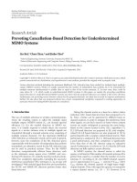
Crossed dipoles are shown in Figure 1. Each dipole in the ar-
ray is a short dipole, so the output voltage from each dipole
2 EURASIP Journal on Advances in Signal Processing
X
Z
Y
Figure 1: The structure of polarization sensitive array.
is proportional to the electric field component along that
dipole. There are orthogonal short dipoles, the x-andy-axis
dipoles, parallel to the x-andy-axes, respectively. The mth
dipole pair, m
= 1, 2, , M, has its center on the y-axis at
y
= (m − 1)d. The distance d between two adjacent dipole
pairs is assumed to be a half-wavelength to avoid angle ambi-
guity problems. We consider signals in the far-field, in which
case the signal sources are far enough away that the arriving
waves are essentially planes over the length of the array. As-
sume that the noise is independent of the source, and noise
is additive i.i.d. Gaussian.

2.1. The received signal model for polarization
sensitive antenna
We begin by considering the polarization of an incoming sig-
nal. Supposing that an antenna is at the origin of a spherical
coordinate system, and a signal b(t) is arriving from direc-
tion θ, ϕ,whereϕ is the elevation angle and θ is the azimuth
angle. Let this signal be a transverse electromagnetic (TEM)
wave, and consider the polarization ellipse produced by the
electric field in a fixed transverse plane. Polarization param-
eters are γ, η. We characterize the antenna in terms of its re-
sponse to linearly polar ized signals in the x and y directions.
Let v
x
be the complex voltage induced at the antenna out-
put terminals by an incoming electromagnetic signal with a
unit electric field polarized entirely in the x direction. Sim-
ilarly, let v
y
be the output voltages induced by signals with
unit electric fields polarized in the y directions. According to
[4], the total output voltage from polarization antenna is
y
p
(t) =

cos θ cos ϕ − sin ϕ
cos θ sinϕ cos ϕ

sin γe
jη

cos γ

b(t) = sb(t),
(1)
where
s
=

cos θ cos ϕ − sin ϕ
cos θ sinϕ cos ϕ

sin γe
jη
cos γ

(2)
is the polarization vector, and it relates to polarization and
DOA information.
2.2. The received signal model for polarization
sensitive array
Assume that a signal b(t) arrives at the uniform linear array
with M pairs of crossed dipoles. The received signal of the
polarization sensitive array is shown as follows:
y(t)
=

s
T
, qs
T

, , q
M−1
s
T

T
b(t) = (a ⊗ s)b(t), (3)
where
⊗ is Kronecker product, s is the polarization vector,
a
= [1, q, , q
M−1
]
T
is the direction vector, q = e
− j2πdsin θ/λ
.
When K sources impinge the polarization sensitive array,
the received signal at the output of the polarization sensitive
array is
x
=

a
1
⊗ s
1
, a
2
⊗ s

2
, , a
K
⊗ s
K

B
T
,(4)
where a
i
and s
i
are the direction vector and polarization vec-
tor of the ith source, respectively, and B
= [b
T
1
, b
T
2
, , b
T
K
]is
the source mat rix with N
× K,whereb
i
is the transmit signal
of the ith source.

Equation (4)canbedenotedas
x
= [A ◦ S]B
T
,(5)
where A
◦ S is Khatri-Rao product, A = [a
1
, a
2
, , a
K
] is the
direction matrix, and S
= [s
1
, s
2
, , s
K
] is the polarization
matrix.
Equation (5)canbedenotedas
x
=
⎡
⎢
⎢
⎢
⎢

⎣
X
··1
X
··2
.
.
.
X
··M
⎤
⎥
⎥
⎥
⎥
⎦
=
⎡
⎢
⎢
⎢
⎢
⎣
SD
1
(A)
SD
2
(A)
.

.
.
SD
M
(A)
⎤
⎥
⎥
⎥
⎥
⎦
B
T
,(6)
where D
m
(·) is understood as an operator that extracts the
mth row of its matrix argument and constructs a diagonal
matrix out of it, D
m
(A) = diag([a
m,1
, a
m,2
, , a
m,K
]).
Use slices to denote
X
··m

= SD
m
(A)B
T
, m = 1, 2, , M,(7)
where X
··m
is the mth slice in spatial direction.
In the presence of noise, the received signal model be-
comes

X
··m
=X
··m
+V
··m
=SD
m
(A)B
T
+V
··m
, m = 1, 2, , M,
(8)
where V
··m
, the 2 × N matrix, is the received noise corre-
sponding to the mth slice.
The signal in (7) is also denoted through rearrangements

as
x
m,n,p
=
K

f =1
a
m, f
s
n, f
b
p, f
, m = 1, , M;
n
= 1, , N; p = 1, 2,
(9)
X. Zhang and D. Xu 3
where a
m, f
stands for the (m, f )elementofA matrix, and
similarly for the others. Note that (9) is a sum of triple prod-
ucts; it is well known as the trilinear model, trilinear de-
composition, canonical decomposition, or PARAFAC analy-
sis. The trilinear model X reflects three different kinds of di-
versities available: spatial, temporal, and polarization diver-
sities. Another view, X
··m
= SD
m

(A)B
T
, m = 1, 2, , M,can
be interpreted as slicing the 3D data in a series of slices (2D
data) along the spatial direction. The symmetry of the trilin-
ear model in (9) allows two more matrix system rearrange-
ments, which can be interpreted as slicing the three-way data
along different directions. In particular,
Y
··p
= BD
p
(S)A
T
, p = 1, 2, (10)
where the N
× M matrix Y
··p
= [x
·,·,p
]. Y
··p
is the pth slice
in polarization direction. Similarly,
Z
··n
= AD
n
(B)S
T

, n = 1, 2, , N, (11)
where the M
× 2matrixZ
··n
= [x
n,·,·
]. Z
··n
is the nth slice in
the temporal direction.
3. BLIND PARAFAC SIGNAL DETECTION FOR
POLARIZATION SENSITIVE ARRAY
3.1. Trilinear alternating least squares
Trilinear alternating least square (TALS) algorithm is the
common data detection method for trilinear model [6]. The
basicideaofTALSisasfollows:(a)eachtime,updateama-
trix using least squares conditioned on previously obtained
estimates of the remaining matrix; (b) proceed to update an-
other matrix; (c) repeat until convergence. TALS algorithm is
discussed in detail as follows.
According to (6), least squares fitting is
min
A,S,B












⎡
⎢
⎢
⎢
⎢
⎢
⎣

X
··1

X
··2
.
.
.

X
··M
⎤
⎥
⎥
⎥
⎥
⎥
⎦

−
⎡
⎢
⎢
⎢
⎢
⎣
SD
1
(A)
SD
2
(A)
.
.
.
SD
M
(A)
⎤
⎥
⎥
⎥
⎥
⎦
B
T












F
, (12)
where
·
F
stands for the Frobenius norm.

X
··m
, m =
1, 2, , M, are the noisy slices.
Least squares update for B is

B
T
=
⎡
⎢
⎢
⎢
⎢
⎢

⎣

SD
1
(

A)

SD
2
(

A)
.
.
.

SD
M
(

A)
⎤
⎥
⎥
⎥
⎥
⎥
⎦
+

⎡
⎢
⎢
⎢
⎢
⎢
⎣

X
··1

X
··2
.
.
.

X
··M
⎤
⎥
⎥
⎥
⎥
⎥
⎦
, (13)
where [
·]
+

stands for pseudoinverse.

A and

S denot e previ-
ously obtained estimates of A and S.
Similarly, from the second way of slices, Y
··p
=
BD
p
(S)A
T
, p = 1, 2, which is rewritten as

Y
··1
Y
··2

=

BD
1
(S)
BD
2
(S)

A

T
, (14)
LS fitting is
min
A,S,B







Y
··1

Y
··2

−

BD
1
(S)
BD
2
(S)

A
T






F
, (15)
and the LS update for A is

A
T
=


BD
1
(

S)

BD
2
(

S)

+


Y
··1


Y
··2

. (16)
Finally, from the third way of slices, Z
··n
= AD
n
(B)S
T
, n =
1, 2, , N. And then LS update for S is

S
T
=
⎡
⎢
⎢
⎢
⎢
⎢
⎣

AD
1
(

B)


AD
2
(

B)
.
.
.

AD
N
(

B)
⎤
⎥
⎥
⎥
⎥
⎥
⎦
+
⎡
⎢
⎢
⎢
⎢
⎢
⎣


Z
··1

Z
··2
.
.
.

Z
··N
⎤
⎥
⎥
⎥
⎥
⎥
⎦
. (17)
The loss function to be minimized is the sum of squared
residuals (SSR) in the TALS algorithm:
SSR
=
M

m=1
N

n=1

2

p=1
e
2
m,n,p
, (18)
where e
m,n,p
= x
m,n,p
−

K
f =1
a
m, f
s
n, f

b
p, f
is the (m, n, p) ele-
ment of fitting error.
a
m, f
stands for the (m, f )elementof

A,
and similarly for the others.

According to (13), (16), and (17), matrices B, A,andS
are updated with conditioned least squares, respectively. The
matrix update will stop until convergence.
TALS is optimal when noise is additive i.i.d. Gaussian
[18]. TALS algorithm has several advantages: it is easy to
implement, guarantee to converge, and simple to extend to
higher order data. TALS algorithm is known to suffer from
degeneracy and slow convergence. Although a unique solu-
tion exists, it is not always guaranteed to be found as the
TALS algorithm can be stuck in local minima [19]. TALS
can be initialized by eigen-decomposition to speed up con-
vergence [12]. According to (10), the two slices along the po-
larization direction are represented as
Y
··1
= BA
E
, Y
··2
= BDA
E
, (19)
where A
E
= D
1
(S)A
T
and D = D
2

(S)D
1
(S)
−1
.
Construct auto- and c ross-correlation matrices:
R
1
= Y
H
··1
Y
··1
= A
H
E
B
H
BA
E
,
R
2
= Y
H
··1
Y
··2
= A
H

E
B
H
BDA
E
.
(20)
Define α
= A
H
E
B
H
B, then
R
1
= αA
E
, R
2
= αDA
E
. (21)
According to (21),
α
+
R
1
= D
−1

α
+
R
2
, (22)
4 EURASIP Journal on Advances in Signal Processing
where [·]
+
is the pseudoinverse. Let u
H
f
be the f th row of α
+
and let λ
f
be the f th element along the diagonal of D
−1
.The
general eigen-decomposition for (R
1
, R
2
)isgivenas
u
H
f

R
1
− λ

f
R
2

=
0, f = 1, 2, , K. (23)
The λ
f
’s and u
H
f
’s are the generalized eigenvalues and left
generalized eigenvectors of (R
1
, R
2
). Once α
+
is recovered,
then A
E
= α
+
R
1
, B = Y
··1
[A
E
]

+
,andD = B
+
Y
··2
[A
E
]
+
.
3.2. Identifiablity
The k-rank concept is very important in the trilinear algebra.
Definition 1 (see [10]). Consider a matrix A
∈ C
I×J
.If
rank(A)
= r, then A contains a collection of r linearly inde-
pendent columns. Moreover, if every l
≤ J columns of A are
linearly independent, but this does not hold for every l +1
columns, then A has k-rank k
A
= l. Note that k
A
≤ rank(A),
for all A.
Theorem 1 (see [20]). X
··m
= SD

m
(A)B
T
, m = 1, 2, , M,
where A
∈ C
M×K
, S ∈ C
2×K
,andB ∈ C
N×K
, considering that
A is a matrix with Vandermonde characteristic. If
k
S
+min

M + k
B
,2K

≥
2K + 2, (24)
then A, B, and S are unique up to permutation and scaling of
columns, that is to say, any other triple
A, B, S that const ructs
X
··m
(m = 1, 2, , M)isrelatedtoA, B,andS via
A = AΠΔ

1
, B = BΠΔ
2
, S = SΠΔ
3
, (25)
where Π is a per mutation matrix, and Δ
1
, Δ
2
,andΔ
3
are di-
agonal scaling matrices satisfying
Δ
1
Δ
2
Δ
3
= I. (26)
Scale ambiguity and p ermutation ambiguity are inherent
to the separation problem. This is not a major concern. Per-
mutation ambiguity can be resolved by resorting to a priori
or embedded information. The scale ambiguity can be re-
solved using automatic gain control and differential encod-
ing/decoding [21] or embedded information.
Although the PARAFAC uniqueness result is purely de-
terministic, it also admits statistical characteristics. A ma-
trix whose columns are drawn independently from an abso-

lutely continuous distribution has full rank with probability
one, even when the elements across a given column are de-
pendent random variables [11]. In our present context, for
source-wise independent source signals, k
B
= min(N, K); for
source-wise independent polarization, k
S
= min(2, K), and
therefore, (24)becomes
min(2, K)+min

M +min(N, K), 2K

≥
2K +2. (27)
In practice, K
≥ 2, min(2, K) = 2, hence the practical condi-
tion is
M +min(N, K)
≥ 2K. (28)
If N
≤ K, the identifiable condition is M + N ≥ 2K.
If N
≥ K, the identifiable condition is M ≥ K, and then
min(M, N) sources can be recovered.
If matrix A in Theorem 1 is not a Vandermonde matrix,
according to [11], the identifiable condition is
min(2, K)+min(N, K)+min(M, K)
≥ 2K +2. (29)

In practice, K
≥ 2, then the identifiable condition is
N
≥ K, M ≥ K, (30)
so min(M, N) sources can be recovered [8, 22, 23].
4. SIMULATION RESULTS
If X is the received signal without noise and

X = X + V is the
received noisy signal, we define the sample SNR as
SNR
= 10 log
10
X
2
F
V
2
F
dB, (31)
where
X
2
F
is the sum of squares of all elements of the 3D
data X.
As shown in Theorem 1, the scaling ambiguity and the
permutation ambiguity are inherent to this blind separation
problem. We remove the scaling ambiguity among the esti-
mated source matrix via embedded information. Permuta-

tion ambiguity is resolved using a greedy least square match-
ing algorithm [11].
A uniform linear array with 16 pairs of crossed dipoles
is used in the simulation. Assume that each source only has
one path to polarization sensitive array. We assume binary
phase-shift keying (BPSK) modulated signal and additive
gauss white noise. For all the simulation, the number of the
sources is 3. Note that N is the number of snapshots.
We present Monte Carlo simulations that are to assess
the bit error rate (BER) performance of the proposed blind
PARAFAC signal detection algorithm. The number of Monte
Carlo trials is 1000. The PARAFAC algorithm does not re-
quire DOA information and polarization information. We
compare our PARAFAC algorithm with the nonblind MMSE
receiver. MMSE receiver offers a performance bound against
which blind algorithms are often measured [24, 25]. For the
received signal in (5), the nonblind MMSE solution is

B
T
MMSE
=

ΛΛ
H
+
1
SNR

−1

Λ
H
x,whereΛ = A ◦ S.
(32)
Compared with our blind PARAFAC receiver, the nonblind
MMSE receiver assumes the perfect know ledge of DOA,
SNR, and polarization information.
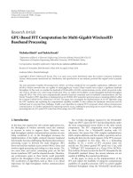
The performances of these algorithms under different N
are shown in Figures 2–7.
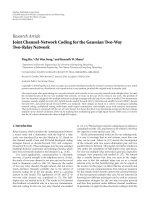
Figures 2 and 3 present large sample results for N
= 800
and N
= 400, respectively. From Figures 2 and 3,wefind
that blind PARAFAC signal detection algorithm is very close
to nonblind MMSE method.
X. Zhang and D. Xu 5
Blind PARAFAC receiver
Nonblind MMSE receiver
−8−10 −6 −4 −20 2
SNR (dB)
10
−6
10
−5
10
−4
10
−3
10
−2

10
−1
10
0
BER
Figure 2: The algorithm performances comparison with N = 800.
Blind PARAFAC receiver
Nonblind MMSE receiver
−8−10 −6 −4 −20 2 4
SNR (dB)
10
−5
10
−4
10
−3
10
−2
10
−1
10
0
BER
Figure 3: The algorithm performances comparison with N = 400.
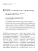
Figures 4 and 5 depict results for N = 200 and 100, re-
spectively. From Figures 2 to 5, we find that the gap between
blind PARAFAC and (nonblind) MMSE increases as N de-
creases.
Figures 6 and 7 show small sample results for N
= 50 and

N
= 20, respectively. It is clear that PARAFAC performs well
even for very small sample sizes.
The actual array parameters may differ from the nominal
array in several ways: gain, phase, and sensor location errors.
Gain and phase errors occur when the response of each
antenna to a known signal has a different amplitude and/or
phase response than expected. Blind PARAFAC signal detec-
tion algorithm performance in the array error condition is
also investigated. In this simulation, array error vector is the
Blind PARAFAC receiver
Nonblind MMSE receiver
−8−10 −6 −4 −20 2 4
SNR (dB)
10
−5
10
−4
10
−3
10
−2
10
−1
10
0
BER
Figure 4: The algorithm performances comparison with N = 200.
Blind PARAFAC receiver
Nonblind MMSE receiver

−8−10 −6 −4 −20 2 4 6
SNR (dB)
10
−6
10
−5
10
−4
10
−3
10
−2
10
−1
10
0
BER
Figure 5: The algorithm performances comparison with N = 100.
array gain and phase error vector. The array error vector g =
[0.8523 + 0.3031, 0.6071 − 0.4953i,0.7083 + 0.7059i,0.7497−
0.7167i,0.6931 + 0.8916i,0.8343 + 0.6883i,0.730 +
0.6894i,0.6678
− 0.5133i,0.4806 − 0.9112i,0.6669 +
0.5634i,0.7834
− 0.6828i,0.7497 − 0.7237i,0.6563 +
0.82316i,0.8123+0.6823i,0.7245+0.6239i,0.6234
−0.5133i].
Assume that array response vector for DOA
= θ is a(θ), then
the array response vector with array error is diag(g)a(θ).

The direction matrix with array error is not Vandermonde
matrix, and then the identifiable condition is shown in (30).
ThesamplenumberN is 100 in this simulation. The perfor-
mance of blind PARAFAC signal detection algorithm in array
error condition is shown in Figure 8. Figure 8 shows that
blind PARAFAC signal detection algorithm has the better
6 EURASIP Journal on Advances in Signal Processing
Blind PARAFAC receiver
Nonblind MMSE receiver
−8−10 −6 −4 −20 2 4 6 8
SNR (dB)
10
−6
10
−5
10
−4
10
−3
10
−2
10
−1
10
0
BER
Figure 6: The algorithm performances comparison with N = 50.
Blind PARAFAC receiver
Nonblind MMSE receiver
−8−10 −6 −4 −20 24 6 810

SNR (dB)
10
−5
10
−4
10
−3
10
−2
10
−1
10
0
BER
Figure 7: The algorithm performances comparison with N = 20.
performance in the array error condition. Blind PARAFAC
signal detection algorithm has robust characteristics to array
error.
5. CONCLUSIONS
This paper has developed a link between PARAFAC analy-
sis and blind signal detection for polarization sensitive array.
Relying on the uniqueness of low-rank three-way array de-
composition and trilinear alternating least squares, a deter-
ministic PARAFAC signal detection algorithm has been pro-
posed. The algorithm does not require DOA information and
polarization information, and it has blind and robust charac-
teristics. The simulation results reveal that the performance
PARAFAC receiver w ith array error
PARAFAC receiver with ideal array
−8−10 −6 −4 −20 2 4 6

SNR (dB)
10
−5
10
−4
10
−3
10
−2
10
−1
10
0
BER
Figure 8: The algorithm performance with array error.
of blind PARAFAC signal detection algorithm for polariza-
tion sensitive array is close to nonblind MMSE method, and
this algorithm works well in array error condition and sup-
ports small sample sizes.
ACKNOWLEDGMENTS
This work is supported by the startup fund of Nanjing Uni-
versity of Aeronautics and Astronautics (S0583-041) and
Jiangsu NSF Grant BK2003089. The authors wish to thank
the anonymous reviewers for valuable suggestions on im-
proving this paper.
REFERENCES
[1] J. W. P. Ng and A. Monikas, “Polarisation-sensitive array
in blind MIMO CDMA system,” Electronics Letters, vol. 41,
no. 17, pp. 970–972, 2005.
[2] I. Kaptsis and K. G. Balmain, “Base station polarization-

sensitive adaptive antenna for mobile radio,” in Proceedings of
the 3rd Annual International Conference on Universal Personal
Communications (ICUPC ’94), pp. 230–235, San Diego, Calif,
USA, September-October 1994.
[3]A.J.WeissandB.Friedlander,“Maximumlikelihoodsignal
estimation for polarization sensitive arrays,” IEEE Transactions
on Antennas and Propagation, vol. 41, no. 7, pp. 918–925, 1993.
[4] X. Zhenhai, W. Xuesong, X. Shunping, and Z. Zhuang, “Fil-
tering performance of polarization sensitive array: completely
polarized case,” Acta Electronica Sinica,vol.32,no.8,pp.
1310–1313, 2004.
[5] A. Smilde, R. Bro, and P. Geladi, Multi-Way Analysis. Applica-
tions in the Chemical Scie nces , John Wiley & Sons, Chichester,
UK, 2004.
[6] R. A. Harshman, “Foundations of the PARAFAC procedure:
model and conditions for an ‘explanatory’ multi-mode factor
analysis,” UCLA Working Papers Phonetics, vol. 16, no. 1, pp.
1–84, 1970.
X. Zhang and D. Xu 7
[7] J. D. Carroll and J J. Chang , “Analysis of individual differences
in multidimensional scaling via an n-way generalization of
“Eckart-Young” decomposition,” Psychometrika, vol. 35, no. 3,
pp. 283–319, 1970.
[8] L. De Lathauwer, B. De Moor, and J. Vandewalle, “Compu-
tation of the canonical decomposition by means of a simul-
taneous generalized Schur decomposition,” SIAM Journal on
Matrix Analysis and Applications, vol. 26, no. 2, pp. 295–327,
2004.
[9] L. De Lathauwer, “A link between the canonical decomposi-
tion in multilinear algebra and simultaneous matrix diago-

nalization,” SIAM Journal on Matrix Analysis and Applications,
vol. 28, no. 3, pp. 642–666, 2006.
[10] J. B. Kruskal, “Three-way arrays: rank and uniqueness of tri-
linear decompositions, with application to arithmetic com-
plexity and statistics,” Linear Algebra and Its Applications,
vol. 18, no. 2, pp. 95–138, 1977.
[11] N. D. Sidiropoulos, G. B. Giannakis, and R. Bro, “Blind
PARAFAC receivers for DS-CDMA systems,” IEEE Transac-
tions on Signal Processing, vol. 48, no. 3, pp. 810–823, 2000.
[12] N. D. Sidiropoulos, R. Bro, and G. B. Giannakis, “Parallel fac-
tor analysis in sensor array processing,” IEEE Transactions on
Signal Processing, vol. 48, no. 8, pp. 2377–2388, 2000.
[13] Y. Rong, S. A. Vorobyov, A. B. Gershman, and N. D. Sidiropou-
los, “Blind spatial signature estimation via time-varying user
power loading and parallel factor analysis,” IEEE Transactions
on Signal Processing, vol. 53, no. 5, pp. 1697–1710, 2005.
[14] Y. Yu and A. P. Petropulu, “Parafac based blind estimation
of MIMO systems with possibly more inputs than outputs,”
in Proceedings of IEEE International Conference on Acoustics,
Speech, and Signal Processing (ICASSP ’06), vol. 3, pp. 133–136,
Toulouse, France, May 2006.
[15] K. N. Mokios, N. D. Sidiropoulos, and A. Potamianos, “Blind
speech separation using parafac analysis and integer least
squares,” in Proceedings of IEEE International Conference on
Acoustics, Speech, and Signal Processing (ICASSP ’06), vol. 5,
pp. 73–76, Toulouse, France, May 2006.
[16] X. Zhang and D. Xu, “Blind PARAFAC receiver for space-time
block-coded CDMA system,” in Proceedings of International
Conference on Communications, Circuits and Systems, vol. 2,
pp. 675–678, Guilin, Guangzi, China, June 2006.

[17] X. Zhang and D. Xu, “PARAFAC multiuser detection for
SIMO-CDMA system,” in Proceedings of International Confer-
ence on Communications, Circuits and Systems, vol. 2, pp. 744–
747, Guilin, Guangzi, China, June 2006.
[18] S. A. Vorobyov, Y. Rong, N. D. Sidiropoulos, and A. B. Ger-
shman, “Robust iterative fitting of multilinear models,” IEEE
Transactions on Signal Processing, vol. 53, no. 8, part 1, pp.
2678–2689, 2005.
[19] G. Tomasi and R. Bro, “A comparison of algorithms for fitting
the PARAFAC model,” Computational Statistics & Data Anal-
ysis, vol. 50, no. 7, pp. 1700–1734, 2006.
[20] N. D. Sidiropoulos and X. Liu, “Identifiability results for
blind beamforming in incoherent multipath with small delay
spread,” IEEE Transactions on Signal Processing, vol. 49, no. 1,
pp. 228–236, 2001.
[21] J. G. Proakis, Digital Communications,McGraw-Hill,New
York, NY, USA, 3rd edition, 1995.
[22] S. E. Leurgans, R. T. Ross, and R. B. Abel, “A decomposition
for three-way arrays,” SIAM Journal on Matrix Analysis and
Applications, vol. 14, no. 4, pp. 1064–1083, 1993.
[23] E. Sanchez and B. R. Kowalski, “Tensorial resolution: a di-
rect trilinear decomposition,” Journal of Chemometrics, vol. 4,
no. 1, pp. 29–45, 1990.
[24] D. Gesbert, J. Sorelius, and A. Paulraj, “Blind multi-user
MMSE detection of CDMA signals,” in Proceedings of IEEE
International Conference on Acoustics, Speech, and Signal Pro-
cessing (ICASSP ’98), vol. 6, pp. 3161–3164, Seattle, Wash,
USA, May 1998.
[25] M. K. Tsatsanis and Z. Xu, “Performance analysis of minimum
variance CDMA receivers,” IEEE Transactions on Signal Pro-

cessing, vol. 46, no. 11, pp. 3014–3022, 1998.
Xiaofei Zhang received the M.S. degree in
electrical engineering from Wuhan Univer-
sity, Wuhan, China, in 2001. He received the
Ph.D. degree in communication and infor-
mation systems from Nanjing University of
Aeronautics and Astronautics in 2005. From
2005 to 2007, he was a Lecturer in Electronic
Engineering Department, Nanjing Univer-
sity of Aeronautics and Astronautics, Nan-
jing, China. His research is focused on array
signal processing and communication signal processing.
Dazhuan Xu graduated from Nanjing Insti-
tute of Technology, Nanjing, China, in 1983.
He received the M.S. and Ph.D. degrees in
communication and information systems
from Nanjing University of Aeronautics and
Astronautics in 1986 and 2001, respectively.
He is now a Full Professor in the College of
Information Science and Technology, Nan-
jing University of Aeronautics and Astro-
nautics, Nanjing, China. His research inter-
ests include digital communications, software radio, coding theory,
and medical signal processing.