Báo cáo hóa học: " Research Article GPU-Based FFT Computation for Multi-Gigabit WirelessHD Baseband Processing" pptx

Hindawi Publishing Corporation
EURASIP Journal on Wireless Communications and Networking
Volume 2010, Article ID 359081, 13 pages
doi:10.1155/2010/359081
Research Article
GPU-Based FFT Computation for Multi-Gigabit WirelessHD
Baseband Processing
Nicholas Hinitt
1
and Taskin Kocak
2
1
Department of Electric & Electronic Engineering, University of Bristol, Bristol, BS8 1UB, UK
2
Department of Computer Engineering, Bahcesehir University, 34538 Istanbul, Turkey
Correspondence should be addressed to Taskin Kocak,
Received 13 November 2009; Revised 19 May 2010; Accepted 29 June 2010
Academic Editor: Mustafa Badaroglu
Copyright © 2010 N. Hinitt and T. Kocak. This is an open access article distributed under the Creative Commons Attribution
License, which permits unrestricted use, distribution, and reproduction in any medium, provided the original work is properly
cited.
The next generation Graphics Processing Units (GPUs) are being considered for non-graphics applications. Millimeter wave
(60 Ghz) wireless networks that are capable of multi-gigabit per second (Gbps) transfer rates require a significant baseband
throughput. In this work, we consider the baseband of WirelessHD, a 60 GHz communications system, which can provide a data
rate of up to 3.8 Gbps over a short range wireless link. Thus, we explore the feasibility of achieving gigabit baseband throughput
using the GPUs. One of the most computationally intensive functions commonly used in baseband communications, the Fast
Fourier Transform (FFT) algorithm, is implemented on an NVIDIA GPU using their general-purpose computing platform called
the Compute Unified Device Architecture (CUDA). The paper, first, investigates the implementation of an FFT algorithm using
the GPU hardware and exploiting the computational capability available. It then outlines the limitations discovered and the
methods used to overcome these challenges. Finally a new algorithm to compute FFT is proposed, which reduces interprocessor
communication. It is further optimized by improving memory access, enabling the processing rate to exceed 4 Gbps, achieving a

processing time of a 512-point FFT in less than 200 ns using a two-GPU solution.
1. Introduction
As the data rates required for rich content applications rise,
the throughput of wireless networks must also continue
to increase in order to support them. Therefore, very
high throughput wireless communications systems are now
being considered [1–4]. As the throughput increases, the
implementation of the highly compute intensive baseband
functionality becomes challenging. Baseband (physical layer)
processing occurs in between the radio frequency (RF)
front-end and the medium access control (MAC) layer, and
involves signal processing and coding on a data stream. The
two most time and power consuming parts are the fast
fourier transform (FFT) and the channel decoder. Therefore,
any performance gains in these blocks could potentially
improve the throughput of the whole system significantly.
The acceleration of algorithms such as these is of critical
importance for high throughput wireless communications
systems.
The 3.8 Gbps throughput required by the WirelessHD
“high-rate PHY” places the FFT and decoding blocks under
the most computational strain relative to the other system
components. The FFT computation must be completed
in about 200 ns. For a WirelessHD modem with 512
subcarriers, this means that 2304 complex multiplications,
4608 complex additions and the ancillary operations such as
loading the data into the input registers of the FFT processor
must be completed in that time. This is a demanding
deadline. In [5], a review of FFT execution times was
carried out. The fastest quoted FFT speed was 5.5 μs, with

a “DSPlogic” FFT instantiated on a Virtex-II Pro 50 FPGA.
This is about 28 times too slow for the FFT demanded by the
WirelessHD standard. Hence, the current solutions are not
capable of fulfilling the required specification.
In this paper, we focus on the implementation of the
FFT and explore the feasibility of using the computational
capability of a graphics processor (GPU) to achieve gigabit
baseband throughput using the WirelessHD specification
2 EURASIP Journal on Wireless Communications and Networking
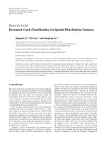
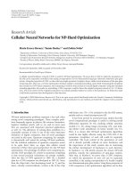
CPU GPU
CPU or GPU core
On-chip cache
Figure 1: An illustration of the differences between CPUs and
GPUs.
[6]. GPU is a massively parallel device, with a significant
number of processing cores, whose processing ability can be
exploited for general purpose use in high arithmetic intensity
algorithms, where the parallel nature of its architecture can
be exploited to maximum benefit. The NVIDIA compute
unified device architecture (CUDA) platform [7] is used in
order to access the computational capability provided by the
GPU, which enables a programmer to utilize the parallel
processing functionality of NVIDIA GPUs. The details of the
GPU used in this paper are discussed in the following section.
There is a growing number of recently reported works on
implementations of various applications on general-purpose
GPU (GPGPU) technology [8]. To cite a few, in [9], the
authors discuss the implementation of an image processing
application using GPU. A MapReduce, a distributed pro-
gramming framework originally proposed by Google for the

ease of development of web search applications on a large
number of commodity CPUs, framework is developed on a
GPU in [10]. GPUs are used to accelerate the computational
intensive operations in cryptographic systems [11]. The
authors in [12] also use GPUs to accelerate radiative heat
transfer simulation for a large form factor matrix. Accel-
eration of molecular modeling applications with graphics
processors are presented in [13]. Authors in [14] discuss GPU
implementation of sequence alignment algorithms used in
molecular biology. Several other applications of general-
purpose processing using GPUs are covered in a recent
special issue [15].
There are also some reported FFT implementations on
GPUs. In [16], the authors proposed an implementation to
exploit the memory reference locality to optimize the parallel
data cache. The same authors also reported their experiences
with mapping nonlinear access patterns to memory in CUDA
programming environment [17]. The researchers in [18,
19] addressed computation-intensive tasks such as matrix
multiplication in implementing FFT on GPUs. In [20], the
authors presented algorithms for FFT computation based
on a Stockham formulation. Their algorithm attempts to
optimize the radix with respect to the threads and the
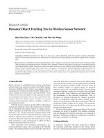
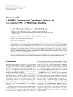
SP SP
SP SP
SP SP
SP SP
Instruction unit
SFU SFU
Shared memory

Figure 2: Streaming multiprocessors in detail.
registers available to them. Their work, like ours, tries
to use the memory and registers efficiently to increase
the performance. In another paper by Govindaraju and
Manocha [21], the authors also use a Stockham-based FFT
algorithm for cache-efficient implementation.
Note that our aim is this work is not to come up with
the fastest FFT algorithm but rather come up with a design
that will accommodate FFT computation for the WirelessHD
standard. The algorithms in the literature aim for the fastest
implementation on the GPU and they do not take some
features, for instance, memory transfer, into account. For
example, in [20], it was specifically mentioned in Section 6.D,
where the authors discuss the limitations of their work, their
algorithm works only on data which resides in GPU memory.
They added when the data must be transferred between GPU
and system memory, the performance will be dramatically
lowered. Hence, a comparison between the results of this
paper (similarly others) and ours will not be an apple-to-
apple comparison. In order to emphasize our contributions,
though, we compare the original CuFFT algorithm with five
difference proposed enhancements as well as our proposed
FFT algorithm and also give GFLOPs performance for these.
Reference [21] is another paper in the literature, which may
seem similar to this work in the first instance; however, there
are many differences: theirs use Stockham FFT algorithm,
ours is based on Cooley-Tukey radix-2 FFT algorithm. They
literally focus on the cache-efficiency, our work attempts to
use the memory access efficiently but it does not go into
cache structures. They exploit the nested loops in numerical

algorithms, our algorithm exploits the fact that the butterfly
selections follow a pattern when computing the multipliers
in the FFT.
1.1. Contributions of This Paper. This paper makes several
contributions while exploring the feasibility of achieving
multigigabit baseband throughput.
EURASIP Journal on Wireless Communications and Networking 3
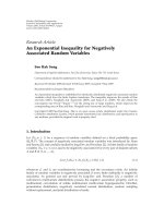
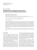
Device
Interconnection network
DRAM
Host
PCI express bus
Host memory
Figure 3: An overview of the GPU architecture.
(1) A new algorithm for FFT computation is proposed.
By grouping the butterfly operations, the proposed
algorithm reduces the number of interprocessor
communications. This leads into reducing the num-
ber of shared-memory accesses and hence eventually
reducing the overall FFT computation time.
(2) New load and save structures are proposed to
improve the shared memory access. The order of
accesses to the shared memory is modified to increase
the amount of read and write coalescing. This has a
significant impact on the algorithm performance.
(3) New data types and conversions are developed. These
8-bit and 16-bit data types were not available in
the existing CUDA environment and are used to
overcome bandwidth limitations.
(4) Last but not least, it is shown that multigigabit FFT

computation can be achieved by software implemen-
tation on a graphics processor.
The rest of the paper is organized as follows. Section 2
gives an overview of the GPU used in this work. Section 3
describes the WirelessHD standard. CUDA FFT algorithm
and enhancements are covered in Section 4. The new FFT
algorithm is introduced in Section 5. Improvements for the
shared memory access are also presented in this section.
Finally, the paper concludes in Section 6.
2.TheGraphicsProcessor
Most central processing units (CPUs) now have between 2
and 4 cores, serviced by varying amounts of on-chip cache
as shown in Figure 1. The GPUs used in this work have 24
streaming multithreaded processors (SM) each with 8 cores,
giving 192 cores in total. Each SM has a limited amount of
cache known as shared memory which is accessible by all
eight cores. Whilst the GPU cores are much less versatile
than the CPU cores, and are clocked at lower frequencies,
the combined processing capability for well designed parallel
algorithms can easily exceed the capability of a CPU. This
explains the emergence of the GPGPU technology for high
performance applications.
2.1. Hardware: A Closer Look. The NVIDIA GPU architec-
ture is constructed around SM processors. These consist of
8 scalar processors (SP), two special function units (SFU),
a multithreaded instruction unit and a block of shared
memory, as seen in Figure 2. Each GTX260 GPU used in
this work has 24 SMs, each of which can run 1024 threads
concurrently, so each SP handles 128 threads, giving a total
of 24,576 threads per GPU. This vast amount of processing

power is supported by a large amount of global memory.
This is off-chip memory located on the GPU main board,
primarily used to store data prior to and after calculation. A
CUDA kernel call specifies the number of blocks, and threads
per block, that must be processed. All the threads of a given
block must execute on the same SM and as a block completes
another will be scheduled if there are remaining blocks to be
computed. Only one kernel may execute at any one time.
Thread execution is implemented using a single instruc-
tion multiple thread (SIMT) architecture, where each SP
executes threads independently. Threads are executed in
parallel, in groups of 32 consecutive threads, called warps.
Every instruction time, a warp that is ready to execute is
selected and the same instruction is then issued to all threads
of that warp, so maximum speed is obtained if there are
no divergent branches in the code. For example, in an “IF”
statement, if 17 threads follow one branch, and 15 the other,
the 17 are suspended and 15 execute, and then 17 execute
with the 15 suspended, so effectively both branches of the
“IF” statement are processed.
2.2. Compute Unified Device Architecture. The CUDA plat-
form is an extension of the C language which enables
the programmer to access GPU functionality for parallel
processing. It includes a set of additional function qualifiers,
variable type qualifiers and built in variables. These are
used to define and execute a kernel, a function called from
the Host (PC) and executed on the Device (GPU). These
functions are not written as explicitly parallel code, but the
Device hardware automatically manages the threads that run
in parallel.

The NVIDIA CUDA system uses an application pro-
gramming interface (API) [22] which hides the complex
architecture of the GPU. This hardware abstraction simplifies
the task of coding for the GPU, and also has the advantage
that the underlying architecture can change significantly
in future products and the code designed for an older
device will still work. The CUDA programming model [23]
4 EURASIP Journal on Wireless Communications and Networking
RF front end
Down conversion
Symbol shaping
Guard interval
FFT
Tone deinterleaver
Pilot remove
Symbol demapper
Bit deInterleaver
Data deMUX
Viterbi decoder
Outer
interleaver
Outer
interleaver
Descrambler
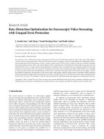
Figure 4: WirelessHD baseband receiver block diagram.
is based on a system where individual groups of threads
use their own shared memory and local registers, with
intermittent synchronization across all groups at defined
points within the code. Therefore, maximum performance
can be achieved if an algorithm is broken into sections that

are each independent, where the individual sections can then
be split into smaller divisions where data can be shared
between those divisions.
2.3. Memor y Access. Every CUDA thread may access several
types of memory, each of which has a different access speed.
The fastest is the thread level register space, which at full
occupancy is limited to 16 registers per thread, although at
maximum 32 are available. Occupancy is a measure of the
number of active threads relative to the maximum number of
threads that can be active for the given GPU and it is affected
by the memory usage of threads and blocks. The next fastest
is the shared memory, which is accessible by all the threads
of a single block, of which there is a limit of 8 Kbytes per
block at full occupancy, or a maximum of 16 Kbytes. The
slowest access speed is for the global memory, of which for
the GTX260s used in this project there is 896 Mbytes, which
is accessible by all threads. In addition to this, there is another
memory space which is read-only for the Device, known as
4
4.5
5
5.5
6
6.5
7
7.5
FFT processing time (us)
128 512 2048 8192 32768
Batch size
Figure 5: Graph showing the calculation time per FFT against batch

size.
the constant space, which the Host can copy data to, for
applications such as look up tables.
The global memory access speed is due to the DRAM
used being off chip, so although it is still on the GPU
mainboard, the latency can be up to a few hundred clock
cycles. This latency is hidden by the action of the thread
schedulers, such that if a thread is waiting for data it will
be de-scheduled and another is rescheduled. Once the data
transaction is complete the thread will be reinstated on the
list of threads to be processed. In this way, the vast number
of threads hides the effect seen by such memory latency.
The interconnect between the GPU and CPU is provided
by the PCI Express Bus, shown in Figure 3, which links the
Host memory with the Device global memory. Data required
for a kernel’s execution must be loaded on to Device memory
by the Host prior to the kernel being launched as the GPU
cannot access Host memory, nor instigate transfers to or
from it.
3. WirelessHD
WirelessHD aims to enable consumer devices to create a
wireless video area network (WVAN), for streaming High
Definition (HD) video with resolutions of up to 1080P, 24 bit
colour at 60 Hz, and also provide 5.1 surround sound audio.
This papre has focussed only on the high rate physical (HRP)
video link, as this is by far the most computationally intensive
section of the specification [6]. The HRP link uses OFDM to
achieve the 3.8 Gbps required for the streaming of the HD
video in an uncompressed format.
WirelessHD utilizes the unlicensed bandwidth in the

60 GHz region, with a typical range of 10 m. This is achieved
using smart antenna technology that adapts to environmen-
tal changes by focusing the receiver antenna in the direction
of the incoming power from the transmitter using beam
forming and steering. This enables both improvements in
the quality of the line of sight link and also enables use of
reflected paths if line of sight is not available.
There are many data, coding rates, and subcarrier
modulation schemes used in WirelessHD, depending on
the throughput required. The OFDM system outlined in
the WirelessHD specification [6] uses 512 subcarriers of
which 336 carry data, each modulated using 16 Quadrature
Amplitude Modulation (QAM).
EURASIP Journal on Wireless Communications and Networking 5
Stream 3
Stream 2
Stream 1
Stream 0
Time
Host—Device memory copy
Device—Host memory copy
Kernel execution
Figure 6: Illustration of streaming execution. This diagram assumes zero streaming overheads which would also affect performance.
Table 1: WirelessHD specification parameters [6].
Parameter Value
Occupied bandwidth 1.76 GHz
Reference sampling rate 2.538 Gsamples/second
Number of subcarriers 512
FFT period
∼201.73 ns

Subcarrier spacing
∼4.957 MHz
Guard interval
∼25.22 ns
Symbol duration
∼226.95 ns
Number of data subcarriers 336
Number of DC subcarriers 3
Number of pilots 16
Number of null subcarriers 157
Modulation QPSK, 16-QAM
Outer block code RS(224,216), rate 0.96
Inner code 1/3, 2/3 (EEP), 4/5, 4/7 (UEP)
Figure 7 illustrates the data transmission process. To
convert the N frequency domain symbols of each channel
into the time domain signal transmitted, an N-point inverse
FFT must be applied to the baseband signals of the N
subcarrier OFDM system. In the receiver, an N-point FFT is
used to switch from the time domain signal back to frequency
domain data which can then be quantised and decoded. For
WirelessHD, there are 2.538 giga samples per second using
512 sub carriers. Therefore, in the baseband of the receiver,
depicted in Figure 4, a 512-point FFT must be computed
every 226.95 ns in order to achieve a raw throughput of
5.9 Gbps. The key specifications for WirelessHD can be
found in Ta bl e 1 .
4. CUDA FFT Algorithm and Enhancements
In this section, we first utilize CuFFT [24], an FFT library
included in the CUDA software development kit (SDK),
to implement the FFT functionality required for the Wire-

lessHD standard. CuFFT provides a set of standard FFT
algorithms designed for the GPU. A benchmarking program
obtained on the NVIDIA CUDA forum was used to assess
the performance of this library. Minor modifications were
made to the code, to enable it to run on the test system.
An example CUDA FFT code is given in Figure 13 .The
execution of the algorithm is also discussed there. Tests
showed that a 512-point FFT would be calculated in 7 μs
with the original CuFFT code using a single GPU. Since this
time is not anywhere close to the required duration for the
FFT calculation, we explored several methods to enhance the
performance achieved by the CuFFT implementation. Below,
we will describe these methods.
4.1. Method #1: Using Large Batch Size. The batch size is
defined as the number of FFTs performed by the kernel in
a single execution. Analysis showed that as the batch size
increased, the processing time per FFT reduced towards the
minimum of 4.15 μs, shown in Figure 5. This shows that the
overheads in initializing the kernel become insignificant to
the execution time when the batch size rises above 8192 FFTs.
Allfuturecodeexecutionsusedabatchsizegreaterthan
16384 FFTs to eliminate the kernel overhead.
4.2. Method #2: Using Page-Locked Memory and Radix-2.
Host memory that is page-locked, also known as pinned
memory, ensures the assigned program memory is held in
physical memory and is guaranteed not to be written to the
paging file and removed from physical memory. This means
the page-locked memory can be accessed immediately, rather
than having to be restored from the paging file prior to access.
Using CUDA functionality, page-locked memory can

be allocated as well as the regular pageable memory. The
advantage of page-locked memory is that it enables a higher
bandwidth to be achieved between the Device and Host.
However, page-locked memory is a limited resource, and so
the programmer must limit its allocation. The page-locked
memory is also used by the computer operating system, so if
large amounts are allocated for use with CUDA, then overall
system performance may be affected, as it may force critical
memory to be written to the paging file. The FFT program
using the page-locked memory technique considered what
gains may be achieved by utilizing this additional bandwidth.
Given the available radix sources, the radix-2 algorithm
was the most appropriate for calculating a 512-point FFT.
The CUDA FFT radix-2 code is based on the Cooley-Tukey
algorithm, but the algorithm is parallelized such that there
6 EURASIP Journal on Wireless Communications and Networking
512 - 16 QAM transmitted data sets 512 - 16 QAM received data sets
IFFT FFT
Time domain transmitted signal
Figure 7: An illustration of the data transmission process.
Figure 8: Constellation diagram of 16-QAM showing 5-bit accu-
racy divisions.
are 256 threads per FFT, each executing a single butterfly for
each of the 9 stages of the 512-point FFT.
The performance gain of using page-locked memory and
explicit execution of the radix-2 CUDA FFT source was
analysed over a range of batch sizes. It was found that these
modifications offered a significant improvement in the FFT
calculation time, reducing it to 2.83 μs per FFT when using
16384 FFTs per batch.

4.3. Method #3: Asynchronous Concurrency. In order to
facilitate concurrent execution between the Host and the
Device, some Device functions can be called asynchronously
from the Host such that control is returned to the Host prior
to the Device completing the task assigned. Asynchronous
memory copies can be called to initiate Device-to-Host or
Host-to-Device copies whilst a kernel is executing.
Kernels manage concurrency through streams. A stream
is a sequence of operations which are processed in order;
however, different streams can execute out of order with
respect to one another. Since only one kernel is able to run on
the Device at any one time, a queue of streams can be formed
such that the memory copies of one stream can overlap with
the kernel execution of another stream as shown in Figure 6.
It should be noted that the memory copies themselves cannot
overlap if maximum bandwidth is to be provided in a single
copy, as all transfers utilize the same PCI Express Bus.
Asynchronous concurrency was implemented such that
a batch of FFTs was divided equally between the number
of available streams. Tests showed that in fact two streams
proved to be the most efficient, reducing the total compu-
tation time to 2.54 μs per FFT, and that batch size did not
affect the 2-stream performance. Whilst streams decreased
the calculation time by 290 ns, the overall performance
remained significantly above that required to provide a
gigabit throughput. This was due to the fact that the memory
transfer time was a limiting factor in the performance of the
algorithm, which streams cannot overcome.
4.4. Method #4: Reduced Accuracy for Input/Output Limi-
tations. The previous subsection highlighted a significant

challenge in the memory transfer limitations between the
Device and Host. In order to target a solution to this, it
was necessary to first consider why this was a performance
bottleneck.
In the WirelessHD HRP link specification each FFT
corresponds to 336 16-QAM data signals, equivalent to 1344
raw received bits. Using an outer code of rate 0.96 and inner
code of rate 2/3 this represents 860 decoded data bits. The
computation for this is achieved in 226.95 ns so fulfilling the
3.8 Gbps decoded data rate of the HRP link.
Decoded Data Rate
=
860
226.95 ×10
−9
= 3.8Gbps,
Raw Data Rate
=
1344
226.95 ×10
−9
= 5.95Gbps.
(1)
In a single FFT, 512 complex values must be copied to the
Device, computations take place and the results be copied
off again within the 226.95 ns deadline. When the memory
copies alone are considered, in full 32-bit accuracy this
requires an astounding bandwidth of 36 GBps
2
×

(
32
×2 ×512
)
226.95 ×10
−9
≈ 290Gbps ≈ 36GBps. (2)
This represents a 76.2 : 1 ratio, relative to the decoded data
rate. The reason for this bandwidth requirement is that the
FFT is calculated prior to quantization, using magnitude and
phase data from the receiver provided at a given accuracy.
The accuracy of the complex signals must be sufficient to be
able to mathematically separate the incoming signals into 16-
QAM data channels and nulls precisely, so that quantization
can occur.
EURASIP Journal on Wireless Communications and Networking 7
Table 2: Break down of calculation time.
Memory copy
time (μs)
Floating point
conversion
(μs)
Kernel call
overhead (μs)
Algorithm
performance
(μs)
1.024 0.603 0.0028 0.423
The maximum benchmarked bandwidth for the PCI
Express 1.0 bus on the motherboard used was 3.15 GBps.

Given this, even with a 2-GPU solution, full 32-bit accuracy
at gigabit data throughputs with the current hardware was
not achievable.
There are three ways to overcome the bandwidth issues.
Hardware Upgrade. A PCI Express 2.0 compliant mother-
board could be used.
Compression. Lossless compression could be employed to
reduce the data transfer size. However, the compres-
sion/uncompression will add to the already tight schedule for
the computation of the baseband algorithms in WirelessHD.
Reduced Accuracy Transfer . The majority of wireless commu-
nications systems use less than 16-bit accuracy and many less
than 8-bit accuracy and therefore the possibility of reducing
the accuracy of the data transferred between the Host and
Device was explored. Since the GPU generally performs
calculations in 32-bit floating point accuracy, additional
processing time was required to convert the data prior to and
post calculation.
4.4.1. Performance for the 16-Bit Reduced Accuracy Transfers.
The LittleFloat, a 16-bit floating-point data type was created
and integrated into the FFT code. It uses one sign bit,
5 exponent bits, and 10 mantissa bits. Tests showed the
reduction in Host-to-Device and Device-to-Host transfer
times had a significant impact on the calculation rate of the
algorithm. The fastest processing time of 1.34 μs per FFT
was achieved using 4 streams. Analysis was carried out to
provide a complete breakdown of the execution time and to
find the performance of the conversion algorithm in the FFT
calculation.
The tests undertaken to obtain this information are

shown below.
(i) Instigate the memory transfers, but exclude the FFT
kernel call.
(ii) Initiate memory transfers and also the kernel call but
the function to run the FFT calculation was omitted
so only the floating point conversions were processed.
(iii) Executed an empty kernel, to find the kernel execu-
tion overhead.
These tests were performed using a single stream to ensure
the effects of streaming would not hide any processing time.
TheresultsaregiveninTa ble 2.
Table 3: Break down of calculation time.
Memory copy
time (ns)
Floating point
conversion
(ns)
Kernel call
overhead (ns)
Algorithm
performance
(ns)
320 80 2.8 360
The conversion time was relatively significant, taking
300 ns per conversion. Whilst the single stream calculation
and conversion time took significantly longer than the
507 ns calculated earlier, streams almost completely hid this
additional time, such that the overall calculation time was a
few hundred nanoseconds above the memory transfer time.
4.4.2. Performance for the 8-Bit Reduced Accuracy Transfers.

Consideration was given to whether 8-bit accuracy was
sufficient for the FFT data. On a constellation diagram, 16-
QAM uses 16 points to identify the values of 4 data bits.
These are spaced equally about the origin in a grid, such that
each point is equidistant from its neighbours. Figure 8 shows
a 16-QAM constellation diagram with markers dividing the
distance between points into 8. This illustrates the number
of unique positions if 5-bit accuracy were used, giving 32
individual points on each row and column or 1024 individual
points in total.
If 8-bit accuracy were used there would be 65536 unique
points. Therefore it was determined that 8-bit accuracy
would be sufficient to represent the requested data.
If an 8-bit data accuracy system (TinyFixed) was imple-
mented it could reduce the transfer time such that it would
be comparable with the calculation time. However, this in
itself was not sufficient, the time taken for the floating point
conversion had to be reduced, as a single conversion to
or from the LittleFloat 16-bit data type exceeded the total
processing time required for the entire WirelessHD FFT
calculation.
Using a single stream, an FFT was calculated in 860 ns
including memory transfer time and float conversion, and
using 4 streams this was achieved in 534 ns. As the calculation
time now approached low hundreds of nanoseconds, it
became apparent that the use of streams added approx-
imately 100 ns to the total computation time. This was
verified by running the same program without any streaming
code. In this case, the total execution time was approximately
100 ns less than the single stream execution time. Given

that the total memory transfer took 320 ns, allowing for
the 100 ns streaming overhead, the single stream time
indicates calculation was achieved in 440 ns using the CUDA
FFT algorithm, including conversion time. The conversion
time of TinyFixed was significantly better than LittleFloat
achieving 40 ns per conversion, so computation alone took
approximately 360 ns. The calculation time breakdown is
tabulated in Tab le 3 .
The overall computation performance significantly
improved to 534ns per FFT on a single GPU. The balance of
calculation to memory transfer time was significantly closer
taking greater advantage of the functionality provided by
streams.
8 EURASIP Journal on Wireless Communications and Networking
G[k]
H[k]
e
−j
2πk
N
X[k]
X[k + N/2]
−
(a)
x[0]
x[2]
x[4]
x[6]
x[1]
x[3]

x[5]
x[7]
2-Point
FFT
2-Point
FFT
2-Point
FFT
2-Point
FFT
1
−j
1
−j
4-Point
FFT
4-Point
FFT
1
−j
2π
4
e
-j
−j
2π
4
e
X[0]
X[1]

X[2]
X[3]
X[4]
X[5]
X[6]
X[7]
(b)
Figure 9: (a) 2-point FFT and (b) The decomposition of a DIT 8-point radix-2 FFT.
Table 4: Performance summary of CuFFT and proposed methods
to improve it.
Method FFT time (μs)
CuFFT with no enhancements 7
CuFFT enhancement #1: 4.15
Large Batch Size
CuFFT enhancement #2: 2.83
Page-locked memory + radix-2
CuFFT enhancement #3: 2.54
Asynchronous concurrency (streaming)
CuFFT enhancement #4: 1.34
Reduced accuracy (16-bit)
CuFFT enhancement #5: 0.534
Reduced accuracy (8-bit)
4.5. Performance Summary of CuFFT and Proposed Enhance-
ments. We provide a summary of the performances achieved
by the original CuFFT and the proposed methods to improve
it in Tab le 4 . Though, there is a reduction in FFT time
with the addition of each enhancement, we still cannot fulfil
the WirelessHD specification. Therefore, it is necessary to
consider the development of a new algorithm.
5. A New FFT Algorithm

In order to get a better FFT performance, the new algorithm
needs to exploit the architecture of the GPU so as to
maximise the processing throughput. Consideration was
given to radix-8, and split-radix algorithms; however, the
fine grained nature of the radix-2 algorithm offered a
greater degree of flexibility than the other radices, as it
was unknown how many butterflies would best fit per
thread given the limited number of registers available.
Also, the additional complexity of these algorithms was
thought inappropriate given the scale of the parallelism
required in the implementation of a new algorithm on
the GPU. One of the limiting factors for performance
is the interprocessor communication. References [25, 26]
present implementations of the FFT without interprocessor
communications, showing how the performance of the FFT
could be enhanced significantly in avoiding communication
with other processors by loading the entire input data to the
processor. However, their direct application to the CUDA
platform was not possible due to the limited register space
available per thread. In this way, the CUDA architecture is
limited in that since the register space is very small, only 16
per thread, if full occupancy was to be achieved then such a
method could not be used. Nevertheless, the idea of limiting
interprocessor communications could be applied.
5.1. Algorithm Overview. Basically, in order to reduce the
interprocessor communications, our algorithm exploits the
fact that the butterfly selections follow a pattern when
computing the multipliers in the FFT. Limiting the inter-
processor communication is possible by grouping 4 butterfly
calculations into a single thread. If the correct butterflies are

chosen, within each thread 3 stages of calculation can be
implemented without interprocessor communication. Given
that for a radix-2, 512-point FFT there are 9 stages, using this
strategy, shared memory need only be accessed at two points
in the entire calculation (see Figure 10). All other accesses
within the calculation are to the internal thread registers,
which have inherent speed enhancements as these are the
fastest accesses. The details of the algorithms are given in the
following subsection.
5.2. Algorithm Development. An 8-point FFT can be rep-
resented by two 4-point FFTs and a set of butterflies, and
similarly the 4-point DFT can be seen as two 2-point FFTs
and a set of butterflies. In Figure 9, first (a), a 2-point FFT
is shown, then (b), a Decimation-in-Time decomposition of
the 8-point FFT is shown. For the 512-point FFT the same
process of decomposition can be used to form 9 stages of
butterflies, where there are 256 butterflies per stage.
Implementing an 8-point FFT in a single thread, as
using real and complex values would require all 16 available
registers. Whilst implementing 4 stages, totalling 32 registers,
would be possible, it would lower occupancy significantly
and therefore impact performance.
EURASIP Journal on Wireless Communications and Networking 9
0
1
2
3
4
5
6

7
8
9
10
11
12
13
14
15
16
17
18
19
20
21
22
23
24
25
26
27
28
29
30
31
32
33
34
35
36

37
38
39
40
41
42
43
44
45
46
47
48
49
50
51
52
53
54
55
56
57
58
59
60
61
62
63
64
65
66

67
68
69
70
71
72
73
74
75
76
77
78
79
Set 1
Set 2 Set 3
Shared
memory
access
Data locations
Thread 0
Thread 8
Thread 1
Thread 9
BF
0
BF
1
BF
2
BF

3
BF
0
BF
1
BF
2
BF
3
.
.
.
.
.
.
.
.
.
Figure 10: The workings of the new algorithm.
Just as the first 3 stages could be grouped to form a single
8-point FFT, the next group of 3 butterfly stages could be
grouped, if the correct data was selected. Using this method,
shared memory only needed to be accessed after the 3rd
and 6th set of butterfly stages. A Decimation-In-Frequency

Thread 0 0 8 16 24 32 40 48 56
Thread 1

64 72 80 88 96 104 112 120
Thread 6

384 3 9 2 4 0 0 4 0 8 416 424 432 440
Thread 7 448 456 464 472 480 4 88 496 504
Thread 8

1 9 17 25 33 41 49 57
Thread 9

65 73 81 89 97 105 113 121
Thread 14

385 393 401 409 417 425 433 441
Thread 15

449 457 465 473 481 489 497 505
Thread 16

2 10 18 26 34 42 50 58
Thread 17

66 74
82 9 0 9 8 106 114 122
.
.
.
.
.
.
.
.
.

.
.
.
.
.
.
.
.
.
.
.
.
.
.
.
.
.
.
.
.
.
.
.
.
.
.
.
.
.
.

.
.
.
.
.
.
.
.
.
.
.
.
.
.
.
Figure 11: A sample of a load structure used in the new algorithm.
implementation was used as it enabled the inputs to be
ordered at the beginning of the calculation.
For clarity of explanation, a group of 3 butterfly stages
will be defined as a Set as shown in Figure 10.AfterSet1
and 2, the 8 outputs of each thread are locally 8-bit, bit
reversed like that of an 8-point FFT, but the outputs of Set
3 are globally, 512-bit, bit reversed. The simplest method
of storing the computed data from Sets 1 and 2 in shared
memory was to use similarly bit reversed location pointers so
as to store data back in ordered form. In order to achieve this,
a point of reference for the data was required. Throughout
computation all data access was referenced relative to its
original location in the input data.
Each Set used a similar pattern, whose exact design was

tailored to the stages in the given set. To illustrate how the
pattern was used, Figures 10 and 11 show a section of the
4th butterfly stage located in Set 2. The data used in Thread
0 is the same as that used in stages 5 and 6 however; the
butterflies are paired differently and different multipliers are
used. Thread 1 accesses data displaced by 64 locations, a
pattern which is repeated for Threads 0–7. Each of these
use the same multiplier due to their relative position within
the butterfly block. Overall, by arranging a pattern so that
Threads 8–15 access data offset by 1 place relative to that of
Threads 0–7 and so on for a total of 64 threads, the required
multipliers per thread could be assigned as shown in Tab le 5 .
Figure 11 shows the loading of data in groups of 8.
Similarly for the 5th stage the threads are grouped into 16s
and subsequently the 6th stage groups in 32s.
5.2.1. Performance. The single stream performance of the
new algorithm improved upon the single stream CUDA
FFT performance by 91 ns, taking 769 ns per 512-point FFT.
Using four streams the total processing time dropped to
459 ns, an improvement of 75 ns or 14%, which would enable
a throughput of 5.86 Gbps raw, or 3.75 Gbps decoded data
rate using a 2-GPU solution.
Considering the algorithm performance, when allowing
for the streaming overheads, conversion time and memory
transfer time, the computation alone took no more than
269 ns per FFT, a 25% improvement on the CUDA FFT
algorithm.
Computation Time
= 769 −100 −320 − 80 = 269ns.
(3)

10 EURASIP Journal on Wireless Communications and Networking
0 256 128 384 64 320 192 448
1 257 129 385 65 321 193 449
2 258 130 386 66 322 194 450
3 259 131 387 67 323 195 451
4 260 132 388 68 324 196 452
5 261 133 389 69 325 197 453
6 262 134 390 70 326 198 454
7 263 135 391 71 327 199 455
8 264 136 392 72 328 200 456
9 265 137 393 73 329 201 457
10 266 138 394 74 330 202 458
11 267 139 395 75 331 203 459
Data in threads Save structure
0 256 128 384 64 320 192 448
1 257 129 385 65 321 193 449
2 258 130 386 66 322 194 450
3 259 131 387 67 323 195 451
4 260 132 388 68 324 196 452
5 261 133 389 69 325 197 453
6 262 134 390 70 326 198 454
7 263 135 391 71 327 199 455
8 264 136 392 72 328 200 456
9 265 137 393 73 329 201 457
10 266 138 394 74 330 202 458
11 267 139 395 75 331 203 459
Data structure
0 64 128 192 256 320 384 448
1 65 129 193 257 321 385 449
2 66 130 194 258 322 386 450

3 67 131 195 259 323 387 451
4 68 132 196 260 324 388 452
5 69 133 197 261 325 389 453
6 70 134 198 262 326 390 454
7 71 135 199 263 327 391 455
8 72 136 200 264 328 392 456
9 73 137 201 265 329 393 457
10 74 138 202 266 330 394 458
11 75 139 203 267 331 395 459
Data structure
0 64 128 192 256 320 384 448
1 65 129 193 257 321 385 449
2 66 130 194 258 322 386 450
3 67 131 195 259 323 387 451
4 68 132 196 260 324 388 452
5 69 133 197 261 325 389 453
6 70 134 198 262 326 390 454
7 71 135 199 263 327 391 455
8 72 136 200 264 328 392 456
9 73 137 201 265 329 393 457
10 74 138 202 266 330 394 458
11 75 139 203 267 331 395 459
Load structure
0 8 16 24 32 40 48 56
64 72 80 88 96 104 112 120
128 136 144 152 160 168 176 184
192 200 208 216 224 232 240 248
256 264 272 280 288 296 304 312
320 328 336 344 352 360 368 376
384 392 400 408 416 424 432 440

448 456 464 472 480 488 496 504
1 9 17 25 33 41 49 57
65 73 81 89 97 105 113 121
129 137 145 153 161 169 177 185
193 201 209 217 225 233 241 249
Data in threads
0 8 16 24 32 40 48 56
64 72 80 88 96 104 112 120
128 136 144 152 160 168 176 184
192 200 208 216 224 232 240 248
256 264 272 280 288 296 304 312
320 328 336 344 352 360 368 376
384 392 400 408 416 424 432 440
448 456 464 472 480 488 496 504
1 9 17 25 33 41 49 57
65 73 81 89 97 105 113 121
129 137 145 153 161 169 177 185
193 201 209 217 225 233 241 249
Figure 12: Sample of original load and save structures.
Table 5: Stage 4 multipliers.
Butterfly 0 (BF
0
)Butterfly1(BF
1
)Butterfly2(BF
2
)Butterfly3(BF
3
)
e

−j[ThreadID/8](2π/64)
e
−j[ThreadID/8+8](2π/64)
e
−j[ThreadID/8+16](2π/64)
e
−j[ThreadID/8+24](2π/64)
This was just under the WirelessHD requirement, and so it
was necessary to optimize the algorithm in order to surpass
this requirement.
5.3. Improved Memory Access. The shared memory accesses
in the original algorithm were not optimal, limiting the level
of coalescing achievable. Both memory save/load structures
were therefore modified to improve their access performance
and so improve the processing time.
The first shared memory access was more difficult to
modify as the ordering constraints highlighted earlier meant
any modification to the saving parameters needed to be
counteracted by the load parameters to achieve the same
overall load pattern during processing.
The easier of the two memory save/load structures to
modify was the second transfer since the multipliers in the
final Set are contained completely in each individual thread.
This meant that the pattern outlined earlier to define the
necessary multipliers were not necessary in this particular
Set, which made significant modification to the save and load
structure possible. However, this would have an effect on the
save pattern used to store the data to global memory prior
to transfer back to the Host, and so care had to be taken to
organise data access to take this into account.

In Figure 12, a small sample of two load and save
structures are shown for the first shared memory access. Each
table only shows the upper 11 rows of each column of a total
of 64.
(i) Each row of the “Data in Threads” table shows
the computed elements labelled according to the
equivalent input data locations.
(ii) Each “Data Structure” is arranged in columns where
each column represents 64 locations, that is, columns
begin with locations (0, 64, 128, 192, 256, 320, 384,
and 448).
(iii) The “Save” or “Load” patterns are arranged one row
per thread, and map the thread data to a saved data
location.
The original save structure reorders data back into ordered
format such that location 0 holds data element 0, and so
forth. For example the 4th element of the 1st thread is
mapped via the 4th element of row 1 of the Save Structure
to location 384 in shared memory. Whilst the original save
structure used unit stride memory access down each column,
the accesses across a row are not ordered, so performance
was not maximized. The load structure was highly unordered
giving slow performance.
A number of save and load structures were implemented,
and their performance tested against the original algorithm.
The best performance of 392 ns was obtained when using 4
streams. This was because the best usage of streams required
a balance between kernel processing time and the memory
transfer time.
5.4. Two-GPU Solution. A two-GPU solution is explored as

well. A new motherboard with PCI-Express 2.0 is installed
with two GTX260-based cards to perform at full bandwidth
so achieving almost exactly the same computation times, the
difference being no more than 4 ns. The average time per
FFT per board is 394 ns, or 197 ns overall, giving 6.82 Gbps
raw throughput, which corresponds to a decoded data rate
of 4.36 Gbps.
EURASIP Journal on Wireless Communications and Networking 11
-global void cufft c2c radix2 (int N, rData theta, int base, void
∗
in,void∗ out, int sign,
Stride strd)
{
cData
∗
idata = (cData
∗
)in;
cData
∗
odata = (cData
∗
)out;
int thid
= threadIdx.x;
int caddr
= blockIdx.y * gridDim.x + blockIdx.x;
int baddr
= caddr
∗

strd.ibStride;
rData stw
= sign
∗
theta;
int nn
= 1, d = N 1, c = base - 1;
int o0r
= thid;
int o0i
= o0r + N;
int o1r
= o0r + d;
int o1i
= o1r + N;
cData term0
= idata[baddr + o0r
∗
strd.ieStride];
cData term1
= idata[baddr + o1r
∗
strd.ieStride];
smem[o0r]
= term0.x; smem[o0i] = term0.y;
smem[o1r]
= term1.x; smem[o1i] = term1.y;
syncthreads ();
int i0r, i0i, i1r, i1i, j;
cData tw1;

cData sz0, sz1;
# pragma unroll
while (nn < N)
{
j = i0r = (thid c)  c;
i0r
= (i0r  1) + (thid - i0r);
i0i
= i0r + N;
i1r
= i0r + d; i1i = i1r + N;
rData theta
= j
∗
stw;
tw1.x
= cosf(theta); tw1.y = sinf(theta);
sz0.x
= smem[i0r]; sz0.y = smem[i0i];
sz1.x
= tw1.x
∗
smem[i1r] - tw1.y
∗
smem[i1i];
sz1.y
= tw1.x
∗
smem[i1i] + tw1.y
∗

smem[i1r];
syncthreads();
smem[o0r]
= sz0.x + sz1.x;
smem[o0i]
= sz0.y + sz1.y;
smem[o1r]
= sz0.x - sz1.x;
smem[o1i]
= sz0.y - sz1.y;
syncthreads();
nn
= 1; d = 1; c–;
}
term0.x = smem[o0r]; term0.y = smem[o0i];
term1.x
= smem[o1r]; term1.y = smem[o1i];
baddr
= caddr
∗
strd.obStride;
odata[baddr + o0r
∗
strd.oeStride] = term0;
odata[baddr + o1r
∗
strd.oeStride] = term1;
}
•
N—the FFT size

• Theta—defined as 2π/N
• Base—Log
2N
• In/Out—data pointers
• CufftStride—defines input and output memory
stride.fora1DFFTtheblockstrideisN,and
element stride is 1.
These variables define the pointers to access the correct
data for the given FFT from the global memory.
These variables define the pointers to the data within the given
FFT data set.
Rlabelsthepointerasreal
I labels the pointer as imaginary
0 indicates the upper element of the butterfly
1 indicates the lower element of the butterfly
This pointer arrangement separates the real and
imaginary data into separate blocks
The pointers are then combined to access the global
memory and store the FFT data to the shared memory
This section implements the FFT, looping 9 times
modifying nn, d, and c with each cycle. The pointers
i0r, i1r, i0i, and i1i are defined by the values of c and d and
so also change with each cycle to access the relevant data
elements.
syncthreads() is used to ensure all threads of the block
have completed their operations up to this point prior to
continuing.
Finally the data is stored back to the global memory.
Figure 13: The CUDA FFT code [24] with explanation of its execution.
12 EURASIP Journal on Wireless Communications and Networking

Table 6: Performance summary of CuFFT, proposed methods to improve it and the new FFT algorithm
Method FFT time (μs) GFLOPs
CuFFT original 7 3.29
CuFFT with all 5 enhancements 0.534 43.15
New FFT algorithm 0.459 50.20
New FFT algorithm with improvement 0.392 58.78
New FFT algorithm with improvement (2-GPU) 0.197 116.95
5.5. Performance Summary. We summarize the performance
of the original CuFFT and the proposed enhancements
as well as the new FFT computation algorithm with its
improvements in Ta bl e 6 . The performance is given in terms
of FFT computation time in addition to GFLOPs, which is
calculated as follows, where N is 512 in this work.
GFLOPs
=
5 N log
2
N
FFT time
. (4)
6. Conclusions
In order to achieve high throughput for the next generation
wireless networks, it is essential to increase the throughput
of wireless baseband processing. This requires acceleration of
the most intensive algorithms, found in the baseband, such as
the FFT and Viterbi algorithms which are critical to overall
performance. This paper has introduced the architecture
of the graphics card. It has also outlined the process of
utilising the CUDA platform to expose the computational
capability of the GPU and has shown that if applied to highly

parallel algorithms, the processing power is impressive. The
main objective of this work was to achieve gigabit baseband
throughput using the WirelessHD specification. For the FFT
algorithm this was achieved and subsequently surpassed,
reaching a computation rate that was more than sufficient
to fulfil the full WirelessHD specification, processing a 512-
point FFT in less than 200 ns. This was equivalent to a
raw throughput of 6.82 Gbps and a decoded data rate of
4.36 Gbps. This was achieved by overcoming a number of
challenges, the major two of which were I/O limitations
and the development of a new algorithm. This paper has
presented the limitations of the PCI Express Bus linking
the Device and Host, which was unable to transfer data
sufficiently fast for full 32-bit accuracy. This was overcome
by recognising it was not necessary to compute data to more
than 8-bit accuracy as this provided 65536 unique points
on a constellation diagram, of which 16-QAM uses 16 ideal
locations. Since the GPU computes data in 32-bit accuracy,
it was necessary to write an efficient conversion between
8-bit and 32-bit accuracy on the Device, which lead to a
computation rate of 534 ns per FFT using the CUDA SDK
FFT Algorithm. At this point, the CUDA SDK algorithm
was a limiting factor and subsequently in order to achieve
the highest computation rate, a new algorithm was devel-
oped. This minimized the interprocessor communication, so
reducing the number of shared memory accesses. The new
algorithm is further improved by modifying the order of
accesses to the shared memory. Finally, a two GPU boards
are installed to run this new algorithm, which achieved more
than 35 times improvement in the FFT performance in terms

of GFLOPs compared to that of the CUDA algorithm.
References
[1] G. Lawton, “Wireless HD video heats up,” Computer, vol. 41,
no. 12, pp. 18–20, 2008.
[2] P. Xia, X. Qin, H. Niu et al., “Short range gigabit wireless com-
munications systems: potentials, challenges and techniques,”
in Proceedings of the IEEE International Conference on Ultra-
Wideband (ICUWB ’07), pp. 123–128, September 2007.
[3] R. C. Daniels and R. W. Heath Jr., “60 GHz wireless
communications: emerging requirements and design recom-
mendations,” IEEE Vehicular Technology Magazine, vol. 2, no.
3, pp. 41–50, 2007.
[4] P. Cheolhee and T. S. Rappaport, “Short-range wireless
communications for next-generation networks: UWB 60 GHz
millimeter-wave wpan, and
´
ZigBee,” IEEE Wireless Communi-
cations, vol. 14, no. 4, pp. 70–78, 2007.
[5] B. Baas, “FFT Processor Info Page,”
.ucdavis.edu/
∼bbaas/281/slides/Handout.fft5.chips.pdf.
[6] WirelessHD Consortium, “Wireless HD Specification V1.0,”
2007, .
[7] NVidia CUDA Platform. />cuda
home new.html.
[8] J.D.Owens,M.Houston,D.Luebke,S.Green,J.E.Stone,and
J. C. Phillips, “GPU computing,” Proceedings of the IEEE, vol.
96, no. 5, pp. 879–899, 2008.
[9] N. Goodnight, R. Wang, and G. Humphreys, “Computation
on programmable graphics hardware,” IEEE Computer Graph-

ics and Applications, vol. 25, no. 5, pp. 12–15, 2005.
[10] B. He, W. Fang, Q. Luo, N. K. Govindaraju, and T. Wang,
“Mars: a MapReduce framework on graphics processors,” in
Proceedings of the 17th International Conference on Parallel
Architectures and Compilation Techniques (PACT ’08), pp. 260–
269, October 2008.
[11] R. Szerwinski and T. G
¨
uneysu, “Exploiting the power of
GPUs for asymmetric cryptography,” in Proceeding sof the
10th International Workshop on Cryptographic Hardware and
Embedded Systems, vol. 5154, pp. 79–99, Washington, DC,
USA, 2008.
[12] H. Takizawa, N. Yamada, S. Sakai, and H. Kobayashi, “Radia-
tive heat transfer simulation using programmable graphics
hardware,” in Proceedings of the 1st IEEE/ACIS International
Workshop on Component-Based Software Engineering, held
with 5th IEEE/ACIS International Conference on Software
Architecture and Reuse, vol. 2006, pp. 29–37, 2006.
[13] J. E. Stone, J. C. Phillips, P. L. Freddolino, D. J. Hardy,
L. G. Trabuco, and K. Schulten, “Accelerating molecular
modeling applications with graphics processors,” Journal of
Computational Chemistry, vol. 28, no. 16, pp. 2618–2640,
2007.
EURASIP Journal on Wireless Communications and Networking 13
[14] W. Liu, B. Schmidt, G. Voss, and W. M
¨
uller-Wittig, “Streaming
algorithms for biological sequence alignment on GPUs,” IEEE
Transactions on Parallel and Distributed Systems,vol.18,no.9,

pp. 1270–1281, 2007.
[15] D. R. Kaeli and M. Leeser, “Special issue: general-purpose
processing using graphics processing units,” Journal of Parallel
and Distributed Computing, vol. 68, no. 10, pp. 1305–1306,
2008.
[16] E. Gutierrez, S. Romero, M. A. Trenas, and E. L. Zapata,
“Memory locality exploitation strategies for FFT on the
CUDA architecture,” in Proceedings of the 8th International
Conference High Performance Computing for Computational
Science (VECPAR ’08), vol. 5336 of Lecture Notes in Computer
Science, pp. 430–443, Toulouse, France, 2008.
[17] E.Gutierrez,S.Romero,M.A.Trenas,andO.Plata,“Experi-
ences with mapping non-linear memory access patterns into
GPUs,” in Proceedings of the 9th International Conference on
Computational Science, vol. 5544, pp. 924–933, 2009.
[18] X. Cui, Y. Chen, and H. Mei, “Improving performance of
matrix multiplication and FFT on GPU,” in Proceedings of the
International Conference on Parallel and Distributed Systems
(ICPADS ’09), pp. 42–48, 2009.
[19] Y. Chen, X. Cui, and H. Mei, “Large-scale FFT on GPU
clusters,” in Proceedings of the 23rd International Conference on
Supercomputing, 2010.
[20] N. K. Govindaraju, B. Lloyd, Y. Dotsenko, B. Smith, and J.
Manferdelli, “High performance discrete fourier transforms
on graphics processors,” in Proceedings of the International
Conference for High Performance Computing, Networking,
Storage and Analysis (SC ’08), pp. 1–12, Austin, Tex, USA,
November 2008.
[21] N. K. Govindaraju and D. Manocha, “Cache-efficient numer-
ical algorithms using graphics hardware,” Parallel Computing,

vol. 33, no. 10-11, pp. 663–684, 2007.
[22] T. R. Halfhill, “Parallel Processing With CUDA,” 2008,
/>[23] NVIDIA Corp., “NVidia CUDA Programming Guide 2.0,”
2008.
[24] NVIDIA Corp., “CUFFT Complex-To-Complex Radix-2
source code,” 2008, NVIDIA home page.
[25] F. Marino and E. E. Swartzlander Jr., “Parallel implementation
of multidimensional transforms without interprocessor com-
munication,” IEEE Transactions on Computers,vol.48,no.9,
pp. 951–961, 1999.
[26] R. Al Na’mneh and D. W. Pan, “Two-step 1-D fast Fourier
transform without inter-processor communications,” in Pro-
ceedings of the 8th Southeastern Symposium on System Theory,
pp. 529–533, March 2006.