Báo cáo hóa học: " Research Article Superresolution under Photometric Diversity of Images" ppt

Hindawi Publishing Corporation
EURASIP Journal on Advances in Signal Processing
Volume 2007, Article ID 36076, 12 pages
doi:10.1155/2007/36076
Research Article
Superresolution under Photometric Diversity of Images
Murat Gevrekci and Bahadir K. Gunturk
Department of Electrical Engineering, Louisiana State University, Baton Rouge, LA 70809, USA
Received 31 August 2006; Accepted 9 April 2007
Recommended by Richard R. Schultz
Superresolution (SR) is a well-known technique to increase the quality of an image using multiple overlapping pictures of a scene.
SR requires accurate registration of the images, both geome trically and photometrically. Most of the SR articles in the literature
have considered geometric registration only, assuming that images are captured under the same photometric conditions. This is
not necessarily true as external illumination conditions and/or camera parameters (such as exposure time, aperture size, and white
balancing) may vary for different input images. Therefore, photometric modeling is a necessary task for superresolution. In this
paper, we investigate superresolution image reconstruction when there is photometric variation among input images.
Copyright © 2007 M. Gevrekci and B. K. Gunturk. This is an open access article distributed under the Creative Commons
Attribution License, which permits unrestricted use, distribution, and reproduction in any medium, provided the original work is
properly cited.
1. INTRODUCTION
Detailed visual descriptions are demanded in a variety of
commercial and military applications, including surveillance
systems, medical imaging, and aerial photography. Imaging
devices have limitations in terms of, for example, spatial reso-
lution, dynamic range, and noise characteristics. Researchers
are working to improve sensor characteristics by exploring
new materials, manufacturing processes, and technologies.
In addition to the developments in sensor technology, image
processing ideas are also explored to improve image quality.
One promising research direction is the application of su-
perresolution image reconstruction, where multiple images

are combined to improve spatial resolution. Super resolution
(SR) algorithms exploit information diversity among over-
lapping images through subpixel image registration. Accu-
racy of subpixel registration allows us to obtain frequency
components that are unavailable in individual images. The
idea of SR image reconstruction has been investigated ex-
tensively, and commercial products are becoming available
[1, 2]. For detailed literature surveys on SR, we refer the read-
erstoothersources[3–7].
In this paper, we focus on a new issue in SR: how to per-
form SR when some of the input images are photometrically
different than the others? Other than a few recent papers, al-
most all SR algorithms in the literature assume that input
images are captured under the same photometric conditions.
This is not necessarily true in general. External illumina-
tion conditions may not be identical for each image. Images
may be captured using different cameras that have different
radiometric response curves and settings (such as exposure
time and ISO settings). Even if the same camera is used for
all images, camera parameters (exposure time, aperture size,
white balancing, gain, etc.) may differ from one image to an-
other. (Almost all modern cameras have automatic control
units adjusting the camera parameters. Low-end “point-and-
shoot” digital cameras determine these para meters based on
some built-in algorithms and do not allow users to change
them. A slight repositioning of the camera or a change in the
scene may result in a different set of parameters.) Therefore,
an SR algorithm should include a photometric model as well
as a geometric model and incorporate these models in the
reconstruction.

For accurate photometric modeling, the camera response
function (CRF) and the photometric camera settings should
be taken into account. The CRF, which is the mapping be-
tween the irradiance at a pixel to the output intensity, is not
necessarily linear. Charges created at a pixel site due to in-
coming photons may exceed the holding capacity of that site.
When the amount of charge at a pixel site approaches the
saturation level, the response may deviate from a linear re-
sponse. When a pixel site saturates, it outputs the same in-
tensity even if more photons come in. (If photons keep com-
ing after saturation, the charge starts to fill the neighboring
pixels unless there is an antiblooming technolog y in the sen-
sor.) In addition, camera manufacturers may also introduce
2 EURASIP Journal on Advances in Signal Processing
intentional nonlinearity to CRF to improve contrast and vi-
sual quality.
The CRF saturation and the finite number of bits (typ-
ically eight bits per channel) to represent a pixel intensity
limit the resolution and the extent of the dynamic range that
can be captured by a digital camera. Because a real scene
typically has much wider dynamic range than a camera can
capture, an image captures only a limited portion of the
scene’s dynamic range. By changing exposure rate, it is pos-
sible to get information from different parts of a scene. In
high-dynamic-range (HDR) imaging research, multiple low-
dynamic-range (LDR) images (that are captured with differ-
ent exposure rates) are combined to produce an HDR im-
age [8–11]. This process requires estimation or knowledge of
the exposure rates and CRF. Spatial registration, lens flare,
ghost removal, vignetting correction, compression, and dis-

play of HDR images are some of the other challenges in HDR
imaging.
Despite the likelihood of photometric variations among
images of a scene, there are few SR papers addressing re-
construction with such image sets. In [5, 12], photometric
changes were modeled as global gain and offset parameters
among image intensities. This is a successful model when
photometric changes are small. When photometric changes
are large, nonlinearity of CRF should be taken into consid-
eration. In [13], we included a nonlinear CRF model in the
imaging process, and proposed an SR algorithm based on
the maximum a posteriori probability estimation technique.
The algorithm produces the high-resolution irradiance of the
scene; it requires estimation of the CRF and its inverse explic-
itly. The algorithm derives a specific certainty function using
the Taylor series expansion of the inverse of the CRF. (As we
will see, certainty function controls the contribution of each
pixel in reconstruction. It gives less weight to noisy and sat-
urated pixels than reliable pixels. It is necessary for a good
reconstruction performance.)
In this paper, we propose an alternative method. The
method works in the intensity domain instead of the irra-
diance domain a s proposed in [13]. It is not necessary to es-
timate the CRF or the camera settings; intensity-to-intensity
mapping is sufficient. The spatial resolution of the reference
image is enhanced without going to the irradiance domain.
In addition, the photometric weight function is generic in the
derivations; no Taylor series expansion is required.
Therestofthepaperisasfollows.InSection 2,wecom-
pare two photometric models that have b een applied in SR.

We show that nonlinear photometric modeling is necessary
when photometric changes are sig nificant. (This is also an
important contribution of the paper.) We then investigate
two possible approaches for SR under photometric diver-
sity in Section 3.InSection 4, we explain how geometric and
photometric registrations among images are achieved. We
provide experimental results with real data sets in Section 5.
Conclusions and future work are given in Section 6.
2. PHOTOMETRIC MODELING
For a complete SR algorithm, spatial and photometric pro-
cesses of an imaging system should be modeled. Spatial pro-
cesses (spatial motion, sampling, point spread function) have
been investigated relatively well; here, we investigate photo-
metric modeling. As mentioned earlier, in the context of SR,
two photometric models have been used. The first one is the
affine model used in [5, 12], and the second one is the non-
linear model used in [13].Inthissection,wereviewandcom-
pare these two models.
2.1. Affine photometric model
Suppose that N images of a static scene are captured and
these images are geometrically registered. Let q be the irra-
diance of the scene, and let z
i
be the ith measured image.
1
According to the affine model, the relation between the irra-
diance and the image is as follows:
z
i
= a

i
q + b
i
, i = 1, , N,(1)
where the gain (a
i
)andoffset (b
i
) parameters can model
a variety of things, including global external illumination
changes and camera parameters such as gain, exposure rate,
aperture size, and white balancing. (In HDR image construc-
tion from multiple exposures, only the exposure rate is man-
ually changed, keeping the rest of the camera parameters
fixed [8]. In such a case, the offset term can be neglected.)
Then, the ith and the jth images are related to each other as
follows:
z
j
= a
j
q + b
j
= a
j

z
i
− b
i

a
i

+ b
j
=
a
j
a
i
z
i
+
a
i
b
j
− a
j
b
i
a
i
. (2)
Defining α
ji
≡ a
j
/a
i

and β
ji
≡ (a
i
b
j
− a
j
b
i
)/a
i
,wecanin
short write (2)as
z
j
= α
ji
z
i
+ β
ji
. (3)
The affine relation given in (3)isusedin[12]tomodelpho-
tometric changes among the images to be used in SR recon-
struction. In [12], the images are first geometrically regis-
tered to the reference image to be enhanced. (A feature-based
registration method is used. Corner points in the images are
extracted and matched using normalized cross-correlation.
Perspective registration parameters are estimated after out-

lier rejection.) After geometric registration, the relative gain
and offset terms with respect to the reference image are cal-
culated with least-squares estimation. Each image is photo-
metrically corrected using the gain and offset terms. This is
followed by SR reconstruction.
Although the affine transformation in (3) can handle
small photometric changes, the conversion accuracy de-
creases drastically in case of large changes. This is why in
HDR imaging, nonlinear photometric modeling is preferred
over affine modeling.
2.2. Nonlinear photometric model
A typical image sensor has a nonlinear response to the
amount of light it receives. Estimation of nonlinear camera
1
In our formulations, images are represented as column vectors.
M. Gevrekci and B. K. Gunturk 3
response function (CRF) becomes crucial in a variety of ap-
plications, including HDR imaging, panoramic image con-
struction [14, 15 ], photometric stereo [16], bidirectional re-
flectance distribution function (BRDF) estimation, and ther-
mography.
According to the nonlinear photometric model, an image
z
i
is related to the irradiance q of the scene as follows:
z
i
= f

a

i
q + b
i

,(4)
where f (
·) is the camera response function (CRF), and a
i
and b
i
are again the gain and offset parameters as in (1).
Then, two images are related to each other as follows:
z
j
= f

a
j
a
i
f
−1

z
i

+
a
i
b

j
− a
j
b
i
a
i

=
f

α
ji
f
−1

z
i

+ β
ji

.
(5)
The function f (α
ji
f
−1
(·)+β
ji

) is known as the intensity
mapping function (IMF). (Note that in some papers such
as [17], the offset term in the above equation is neglected
and the term f (α
ji
f
−1
(·)) is called the IMF.) Althoug h IMF
can be constructed using CRF and exposure ratios, it is not
necessary to estimate camera parameters to find IMF. IMF
can be extracted directly from the histograms of the images
[17]. Another way to estimate IMF is proposed in [18], which
estimates IMF from two-dimensional intensity distribution
of input images. Slenderizing this joint intensity distribution
results in IMF. Reference [18] also estimates the CRF and ex-
posure rates using a nonlinear optimization technique. CRF
can also be estimated without finding IMF. In [19], a para-
metric CRF model is proposed; and these parameters are es-
timated iteratively. R eference [20] uses a polynomial model
insteadofaparametricmodel.In[9], a nonparametric CRF
estimation technique with a regularization term is presented.
Another nonparametric CRF estimation method is proposed
in [21], which also includes modeling of noise characteris-
tics.
2.3. Comparison of photometric models
Here, we provide an example to compare affine and nonlin-
ear photometric models. In Figures 1(a), 1(b), 1(c), 1(d),
we provide four images captured with a handheld digi-
tal camera. One of the images is set as the reference im-
age (Figure 1(d)) and the others are converted to it pho-

tometrically using the affine and nonlinear models. (Before
photometric conversion, images were registered geometri-
cally.) The residual images computed using the affine model
(Figures 1(e), 1(f), 1(g)) and the nonlinear model (Figures
1(i), 1(j), 1(k)) are displayed. The affine model parame-
ters are estimated using the least-squares technique and are
shown in Figure 1(h). The nonlinear IMFs are estimated us-
ing the method in [22]. The estimated mappings are shown
in Figure 1(l). As seen from the residual images, the non-
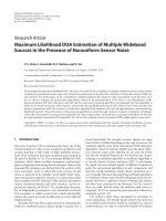
linear model works better than the affine model. The affine
model performs well when the exposure ratios are close; the
model becomes more and more insufficient as the exposure
ratios differ more. Figure 2 demonstrates this for a larger set
of exposure ratios, ranging from 2 to 50.
A superresolution algorithm requires an accurate mod-
eling of the imaging process. The restored image should b e
consistent with the observations given the imaging model.
A typical iterative SR algorithm (POCS-based [23], Bayesian
[24], iterated back-projection [25]) starts with an initial es-
timate, calculates an observation using the imaging model,
finds the residual between the calculated and real observa-
tions, and projects the residual back onto the initial estimate.
When the imaging model is not accurate or registration pa-
rameters are not estimated correctly, the algorithm would
fail. In this section, we conclude that nonlinear photomet-
ric models should be a part of SR algorithms when there is a
possibility of photometric diversity among input images.
3. SR UNDER PHOTOMETRIC DIVERSITY
When all input images are not photometrically identical,
there are two possible ways to enhance a reference image:

(i) spatial resolution enhancement and (ii) spatial resolution
and dynamic range enhancement. In (i), only spatial resolu-
tion of the reference image is improved. This requires pho-
tometric mapping of all input data to the reference image. In
(ii), both spatial resolution and dynamic range of the refer-
ence image are improved. This can be considered as a combi-
nation of high-dynamic-range imaging and superresolution
image restoration.
3.1. Spatial resolution enhancement
In spatial resolution enhancement, all input images are con-
verted to the tonal range of reference image. After photomet-
ric registration, a traditional SR reconstruction algorithm
can be applied. However, this is not a straightforward process
when the intensity mapping is nonlinear. Refer to Figure 3
that shows various intensity mapping functions (IMFs). Sup-
pose that z
1
is the reference image to be enhanced. Input im-
age z
2
is photometrically mapped onto z
1
in all cases. There
are four cases in Figure 3.
(i) In case (a), the input image z
2
has the same photo-
metric range with the reference image; so there is no
photometric registration necessary.
(ii) In case (b), the IMF is nonlinear; however, there is

no saturation. Therefore, the intensities of z
2
can be
mapped onto the range of z
1
using the IMF without
loss of information.
(iii) In case (c), there is bright saturation in z
2
. The IMF is
not a one-to-one mapping. The problematic region is
where the slope of the IMF is zero or close to zero. For
saturated regions, there is no information in z
2
corre-
sponding to z
1
. Therefore, perfect photometric map-
ping from z
2
to z
1
is not possible. When additive sen-
sor noise and quantization are considered, small-slope
(referring to the slope of the IMF) regions would also
be problematic in addition to the zero-slope (satura-
tion) regions. In these regions, noise and quantization
error in z
2
would be amplified when mapped onto z

1
,
and reconstruction would be affected negatively.
4 EURASIP Journal on Advances in Signal Processing
(a) (b) (c) (d)
(e) (f)
50
100
150
200
(g)
0
50
100
150
200
250
0 50 100 150 200 250
α
43
z
3
+ β
43
α
42
z
2
+ β
42

α
41
z
1
+ β
41
(h)
(i) (j)
50
100
150
200
(k)
0
50
100
150
200
250
0 50 100 150 200 250
g
43
(z
3
)
g
42
(z
2
)

g
41
(z
1
)
(l)
Figure 1: Comparison of affine and nonlinear photometric conversions. (a)–(d) are the images captured with different exposure rates. All
camera parameters other than the exposure rates are fixed. T he images are geomet rically registered. T he relative exposure rates are as follows:
(a) image z
1
with exposure rate 1/16; (b) image z
2
with exposure rate 1/4; (c) image z
3
with exposure rate 1/2; (d) image z
4
with exposure rate
1. Image z
4
is set as the reference image and other images are photometrically registered to it. The residuals and the registration parameters
are shown; (e) residual between z
4
and photometrically aligned z
1
using the affine model; (f) residual between z
4
and photometrically aligned
z
2
using the affine model; (g) residual between z

4
and photometrically aligned z
3
using the affine model; (h) the photometric mappings for
(e)–(g); (i) residual between z
4
and photometrically aligned z
1
using the nonlinear model; (j) residual between z
4
and photometrically
aligned z
2
using the nonlinear model; (k) residual between z
4
and photometrically aligned z
3
using the nonlinear model; (l) the photometric
mappings for (i)–(k).
(iv) In case (d), there are regions of small slope and large
slope. Large-slope regions are not an issue because
mapping from z
2
to z
1
would not create an y problem.
The problem is still with the small-slope regions (dark
saturation regions in z
2
), where quantization error and

noise are effective.
One solution to the saturation and noise amplification prob-
lems is to use a certainty function associated with each im-
age. The certainty function should weight the contribution
of each pixel in reconstruction based on the reliability of con-
version. If a pixel is saturated or close to saturation, then the
certainty function should be close to zero. If a pixel is from
a reliable region, then the certainty function should be close
to one. The issue of designing a certainty funct ion has been
investigated in HDR research. In [22], the certainty function
is defined according to the derivative of the CRF. The moti-
vation is that for pixels corresponding to low-slope regions
of the CRF, the reliability should also be low. In [13], the cer-
tainty function includes variances of the additive noise and
quantization errors in addition to the derivative of the CRF.
In [9], a fixed hat function is used. According to it, the mid-
range pixels have high reliability, while low-end and high-end
pixels have low reliability.
We now put these ideas in SR reconstruction. Let x be
the (unknown) high-resolution version of a reference image
z
r
,anddefineg
ri
(z
i
) as the IMF that takes z
i
and converts
it to the photometric range of z

r
(therefore, x ). Referring to
(5), g
ri
(z
i
) includes the CRF f (·), and gain α
ri
,andoffset β
ri
parameters:
g
ri

z
i

≡
f

α
ri
f
−1

z
i

+ β
ri


. (6)
We also need to model spatial transformations of the imag-
ing process. Define H
i
as the linear mapping that takes a
high-resolution image and produces a low-resolution image.
H
i
includes motion (of the camera or the objects in the
scene), blur (caused by the point spread function of the sen-
sor elements and the optical system), and downsampling.
(Details of H
i
modeling can be found in the special issue of
M. Gevrekci and B. K. Gunturk 5
0
5
10
15
20
25
30
35
40
Error
0 5 10 15 20 25 30 35 40 45 50
Exposure ratios
Affine error
Nonlinear error

Figure 2: Root-mean-square error (RMSE) values of photometri-
cally registered images with relative exposure rates of 2, 4, 8, 16, 32,
50. The RMSE values (green points) for affine mappings are 14.8,
21.1, 27.8, 34.3, 38.7, 40.7. The RMSE values (blue points) for non-
linear mappings are 11.2, 11.6, 11.4, 13.5, 15.9, 17.2.
the IEEE Signal Processing Magazine [3] and the references
therein.)
When H
i
is applied on x, it should produce the photo-
metrically converted ith observation, g
ri
(z
i
). That is, we need
to find x that produces g
ri
(z
i
) when H
i
is applied to it, for all
i. The least-squares solution to this problem would minimize
the following cost function:
C(x)
=

i



g
ri

z
i

−
H
i
x


2
. (7)
As explained earlier, the problem associated with the satu-
ration of the IMF can be solved using a certainty funct ion,
w(z
i
). We formulate our equations using a generic function
w(z
i
). Our specific choice will be given in the experimental
results Section 5. We now define a diagonal matrix W
i
whose
diagonal is w(z
i
), and incorpora te this matrix into (7)tofind
the weig hted least-squares solution. The new cost function is
C(x)

=
1
2

i

g
ri

z
i

− H
i
x

T
W
i

g
ri

z
i

− H
i
x


. (8)
Since dimensions of the matrices are large, we want to avoid
matrix inversion and apply the gradient descent technique to
find x that minimizes this cost function. Starting with an ini-
tial estimate x
(0)
, each iteration updates x
(0)
in the direction
of the negative gradient of C(x):
x
(k+1)
= x
(k)
+ γ

i
H
T
i
W
i

g
ri

z
i

−

H
i
x
(k)

,(9)
where γ is the step size at the kth iteration. Defining Φ as
the negative gradient of C(x), the exact line search that min-
imizes C(x
(k)
+ γΦ) y ields the step size:
γ
=
Φ
T
Φ
Φ
T


i
H
T
i
W
i
H
i

Φ

, (10)
with
Φ
=

i
H
T
i
W
i

g
ri

z
i

−
H
i
x
(k)

. (11)
An iteration of the algorithm is illustrated in Figure 4,and
the pseudocode is given in Algorithm 1. Note that in imple-
mentation, it is not necessary to construct matrices or vectors
to follow the steps of the algorithm. Application of H
i

can b e
implemented as warping an image geometrically, convolving
with the point spread function (PSF), and downsampling.
Similarly, H
T
i
can be implemented as upsampling with zero
insertion, convolving with a flipped PSF, and back-warping
[13]. The step size γ can be obtained using the same princi-
ples.
3.2. Spatial resolution and dynamic range
enhancement
Here, the goal is to produce a high-resolution and high-
dynamic range image. One option is to obtain the high-
resolution version of each input image using the algorithm
given in Algorithm 1, and then apply HDR image construc-
tion to these high-resolution images.
A second option is to derive the high-resolution irra-
diance q directly. This requires formulating the image ac-
quisition f rom the unknown high-resolution irradiance q to
each observation z
i
. Adding the spatial processes (geometric
warping, blurring with the PSF, and downsampling) to (4),
the imaging process can be formulated as
z
i
= f

a

i
H
i
q + b
i

, (12)
where H
i
is the linear mapping (including warping, blur-
ring, and downsampling operations) from a high-spatial-
resolution irradiance signal to a low-spatial-resolution irra-
diance signal. f (
·), a
i
,andb
i
are the CRF, gain, and offset
terms as in (4).
This time, the weighted least-squares estimate of q mini-
mizes the following cost function:
C(q)
=
1
2

i

f
−1


z
i

− b
i
a
i
−H
i
q

T
W
i

f
−1

z
i

− b
i
a
i
−H
i
q


.
(13)
This cost function is basically analogous to the cost function
in (8). Starting with an initial estimate for q, the rest of al-
gorithms work similar to the one in Algorithm 1.Theonly
difference is that intensity-to-intensity mapping g
ri
(·)in(8)
is replaced w ith intensity-to-irradiance mapping ( f
−1
(·) −
b
i
)/a
i
. Unlike the intensity-to-intensity mapping, intensity-
to-irradiance mapping requires explicit estimation of the
CRF, gain, and offset parameters.
6 EURASIP Journal on Advances in Signal Processing
z
2
z
1
(a)
z
2
z
1
(b)
z

2
z
1
(c)
z
2
z
1
(d)
z
2
z
2
z
2
z
2
z
1
z
1
z
1
z
1
(e)
Figure 3: Various photometric conversion scenarios. First row illustrates possible photometric conversion functions. Second and third rows
show example images with such photometric conversion.
H
T

1
H
1
H
2
.
.
.
H
N
H
T
2
H
T
N
x
(k+1)
g
r1
(z
1
) w(z
1
)
w(z
N
)
w(z
2

)g
r2
(z
2
)
g
rN
(z
N
)
x
(k)
γ
Figure 4: Spatial resolution enhancement framework using IMF.
g
ri
(·) is the IMF that converts input image z
i
to the photometric
range of reference image. H
i
applies spatial transformations, con-
sisting of geometric warping, blurring, and downsampling. Sim-
ilarly, H
i
T
applies upsampling with zero insertion, blurring, and
back-warping. γ is the step size of the update; it is computed at each
iteration.
We write the iterative step to estimate q as follows:

q
(k+1)
= q
(k)
+ γ

i
H
T
i
W
i

f
−1

z
i

−
b
i
a
i
− H
i
q
(k)

, (14)

where γ is the step size. It is obtained similar to the one in (9).
The details of this approach are trivial given the derivations
in the previous section; therefore, we leave it to the reader.
In [ 13], we also investigated this joint spatial and dy-
namic range enhancement idea. The approach in [13]issim-
ilar to the one (irradiance-domain solution) given in this
section. As we mentioned in Section 1,in[13], we applied
Taylor series expansion to the inverse of the CRF to end up
with a specific certainty function. The algorithm requires es-
timation of the CRF and the variances of noise and quanti-
zation error. It also includes a spatial regularization term in
the reconstruction. We refer the readers to [13] for details.
Thederivationinthissectioncanbeconsideredasagen-
eralizationofthesolutiongivenin[13]; here, the certainty
function is not specified. In practice, the method in [ 13]and
the irradiance-domain solution of this section work similarly
with the proper selection of certainty functions.
Note that this approach estimates the irradiance q,which
needs to be compressed in dynamic range to display on lim-
ited dynamic range displays. Displaying HDR images on lim-
ited dynamic-ra nge displays is an active research area [26].
3.3. Certaint y function
As we have discussed in Section 3.1, the information com-
ing from low-end and high-end of the intensity range is n ot
reliable due to noise, quantization, and saturation. If used,
these unreliable pixels would degrade the restoration. In [9],
a generalized hat function is proposed to reduce the effect of
unreliable pixels. We use a piecewise linear certainty func-
tion in our experiments. The certainty function is shown in
Figure 5. The intensity breakpoints in the certainty function

are 15 and 240, and they were determined by trial and error.
Figure 6 shows an example to demonstrate the reliability
of pixels and the effect of the certainty function. The first row
in the figure shows photometric conversion from an over-
exposed image to an underexposed image. This is the sce-
nario in Figure 3(c). Figure 6(a) is the reference image, and
Figure 6(b) is the geometrically warped input image which
M. Gevrekci and B. K. Gunturk 7
(1) Requirements:
• Set or estimate the point spread function (PSF) of the camer a: h
• Set the resolution enhancement factor: F
• Set the number of iterations: K
(2) Initialization:
• Choose the reference image z
r
• Interpolate z
r
by the enhancement factor F to obtain x
(0)
(3) Parameter estimation:
• Estimate the spatial registration parameters between z
r
and z
i
, i = 1, , N
• Estimate the IMFs, g
ri
(z
i
), between z

r
and z
i
, i = 1, , N
(4) Iterations:
• For k = 0toK − 1
• Create a zero-filled initial image Ψ with the same size as x
(0)
• For i = 1toN
• Find H
i
x
(k)
with the following steps:
• Convolv e x
(k)
with the PSF h
• Warp and downsample the convolved image onto
the input z
i
• Find the residual g
ri
(z
i
) − H
i
x
(k)
• Find the weight image w(z
i

) and multiply it pixel by pixel
with the residual g
ri
(z
i
) − H
i
x
(k)
• Obtain H
T
i
W
i
g
ri
(z
i
) − H
i
x
(k)
with the following steps:
• Upsample the weighted residual by the factor F with
zero insertion
• Convolve the result with the flipped PSF h
• Warp the result to the coordinates of x
(k)
• Update Ψ: Ψ ← Ψ + H
T

i
W
i
(g
ri
(z
i
) − H
i
x
(k)
)
• Calculate γ
• Update the current estimate: x
(k+1)
= x
(k)
+ γΨ
Algorithm 1: Pseudocode of the spatial enhancement algorithm.
0
0.2
0.4
0.6
0.8
1
Weights
0 50 100 150 200 250
Input image intensity range
Figure 5: Piecewise linear certainty function used in the experi-
ments. The intensity breakpoints in the figure are 15 and 240.

we want to map onto the reference image tonally. Figure 6(c)
shows the residual between the input and the reference im-
ages without photometric registration. Figure 6(d) shows the
residual after the application of IMF to the input image.
Clearly, saturated pixels are not handled well: residuals for
these pixels are large. The weights for each pixel in the im-
age are calculated with application of the certaint y function
on the input image; they are shown in Figure 6(e). Examin-
ing Figures 6(d) and 6(e), it can be seen that the weights for
unreliable saturated pixels are low, as expected. Figure 6(f)
shows the final residual after the application of the weight
image (Figure 6(e)) on the residual image (Figure 6(d)).
The second row in Figure 6 shows an example of tonal
conversion from an underexposed image to an overexposed
image. This is the scenario in Figure 3(d). Figure 6(g) is the
reference image and Figure 6(h) is the geometrically warped
input image. Here, photometric transformation can be per-
formed without any problem for high-end of intensity range.
The problem is the low-end, dark saturation regions in the
input image. Figure 6(j) shows the residual after tonal con-
version. Figure 6(k) is the certainty image. As seen, the un-
reliable dark saturation regions are having low weights. Fig-
ure 6(l) shows the weighted residual obtained by multiplying
the residual image with the corresponding certainty image.
In the weighted residual image, large residual values (that
would degrade SR reconstruction) are eliminated or reduced
significantly.
8 EURASIP Journal on Advances in Signal Processing
(a) (b) (c) (d) (e) (f)
(g) (h) (i) (j) (k) (l)

Figure 6: Weighting function effect on residuals. First row performs conversion onto low-exposure reference while second row has a ref-
erence with high exposure: (a) reference image; (b) geometrically warped input image; (c) residual image without tonal conversion; (d)
residual image using nonlinear tonal conversion; (e) certainty image using hat function as weighting and image (b) as input; (f) weighted
residual obtained multiplying residual image in (d) by certainty image in (e); (g) reference image; (h) geometrically warped input image;
(i) residual image without tonal conversion; (j) residual image using nonlinear tonal conversion; (k) certainty image using hat function as
weighting and image (g) as input; (l) weighted residual obtained multiplying residual image i n (j) by certainty image in (k).
(a) (b) (c)
(d) (e)
Figure 7: Five images of “Facility I” data set that includes 22 images are displayed here. Exposure durations of (a)–(e) are 1/25, 1/50, 1/100,
1/200, and 1/400 seconds, respectively.
4. GEOMETRIC AND PHOTOMETRIC REGISTRATIONS
SR requires accurate geometric and photometric registra-
tions. If the actual CRF and the exposure r a tes are unknown,
the images must be geometrically registered before these pa-
rameters can be estimated. On the other hand, geometric
registration is problematic when images are not photomet-
rically registered. There are three possible approaches to this
problem.
(A1) Images are first geometrically registered using an algo-
rithm that is insensitive to photometric changes. This
is followed by photometric registration.
(A2) Images are first photometrically registered using an
algorithm that is insensitive to geometric misalign-
ments. This is followed by geometric registration.
(A3) Geometric and photometric registration parameters
are estimated jointly.
M. Gevrekci and B. K. Gunturk 9
(a) (b) (c)
(d) (e) (f)
Figure 8: Six images of “Facility II” data set that includes 31 images are displayed here. Exposure durations of (a)–(f) are 1/25, 1/50, 1/100,

1/200, 1/400, and 1/800 seconds, respectively.
(a) (b) (c) (d)
(e) (f) (g) (h)
Figure 9: Cropped regions of observation and SR results: (a)–(e) input images; (f) SR when (a) is the reference image; (g) SR when (e) is
the reference image; (h) SR using the technique presented in Section 3.2.
There are few algorithms that can be utilized for these ap-
proaches. In [27], an exposure-insensitive motion estima-
tion algorithm based on the Lucas-Kanade technique is pro-
posed to estimate motion vectors at each pixel. Although this
method can be used to estimate large and dense motion field,
it has the downside that it requires preknowledge of the CRF.
Another exposure-insensitive algorithm is proposed in [28].
It is based on bitmatching on binary images. Although it does
not require knowing CRF in advance, the algorithm is lim-
ited to global translational motion. In [17], an IMF estima-
tion algorithm that does not require geometric registration
is proposed. It is based on the idea that histogram specifica-
tion gives the intensity mapping between two images when
there is no saturation or significant geometric misalignment.
And finally in [29], a joint geometric and photometric reg-
istration algorithm is proposed. There, the problem is for-
mulated as a global parameter estimation, where the param-
eters jointly represent geometric transformation, exposure
rate, and CRF. Two potential problems associated with this
approach are (1) getting stuck at a local minimum and (2)
limitation of using parametric CRF.
We take approach (A1) in our experiments. This is also
the approach in [13]. References [5, 12] take the same ap-
proach except for the photometric model. For geometric reg-
istration, we use a feature-based algorithm, which requires

robust exposure-insensitive feature extraction and matching.
10 EURASIP Journal on Advances in Signal Processing
(a) (b) (c) (d)
(e) (f) (g)
Figure 10: Cropped regions of observation and SR results: (a)–(d) input images; (e) SR when (d) is the reference image; (f) SR when (a) is
the reference image; (g) SR using the technique presented in Section 3.2.
(a) (b)
Figure 11: Comparison of weighting function during spatial resolution enhancement. The lowest exposed image is chosen as reference. (a)
SR reconstruction using identity weight, (b) SR reconstruction using a hat function as weight.
In our experiments, feature points are first extracted using
the Harris corner detector [30]. Although the Harris corner
detector is not invariant to illumination changes in general,
it worked well in our experiments. These feature points are
matched using nor malized cross-correlation, which is insen-
sitive to contrast changes. The RANSAC method [31] is then
used to eliminate the outliers and estimate the homogra-
phies. After geometric registration comes photometric reg-
istration. There are various methods available in the litera-
ture to estimate IMF and CRF as we discussed earlier. In our
experiments, we use [19]toestimateIMF,CRF,andtheex-
posure rate.
5. EXPERIMENTS AND RESULTS
We conducted experiments to demonstrate the proposed
SR algorithms. (A Matlab toolbox can be downloaded from
[32].) We captured two data sets with a handheld digital cam-
era. These data sets are shown in Figures 7 and 8. The reso-
lution enhancement factor is four and the number of itera-
tions was set to two in all experiments. The PSF is taken as
a Gaussian window of size [7
× 7] and of variance 1.7. The

results are shown in Figures 9 and 10. For the spatial-only en-
hancement approach, we did experiments when the reference
is chosen as an overexposed image and also when it is chosen
M. Gevrekci and B. K. Gunturk 11
as an underexposed image to show the robustness of the algo-
rithm. For the irradiance-domain spatial and dynamic range
enhancement approaches, we created an initial estimate by
applying a standard HDR image construction algorithm [9].
The initial estimate is then updated iteratively.
For comparison purposes, we provided cropped regions
of results and transformed input images in Figure 9.Fig-
ures 9(a), 9(b), 9(c), 9(d), 9(e) are the bilinearly interpo-
lated observations with different exposure rates chosen from
the 22 input images. Each observation contains a different
portion of the existing tonal range. Figure 9(f) is the SR
result obtained when the overexposed image, (Figure 9(a)),
is chosen as the reference image. Comparison of Figures
9(a) and 9(f) shows the improvement i n resolution. Simi-
larly, Figure 9(g) is obtained when the underexposed image,
(Figure 9(e)), is set as the reference image. The resolution en-
hancement is again clear. Figure 9(h) is the result of the res-
olution and dynamic-range enhancement algorithm. Notice
that both spatial resolution and dynamic range are improved.
(Note that the result of an HDR algorithm would have higher
dynamic range than a standard display or printing device.
Therefore, an HDR image should be compressed in range to
output in such LDR devices. There are complex display algo-
rithms [26]. In this paper, we used a simple gamma correc-
tion to display the result. The gamma correction parameter
is 0.5.) Figure 10 shows the results for the second data set.

The discussion is parallel to the discussion of first data set,
therefore, it is excluded for conciseness.
Finally, we wanted to test the effect of the weighting func-
tion in SR reconstruction. Figures 11(a) and 11(b) aim to in-
crease both spatial resolution and dynamic range, and dif-
fer only in their weighting function. Figure 11(a) shows SR
result using a unity weight. Notice the loss of information
in details and color. Color artifacts occur in this case as the
saturated pixels are not handled properly. Strips on the ware-
house can hardly be observed and the sky color is washed out
due to fusion with saturated residuals. There is also contour-
ing ar tifact. Figure 11(b) shows the result using the proposed
hat function for weighting. Texture and colors are preserved
compared to Figure 11(a).
6. CONCLUSIONS
In this paper, we showed how to do SR when the photo-
metric characteristics of the input images are not identical.
We showed two possible approaches, one of them enhanc-
ing spatial resolution only, and the other enhancing spa-
tial resolution and dynamic range jointly. We demonstrated
that nonlinear photometric modeling should be preferred to
affine photometric modeling. We also discussed that an ap-
propriate weighting function is necessary to handle satura-
tion. O ther SR reconstruction techniques can be modified
and applied as long as an appropriate photometric registra-
tion is included.
Although geometric registration is a complicated task
for differently exposed images, we achie ved a success using
feature-based registration without the need of CRF. A se-
quential approach is useful: similarly exposed images would

produce similar features; therefore, correct geometric regis-
tration would be easier to estimate among similarly exposed
images compared to images with large exposure differences.
Therefore, one may find the homographies among similarly
exposed images, and then combine the homographies to find
the homography between any two images. In our experi-
ments, we chose a reference image from the middle of the
tonal range. Homographies of input images are found with
respect to this reference image. The homography between
any two of the input images can then be found by multiplying
the corresponding homography matrices. Photometric regis-
tration is trivial after the geometric registration.
In this paper, we considered static scenes only. Estimation
of motion parameters for nonstatic scenes is left as a future
work. Also, we only considered global photometric changes.
In experiments, we only considered the exposure rate change
which acts globally on image. In general, a dense photomet-
ric model is necessary to handle local photometric changes.
That is, accurate geometric and photometric registrations of
photometrically different image certainly require further re-
search.
ACKNOWLEDGMENT
This work was supported by the National Science Founda-
tion under Grant no. ECS-0528785.
REFERENCES
[1] MotionDSP, April 2007, />[2] QELabs, April 2007, />[3] S. C. Park, M. K. Park, and M. G. Kang, “Super-resolution im-
age reconstruction: a technical overview,” IEEE Signal Process-
ing Magazine, vol. 20, no. 3, pp. 21–36, 2003.
[4] S. Chaudhuri, Ed., Super-Resolution Imaging, Springer, Berlin,
Germany, 2001.

[5] D. Capel, Image Mosaicing and Super-Resolution, Springer,
Berlin, Germany, 2004.
[6] S. Farsiu, D. Robinson, M. Elad, and P. Milanfar, “Advances
and challanges in super-resolution,” International Journal of
Imaging Systems and Technology, vol. 14, no. 2, pp. 47–57,
2004.
[7] S. Borman and R. L. Stevenson, “Super-resolution from image
sequences: a review,” in Proceedings of the Midwest Symposium
on Circuits and Systems, vol. 5, pp. 374–378, Notre Dame, Ind,
USA, April 1998.
[8] E. Reinhard, G. Ward, S. Pattanaik, and P. Debevec, High Dy-
namic Range Imaging: Acquisition, Display, and Image-Based
Lighting, Morgan Kaufmann, San Francisco, Calif, USA, 2006.
[9] P. E. Debevec and J. Malik, “Recovering high dynamic range
radiance maps from photographs,” in Proceedings of the 24th
Annual Conference on Computer Graphics and Interactive Tech-
niques (SIGGRAPH ’97), pp. 369–378, Los Angeles, Calif, USA,
August 1997.
[10] S. Mann and R. W. Picard, “Being ‘undigital’ with digital cam-
eras: extending dynamic range by combining differently ex-
posed pictures,” in Proceedings of the 48th IS&T’s Annual Con-
ference, pp. 442–448, Washington, DC, USA, May 1995.
[11] M. A. Robertson, S. Borman, and R. L. Stevenson, “Dynamic
range improvement through multiple exposures,” in Proceed-
ings of IEEE International Conference on Image Processing (ICIP
’99), vol. 3, pp. 159–163, Kobe, Japan, October 1999.
12 EURASIP Journal on Advances in Signal Processing
[12] D. Capel and A. Zisserman, “Computer vision applied to super
resolution,” IEEE Signal Processing Magazine,vol.20,no.3,pp.
75–86, 2003.

[13] B. K. Gunturk and M. Gevrekci, “High-resolution image re-
construction from multiple differently exposed images,” Signal
Processing Letters, vol. 13, no. 4, pp. 197–200, 2006.
[14] A. Litvinov and Y. Y. Schechner, “Radiomet ric framework for
image mosaicking,” Journal of the Optical Society of America A,
vol. 22, no. 5, pp. 839–848, 2005.
[15] D. Hasler and S. S
¨
usstrunk, “Mapping colour in image stitch-
ing applications,” Journal of Visual Communication and Image
Representation, vol. 15, no. 1, pp. 65–90, 2004.
[16] S. K. Nayar, K. Ikeuchi, and T. Kanade, “Shape from inter-
reflections,” International Journal of Computer Vision, vol. 6,
no. 3, pp. 173–195, 1991.
[17] M. D. Grossberg and S. K. Nayar, “Determining the camera
response from images: what is knowable?” IEEE Transactions
on Pattern Analysis and Machine Intelligence, vol. 25, no. 11,
pp. 1455–1467, 2003.
[18] S. Mann, C. Manders, and J. Fung, “Painting with looks: pho-
tographic images from video using quantimetric processing,”
in Proceedings of the 10th ACM International Conference on
Multimedia (MULTIMEDIA ’02), pp. 117–126, Juan les Pins,
France, December 2002.
[19] S. Mann and R. Mann, “Quantigraphic imaging: estimating
the camera response and exposures from differently exposed
images,” in Proceedings of IEEE Computer Society Conference
on Computer Vision and Pattern Recognition (CVPR ’01), vol. 1,
pp. 842–849, Kauai, Hawaii, USA, December 2001.
[20] T. Mitsunaga and S. K. Nayar, “Radiometric self calibration,”
in Proceedings of IEEE Computer Society Conference on Com-

puter Vision and Pattern Recognition (CVPR ’99), vol. 1, pp.
374–380, Fort Collins, Colo, USA, June 1999.
[21] Y. Tsin, V. Ramesh, and T. Kanade, “Statistical calibration of
CCD imaging process,” in Proceedings of the 8th IEEE Interna-
tional Conference on Computer Vision (ICCV ’01), vol. 1, pp.
480–487, Vancouver, BC, Canada, July 2001.
[22] S. Mann, “Comparametric equations with practical applica-
tions in quantigraphic image processing,” IEEE Transactions
on Image Processing, vol. 9, no. 8, pp. 1389–1406, 2000.
[23] A. J. Patti, M. I. Sezan, and A. M. Tekalp, “Superresolu-
tion video reconstruction with arbitrary sampling lattices and
nonzero aperture time,” IEEE Transactions on Image Process-
ing, vol. 6, no. 8, pp. 1064–1076, 1997.
[24] R. R. Schultz and R. L. Stevenson, “Extraction of high-
resolution frames from video sequences,” IEEE Transactions on
Image Processing, vol. 5, no. 6, pp. 996–1011, 1996.
[25] M. Irani and S. Peleg, “Improving resolution by image regis-
tration,” CVGIP: Graphical Models & Image Processing, vol. 53,
no. 3, pp. 231–239, 1991.
[26] R. Fattal, D. Lischinski, and M. Werman, “Gradient do-
main high dynamic range compression,” ACM Transactions on
Graphics, vol. 21, no. 3, pp. 249–256, 2002.
[27] S. B. Kang, M. Uyttendaele, S. Winder, and R. Szeliski, “High
dynamic range video,” ACM Transactions on Graphics, vol. 22,
no. 3, pp. 319–325, 2003.
[28] G. Ward, “Fast, robust image registration for compositing high
dynamic range photographs from hand-held exposures,” Jour-
nal of Graphics Tools, vol. 8, no. 2, pp. 17–30, 2003.
[29] F. M. Candocia, “Jointly registering images in domain and
range by piecewise linear comparametric analysis,”

IEEE
Transactions on Image Processing, vol. 12, no. 4, pp. 409–419,
2003.
[30] C. G. Harris and M. Stephens, “A combined corner and edge
detector,” in Proceedings of the 4th Alvey Vision Conference,pp.
147–151, Manchester, UK, August-September 1988.
[31] M. A. Fischler and R. C. Bolles, “Random sample consensus: a
paradigm for model fitting with applications to image analy-
sis and automated cartography,” Communications of the ACM,
vol. 24, no. 6, pp. 381–395, 1981.
[32] M. Gevrekci and B. K. Gunturk, “Matlab user interface
for super resolution image reconstruction for illumina-
tion varying and Bayer pattern images,” April 2007,
/>Murat Gevrekci received his B.S. degree in
electrical engineering from Bilkent Univer-
sity, Ankara, Turkey, in 2004, and the M.S.
degree in electrical and computer engineer-
ing from Louisiana State University, Baton
Rouge, La, in 2006. He is currently pursu-
ing his Ph.D. degree at Louisiana State Uni-
versity. His research interests include im-
age/video processing, parallel image pro-
cessing, and computer vision. He published
several peer-reviewed articles and served as a Technical Reviewer
for various journals in the field of signal processing. He is a Stu-
dent Member of the IEEE.
Bahadir K. Gunturk received his B.S. de-
gree in electrical engineering from Bilkent
University, Ankara, Turkey, in 1999, and
M.S. and Ph.D. degrees in electrical engi-

neering from Georgia Institute of Technol-
ogy, Atlanta, Ga, in 2001 and 2003, respec-
tively. He is currently an Assistant Professor
at Louisiana State University, Baton Rouge,
La. His main research interest is computer
vision. He is a Member of the IEEE.