Báo cáo hóa học: " Research Article Calculation Scheme Based on a Weighted Primitive: Application to Image Processing Transforms" docx

Hindawi Publishing Corporation
EURASIP Journal on Advances in Signal Processing
Volume 2007, Article ID 45321, 17 pages
doi:10.1155/2007/45321
Research Article
Calculation Scheme Based on a Weighted Primitive:
Application to Image Processing Transforms
Mar
´
ıa Teresa Signes Pont, Juan Manuel Garc
´
ıa Chamizo, Higinio Mora Mora,
and Gregorio de Miguel Casado
Depar t amento de Tecnolog
´
ıa Inform
´
atica y Computaci
´
on, Universidad de Alicante, 03690 San Vicente del Raspeig,
03071 Alicante, Spain
Received 29 September 2006; Accepted 6 March 2007
Recommended by Nicola Mastronardi
This paper presents a method to improve the calculation of functions which specially demand a great amount of computing
resources. The method is based on the choice of a weighted primitive which enables the calculation of function values under
the scope of a recursive operation. When tackling the design level, the method shows suitable for developing a processor which
achieves a satisfying trade-off between time delay, area costs, and stability. The method is particularly suitable for the mathe-
matical transforms used in signal processing applications. A generic calculation scheme is developed for the discrete fast Fourier
transform (DFT) and then applied to other integral transforms such as the discrete Hartle y transform (DHT), the discrete co-
sine transform (DCT), and the discrete sine transform (DST). Some comparisons with other well-known proposals are also
provided.

Copyright © 2007 Mar
´
ıa Teresa Signes Pont et al. This is an open access article distributed under the Creative Commons
Attribution License, which permits unrestricted use, distribution, and reproduction in any medium, provided the original work is
properly cited.
1. INTRODUCTION
Mathematical notation aside, the motivation behind inte-
gral transforms is easy to understand. There are many classes
of problems that are extremely difficult to solve or, at least,
quite unwieldy from the algebraic standpoint in their origi-
nal domains. An integra l transform maps an equation from
its original domain (time or space domain) into another
domain (frequency domain). Manipulating and solving the
equation in the target domain is, ideally, easier than ma-
nipulating and solving it in the original domain. The solu-
tion is then mapped back into the original domain. Integral
transforms work because they are based upon the concept of
spectral factorization over orthonormal bases. Equation (1)
shows the generic formulation of a discrete integral trans-
form where f (x), 0
≤ x<N,andF(u), 0 ≤ u<N, are the
original and the transformed sequences, respectively. Both
have N
= 2
n
values, n ∈ N and T(x, u) is the kernel of
the transform
F(u)
=
N−1


x=0
T(x, u) f (x). (1)
The inverse transform can be defined in a similar way.
Table 1 shows some integral transforms (j
=
√
−1asusual).
The Fourier transform (FT) is a reference tool in image
filtering [1, 2] and reconstruction [3]. A fast Fourier trans-
form (FFT) scheme has been used in OFDM modulation (or-
thogonal frequency division multiplexing) and has shown to
be a valuable tool in the scope of communications [4, 5]. The
most relevant algorithm for FFT calculation was developed
in 1965 by Cooley and Tukey [6]. It is based on a succes-
sive folding scheme and its main contribution is a compu-
tational complexity reduction that decreases from O(N
2
)to
O(N
· log
2
N). The variants of FFT algorithms follow differ-
ent ways to perform the calculations and to store the inter-
vening results [7]. These differences give rise to different im-
provements such as memory saving in the case of in-place al-
gorithms, high speed for self-sorting algorithms [8] or regu-
lar architectures in the case of constant geometry algorithms
[9]. These improvements can be extended if combinations of
the different schemes are envisaged [10]. The features of the

different algorithms point to different hardware trends. The
in-place algorithms are generally implemented by pipelined
architectures that minimize the latency between stages and
the memory [11] whereas the constant geometry algorithms
2 EURASIP Journal on Advances in Signal Processing
Table 1: Some integral transforms.
Transform Kernel T(x, u) Remarks
Fourier
1
N
exp

−
2 jπux
N

Trigonometric kernel
Hartley cos

2πux
N

+sin

2πux
N

Trigonometric kernel
Cosine
e(k)cos

(2x +1)πu
2N
Trigonometric kernel
with e(0)
=
1
√
2
,
e(k)
= 1, 0 <k<N
Sine
e(k)sin
(2x +1)πu
2N
Trigonometric kernel
with e(0)
=
1
√
2
,
e(k)
= 1, 0 <k<N
have an easier control because of their regular structure based
on a constant indexation through all the stages. This allows
parallel data processing by a column of processors with a
fixed interconnecting net [12, 13].
The Hartley transform is a Fourier-related transform
which was introduced in 1942 by Hartley [14] and is very

similar to the discrete Fourier transform (DFT), w ith analo-
gous applications in signal processing and related fields. Its
main distinction from the DFT is that it transforms real in-
puts into real outputs, with no intrinsic involvement of com-
plex numbers. The discrete Hartley transform (DHT) ana-
logue of the Cooley-Tukey algorithm is commonly known as
the fast Hartley transform (FHT) algorithm, and was first de-
scribed in 1984 by Bracewell [15–17]. The transform can be
interpreted as the multiplication of the vector (x
0
, , x
N−1
)
by an N
×N matrix; therefore, the discrete Hartley transform
is a linear operator. The matrix is invertible and the DHT is
its own inverse up to an overall scale factor. This FHT al-
gorithm, at least when applied to power-of-two sizes N,is
the subject of a patent issued in 1987 to the University of
Stanford. The University of Stanford placed this patent in the
public domain in 1994 [18]. The DHT algorithms are typi-
cally slightly less efficient (in terms of the number of floating-
point operations) than the corresponding FFT specialized for
real inputs or outputs [19, 20]. The latter authors published
the algorithm which achieves the lowest operation count for
the DHT of power-of-two sizes by employing a split-radix al-
gorithm, similar to that of the FFT. This scheme splits a DHT
of length N into a DHT of length N/2 and two real-input
DFTs (not DHTs) of length N/4. A priori, since the FHT and
the real-input FFT algorithms have similar computational

structures, none of them appears to have a substantial speed
advantage [21]. As a practical matter, highly optimized real-
input FFT libraries are available from many sources whereas
highly optimized DHT libraries are less common. On the
other hand, the redundant computations in FFTs due to real
inputs are much more difficult to eliminate for large prime
N, despite the existence of O(N
· log
2
N)complex-dataal-
gorithms for that cases. This is because the redundancies are
hidden behind intricate permutations and/or phase rotations
in those algorithms. In contrast, a standard prime-size FFT
algorithm such as Rader’s algorithm can be directly applied
to the DHT of real data for roughly a factor of two less com-
putation than that of the equivalent complex FFT. This DHT
approach currently appears to be the only way known to ob-
tain such factor-of-two savings for large prime-size FFTs of
real data [22]. A detailed analysis of the computational cost
and specially of the numerical stability constants for DHT
of types I–IV and the related matr ix algebras is presented by
Arico et al. [23]. The authors prove that any of these DHTs of
length N
= 2
t
can b e factorized by means of a divide–and–
conquer strategy into a product of sparse, orthogonal matri-
ces where in this context sparse means at most two nonzero
entries per row a nd column. The sparsity joint with orthog-
onality of the matrix factors is the key for proving that these

new algorithms have low arithmetic costs and an excellent
normwise numerical stability.
DCT is often used in signal and image processing, es-
pecially for lossy data compression, because it has a strong
“energy compaction” property: most of the signal informa-
tion tends to be concentrated in a few low-frequency com-
ponents of the DCT [24, 25]. For example, the DCT is used
in JPEG image compression, MJPEG, MPEG [ 26], and DV
video compression. The DCT is also widely employed in solv-
ing partial differential equations by spectral methods [27]
and fast DCT algorithms are used in Chebyshev approxima-
tion of arbitrary functions by series of Chebyshev polynomi-
als [28]. Although the direct application of these formulas
would require O(N
2
) operations, it is possible to compute
them with a complexity of only O(N
· log
2
N)byfactoriz-
ing the computation in the same way as in the fast Fourier
transform (FFT). One can also compute DCTs via FFTs com-
bined with O(N) pre- and post-processing steps. In princi-
ple, the most efficient algorithms are usually those that a re
directly specialized for the DCT [29, 30]. For example, par-
ticular DCT algorithms resemble to have a widespread use
for transforms of small, fixed sizes such as the 8
×8DCTused
in JPEG compression, or the small DCTs (or MDCTs) typi-
cally used in audio compression. Reduced code size may also

be a reason for using a specialized DCT for embedded-device
applications. However, e ven specialized DCT algorithms are
typically closely related to FFT algorithms [22]. Therefore,
any improvement in algorithms for one transform will the-
oretically lead to immediate gains for the other transforms
too [31]. On the other hand, highly optimized FFT programs
are widely available. Thus, in practice it is often easier to ob-
tain high performance for generalized lengths of N with FFT-
based algorithms. Performance on modern hardware is typ-
ically not simply dominated by arithmetic counts and opti-
mization requires substantial engineering effort.
As DCT which is equivalent to a DFT of real and even
functions, the discrete sine transform (DST) is a Fourier-
related transform using a purely real matrix [25]. It is equiv-
alent to the imaginary parts of a DFT of roughly twice
the length, operating on real data with odd symmetry. As
forDCT,fourmaintypesofDSTcanbepresented.The
boundary conditions relate the various DCT and DST types.
Mar
´
ıa Teresa Signes Pont et al. 3
Table 2: Definition of the operation ⊕ for k = 1.
a ⊕b 01 = 110= 00 = 011=−1
01 = 1 α + βα α− β
10
= 00 = 0 β 0 −β
11
=−1 −α + β −α −α −β
The applications of DST are similar to those for DCT as well
as its computational complexity. The problem of reflecting

boundary conditions (BCs) for blurring models that lead to
fast algorithms for both deblurring and detecting the regu-
larization parameters in the presence of noise is improved by
Serra-Capizzano in a recent work [32]. The key point is that
Neumann BC matrices can be simultaneously diagonalized
by the fast cosine transform DCT III and Serra-Capizzano
introduces antireflective BCs that can be related to the al-
gebra of the matrices that can be simultaneously diagonal-
ized by the fast sine transform DST I. He shows that, in the
generic case, this is a more natural modeling whose features
are both, on one hand a reduced analytical error, since the
zero (Dirichlet) BCs lead to discontinuity at the boundaries,
the reflecting (Neumann) BCs lead to C
◦
continuity at the
boundaries, while his proposal leads to C
1
continuity at the
boundaries, and on the other hand fast numerical algorithms
in real arithmetic for deblurring and estimating regulariza-
tion parameters.
This paper presents a method that performs function
evaluation by means of successive iterations on a recursive
formula. This formula is a weighted sum of two operands
and it can be considered as a primitive operation just as com-
putational usual primitives such as addition and shift. The
generic definition of the new primitive can be achieved by a
two-dimensional table in which the cells store combinations
of the weighting parameters. This evaluation method is suit-
able for a great a mount of functions, particularly when the

evaluation needs a lot of computing resources, and allows
implementation schemes that offer a good balance between
speed, area saving, and error containing. This paper is fo-
cused on the application of the method for the discrete fast
Fourier transform with the purpose to extend the application
to other related integral transforms, namely DHT, DCT, and
DST.
The paper is structured in seven parts. Following
the introduction, Section 2 defines the weighted primitive.
Section 3 presents the fundamental concepts of the evalu-
ation method based on the use of the weighted primitive,
outlining its computational relevance. Some examples are
presented for illustration. In Section 4, an implementation
based on look-up tables is discussed and an estimation of the
time delay, area occupation, and calculation error is devel-
oped. Section 5 is entirely devoted to the applications of our
method for digital signal processing transforms. T he calcula-
tion of the DFT is developed as a generic scheme and other
transforms, namely the DHT, the DCT, and the DST are con-
sidered under the scope of the DFT. In Section 6 some com-
parisons with other well-known proposals considering oper-
ation counts, area, time delay, and stability estimations are
presented. Finally, Section 7 summarizes results and presents
the concluding remarks.
2. DEFINITION OF A WEIGHTED PRIMITIVE
The weighted primitive is denoted as
⊕ and its formal defi-
nition is as follows:
⊕ : R × R • R,
(a, b)

• a ⊕ b = αa + βb,
(α, β)
∈ R
2
.
(2)
The operation
⊕ can also be defined by means of a two-
input table. Tabl e 2 defines the operation for integer values in
binary sign-magnitude representation; k stands for the num-
ber of significant bits in the representation.
In Table 2 the arguments have been represented in bi-
nary and decimal notation and the results are referred to in a
generic way as combinations of the parameters α and β.The
operation
⊕ is performed when the arguments (a, b) address
the table and the result is picked up from the corresponding
cell. The first argument (a) addresses the row whereas the
second (b) addresses the column.
Thesameoperationcanberepresentedforgreatervalues
of k (see Table 3 ,fork
= 2). Central cells are equivalent to
those of Table 2.
The amount of cells in a table is (2
(k+1)
− 1)
2
and it only
depends on k. These cells are organized as concentric rings
centred in 0. It can be noticed that increasing k causes a

growth in the table and therefore the addition of more pe-
ripheral rings. The number of rings increases 2
k
when k in-
creases one unit. The smallest table is defined for k
= 1but
the same information about the operation
⊕ is provided for
any k value. When the precision of the arguments n is greater
than k, these must be fragmented in k-sized fragments in or-
dertoperformtheoperation.So,t double accesses are nec-
essary to complete t cycles of a single operation (if n
= k ·t).
A single operation requires picking up from a table so many
partial results as fragments are contained in the argument.
The overall result is obtained by adding t partial results ac-
cording to their position.
As the primitive involves the sum of two products, the
arithmetic properties of the operation
⊕ have been studied
with respect to those of the addition and multiplication.
Commutative
∀(a, b) ∈ R
2
, a ⊕ b = b ⊕ a
⇐⇒ αa + βb = αb + βa ⇐⇒ (a − b)(α − β) = 0
⇐⇒ a = b (trivial case)
⇐⇒ α = β (usual sum).
(3)
As shown, the commutative property is only verified

when a
= b or when α = β.
4 EURASIP Journal on Advances in Signal Processing
Table 3: Definition of the operation ⊕ for k = 2.
a ⊕b 011 = 3 010 = 2 001 = 1 100 = 000 = 0 101 =−1 110 =−2 111 =−3
011 = 3 3α +3β 3α +2β 3α + β 3α 3α −β 3α −2β 3α −3β
010
= 2 2α +3β 2α +2β 2α + β 2α 2α −β 2α −2β 2α −3β
001
= 1 α +3βα+2βα+ βα α− βα− 2βα−3β
100
= 000 = 0 3β 2ββ 0 −β −2β −3β
101
=−1 −α +3β −α +2β −α + β −α −α −β −α − 2β −α −3β
110
=−2 −2α +3β −2α +2β −2α + β −2α −2α −β −2α −2β −2α −3β
111
=−3 −3α +3β −3α +2β −3α + β −3α −3α −β −3α −2β −3α −3β
Associative
∀(a, b, c) ∈ R
3
,
a
⊕ (b ⊕ c) = αa + β(αb + βc) = αa + βαb + ββc,
(a
⊕ b) ⊕ c = α(αa + βb)+βc = ααa + αβb + βc.
(4)
As noticed, the operation
⊕ is not associative except for a
particular case given by αa(1

− α) = βc(1 − β).
The lack of associative property obliges to fix arbitrarily
an order i n calculations execution. We assume that the oper-
ations are performed from left to right:
a
1
⊕ a
2
⊕ a
3
⊕ a
4
···⊕a
q
=

···

a
1
⊕ a
2

⊕ a
3

⊕ a
4

···⊕a

q

.
(5)
Neutral element
∀a ∈ R, ∃e ∈ R, a ⊕ e = e ⊕ a = a
⇐⇒ αa + βe = a
⇐⇒ αe + βa = a.
(6)
No neutral element can be identified for this operation.
Symmetry
Spherical symmetry can be proved by looking at the table:
∀(a, b) ∈ R
2
, −[a ⊕ b] =−a ⊕−b. (7)
Proof
−[a ⊕ b] =−(αa + βb) =−αa − βb
= α(−a)+β(−b) =−a ⊕−b.
(8)
So, a
⊕b and −[a⊕b] are stored in diametrically opposite
cells.
The primitive
⊕ does not fulfill the properties that allow
the definition of a set structure.
3. A FUNCTION EVALUATION METHOD BASED ON
THE USE OF A WEIGHTED PRIMITIVE
This section presents the motivation and the fundamental
concepts of the evaluation method based on the use of the
weighted primitive, outlining its computational relevance.

3.1. Motivation
In order to improve the calculation of functions which de-
mand a great amount of computing resources, the approach
developed in this paper aims for balancing the number of
computing levels with the computing power of the corre-
sponding primitive. That is to say, the same calculation may
get the advantages steaming from the calculation at a lower
computing level by other primitives than the usual ones
whenever the new primitives assume intrinsically part of the
complexity. This approach is considered as far as it may be a
way to perform a calculation of functions with both algorith-
mic and architectural benefits.
Our inquiry for a primitive operation that bears more
computing power than the usual primitive sum points to-
wards the operation
⊕. This new primitive is more generic
(usual sum is a particular case of weighted sum) and, as it will
be shown, the recursive application of
⊕ achieves quite dif-
ferent features that mean much more than the formal combi-
nation of sum a nd multiplication. This issue has crucial con-
sequences because function evaluation is performed with no
more difficulty than applying iteratively a simple operation
defined by a two-input table.
3.2. Fundamental concepts of the evaluation method
In order to carry out the evaluation of a given function Ψ
we propose to approximate it through a discrete function F
defined as follows:
F
0

∈ R,
F
i+1
= F
i
⊕ G
i
, ∀i, i ∈ N, F
i
∈ R, G
i
∈ R.
(9)
The first value of the function F is given by (F
0
) and the
next values are calculated by iterative application of the re-
cursive equation (9). The approximation capabilities of func-
tion F can be understood as the equivalence between two sets
of real values: on one hand
{F
i
}and on the other hand {Ψ(i)}
which is generated by the quantization of the function Ψ.The
independent variable in function Ψ is denoted by z
= x + ih,
where x
∈ R is the initial value, h ∈ R is the quantization
step, and i
∈ N can take successive increasing values. The

mapping implies three initial conditions to be fulfilled. They
are
(a) x (initial Ψ value) is mapped to 0 (index of the first F
value), that is to say Ψ(x)
≡ F
0
;
Mar
´
ıa Teresa Signes Pont et al. 5
Table 4: Approximation of some usual generic functions by the recursive function F.
Usual function Ψ
Mapping parameters for F
F
0
αβ G
i
Linear
Ψ(z)
= mz
F
0
= 0 α = 1 β = hG
i
= m
Trigonometric
Ψ(z)
= cos(z)
F
0

= 1 α = cos(h) β =−sin(h) G
i
=−sin(i −1)h
Ψ(z) = sin(z) F
0
= 0 α = cos(h) β = sin(h) G
i
= cos(i −1)h
Hyperbolic
Ψ(z)
= cosh(z)
F
0
= 1 α = cosh(h) β = sinh(h) G
i
= sinh(i −1)h
Ψ(z) = sinh(z) F
0
= 0 α = cosh(h) β = sinh(h) G
i
= cosh(i −1)h
Exponential
Ψ(z)
= e
z
F
0
= 1 α = cosh(h) β = sinh(h) G
i
= F

i−1
(b) the successive samples of function Ψ are mapped to
successive F
i
values irrespectively to the value of the
quantization step, h;
(c) the two previous assumptions allow not having to dis-
cern between i (index belonging to the independent
variable of Ψ)andi (iteration number of F), that is to
say:
Ψ(z)
= Ψ(x + ih) ≡ F
i
. (10)
The mapping of function Ψ by the recursive function F
succeeds in approximating it through the normalization de-
fined in (a), (b), and (c). It can be noticed that the function
F is not unique. Since different mappings related to different
values of the quantization step h can be achieved to approxi-
mate the same function Ψ,different parameters α and β can
be suited.
Table 4 shows the approximation of some usual generic
functions. The first column shows different functions Ψ that
have been quantized. The next four columns present the
mapping parameters of the corresponding recursive func-
tions F. All cases are shown for x
= 0.
Any calculation of
{F
i

} is performed with a computa-
tional complexity O(N) whenever
{G
i
} is known or when-
ever it can be carried out with the same (or less) complex-
ity. It can be outlined that the interest of the mapping by the
function F is concerned with the fulfillment of this condi-
tion. This fact draws at least two different computing issues.
The first develops new function evaluation upon the previ-
ous; that is to say, when function F has been calculated, it
can play the role of G in order to generate a new function F.
This spreading scheme provides a lot of increasing comput-
ing power, always with linear cost. The second scheme deals
with the crossed paired calculation of functions F and G; that
is to say, G is the auxiliary function involved in the calcula-
tion of F as well as F is the auxiliary function for calculation
of G. In addition to the linear cost, the crossed calculation
scheme provides time delay saving as both functions can be
calculated simultaneously.
MUX
LRA
F(0)
F(k)
G(0)
G(k)
MUX
S-reg
S-reg
A

k
B
k
αF
i
+ βG
i
F(k +1)
Figure 1: Arithmetic processor for the spreading calculation
scheme.
F(0)
F(k)
G(0)
G(k)
A
k
B
k
αF
i
− βG
i
αG
i
+ βF
i
F(k +1)
G(k +1)
Figure 2: Arithmetic processor for the crossed paired evaluation.
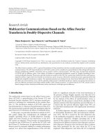
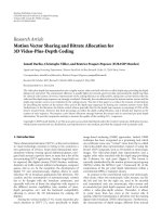
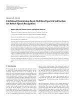
4. PROCESSOR IMPLEMENTATION

As mentioned in Section 3, the two main computing issues
lead to different architectural counterparts. The development
of a new function evaluation upon the previous one in a
spreading calculation scheme is carried out by the processor
presented in Figure 1 that requires function G to be known.
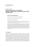
The second scheme deals with the crossed paired calculation
of the F and G func tions. The corresponding processor is
shown in Figure 2.
The implementation proposed uses an LRA (acronym
for look-up table (LUT), register, reduction structure, and
adder). T he LUT contains all partial products αA
k
+ βB
k
; A
k
,
B
k
are portions of few bits of the current input data F
i
and G
i
.
6 EURASIP Journal on Advances in Signal Processing
Table 5: Arithmetic processor estimations of area cost and time delay for 16 bits and one-bit fragmented data.
Hardware devices Occupied area Time delay
Multiplexer 0.25 ·×2 ×16τ
a
= 8τ

a
0, 5τ
t
Shift register 0.5 ×16τ
a
= 8τ
a
15 ×0,5τ
t
= 7, 5τ
t
LRA
LUT 40 τ
a
/Kbit ×16 bits × 16 cell = 10τ
a
3.5τ
t
× 16 accesses = 56τ
t
Register 0.5 ×16 · τ
a
= 8τ
a
1τ
t
Reduction structure 4 : 2 + adder 4τ
a
+16τ
a

= 20τ
a
3red.× 3τ
t
+lg16τ
t
= 13τ
t
Arithmetic processor (Figure 1) 70τ
a
78τ
t
Arithmetic processor (Figure 2) 108τ
a
78τ
t
Table 6: Relationship between area, time delay, and fragment length k, for 16 bits data for processor 2.
k = 1 k = 2 k = 4 k = 8 k = 16
LUT area 20τ
a
80τ
a
2048τ
a
524288τ
a
34359738368τ
a
LUT area versus
overall area

20τ
a
108τ
a
= 0.18
80τ
a
168τ
a
= 0.47
2048τ
a
2136τ
a
= 0.96
> 0.99 > 0.99
L UT time access 56τ
t
28τ
t
14τ
t
7τ
t
3τ
t
L UT time access
versus overall
processing time
56τ

t
78τ
t
= 0.72
28τ
t
50τ
t
= 0.56
14τ
t
36τ
t
= 0.39
7τ
t
29τ
t
= 0.24
3τ
t
25τ
t
= 0.12
On every cycle, the LUT is respectively accessed by A
k
and B
k
coming from the shift registers. Then, the partial products
are taken out of the cells (partial products in the LUT are the

hardware counterpart of the weighted primitives presented
in Tables 1 and 2). The overall partial product αF
i
+βG
i
is ob-
tained by adding all the shifted partial products correspond-
ing to all fragment inputs A
k
, B
k
of F
i
and G
i
,respectively.
In the following iteration, both the new calculated F
i+1
value
and the next G
i+1
value are multiplexed and shifted before
accessing the LUT in order to repeat the addressing process.
The processor in Figure 2 is different fr o m Figure 1 in what
concerns function G.TheG values are obtained in the same
way as for F but the LUT for G is different from the LUT for
F.
4.1. Area costs and time delay estimation
In order to have the capability to make a comparison of com-
puting resources, an estimation of the area cost and time

delay of the proposed architectures is presented here. The
model we use for the estimations is taken from the references
[33, 34]. The unit τ
a
represents the area of a complex gate.
The complex gate is defined as the pair (AND, XOR) that
provides a meaningful unit, as these two gates implement the
most basic computing device: the one bit full-adder. The unit
τ
t
is the delay of this complex gate. This model is ver y use-
ful because it provides a direct way to compare different ar-
chitectures, without depending on their implementation fea-
tures. As an example, the area cost and time delay for 16 bits
one-bit fragmented data are estimated for both processors, as
shown in Table 5.
If the fragments of the input data are greater than one bit,
then the occupied area and the time delay access of the LUT
vary. The relationship between area, time delay, and fragment
length k for 16 bits data is shown in Table 6 for processor 2.
Table 6 outlines that the LUT area increases exponentially
with k, and represents an increasing portion of the overall
area as k increases. The access time for the LUT decreases as
1/k. The percentage of access time versus overall processing
time decreases slowly as 1/k. The trade-off between area and
time has to be defined depending on the application.
The proposed architecture has also been tested in the
XS4010XL-PC84 FPGA. Time delay estimation in usual time
units can also be provided assuming τ
t

≈ 1ns.
4.2. Algorithmic stability
A complete study of the error is still under consideration and
numerical results are not yet available except for particular
cases [35]. Nevertheless, two main considerations are pre-
sented: on one hand, the recursive calculation accumulates
the absolute error caused by the successive round-off which
is performed as the number of iterations increases, on the
other hand, if round-off is not performed, the error can be-
come lower as the length in bits of the result increases, but
the occupied area as well as the time delay increase too. In
what follows, both trends are analyzed.
Round-off is performed
The drawback of the increasing absolute error can be faced
by decreasing the number of iterations, that is to say the
number of calculated values, with the corresponding loss of
Mar
´
ıa Teresa Signes Pont et al. 7
accuracy of the mapping. A trade-off between the accuracy
of the approximation (related to the number of calculated
values) and the increasing calculation error must be found.
Parallelization provides a mean to deal with this problem by
defining more computing levels. The N values of function F
that are to be calculated can be assigned to different com-
puting levels (therefore different computing processors) in a
tree-structured architecture, by spreading N into a product
as follows:
N
= N

1
· N
2
···N
P
. (11)
– 1st computing level: F
0
is the seed value that initializes
the calculation of N
1
new values,
– 2nd computing level: the N
1
obtained values are the
seeds that initialize the calculation of N
1
·N
2
new val-
ues (N
2
values per each N
1
).
And so on until achieving the
– pth computing level: the N
p−1
obtained values are
the seeds that complete the calculation of N

= N
1
·
N
2
···N
p
new values (N
p
values per each N
p−1
).
If the error for one v alue calculation is assumed to be ε,
the overall error after N values calculation is
– for sequential calculation
= Nε = N
1
· N
2
·····N
p
ε,
– for calculation by a tree structured architecture
=
(N
1
+ N
2
+ ···+ N
p

)ε.
The parallelized calculation decreases the overall error
without having to decrease the number of points. The min-
imum value for the overall error is obtained when the sum
(N
1
+ N
2
+ ···+ N
p
) is minimized, that is to say when all N
i
in the sum are relatively prime factors.
It can be mentioned that the time delay calculation fol-
lows a similar evolution scheme as the error. Considering T
as the time delay for one value calculation, the overall time
delay is
– for sequential calculation
= NT = N
1
·N
2
·····N
p
T,
– for calculation by a tree structured architecture
=
(N
1
+ N

2
+ ···+ N
p
)T.
The minimization of the time delay is also obtained when
the N
i
are relatively prime factors.
For the occupied area, the precise structure of the tree
in what concerns the depth (number of computing levels)
and the number of branches (number of calculated values
per processor) is quite relevant for the result. The distribu-
tion of the N
i
is crucial in the definition of some improving
tendencies. The number of processors P in the tree-structure
can be bounded as follows:
P
= 1+N
1
+ N
1
· N
2
+ N
1
· N
2
· N
3

+ ···+ N
1
· N
2
· N
3
·····N
p−1
< 1+(p − 1)
N
Np
.
(12)
P increases at the same rate as the number of computing
levels p, but the growth can be contained if N
p
is the maxi-
mum value of all N
i
, that is to say in the last computing level
p
− 1, the number of calculated values per processor is the
highest. It can be observed that the parallel calculation in-
volves much more processors than sequential one processor.
Summarizing the main ideas
(i) The parallel calculation provides benefits on error
bound and time delay whereas sequential calculation
performs better in what concerns area saving.
(ii) A trade-off must be established between the time de-
lay, the occupied area, and the approximation accuracy

(through the definition of the computing levels).
Round-off is not performed
As explained in Section 2, we assume the first input data
length is n, the data have been fragmented (n
= kt), and
the partial products in the cells are p bits long. If t accesses
have been performed to the table and t partial products have
to be added, the first result w ill be p + t + 1 bits long (t bits
represent the increase caused by the corresponding shifts
plus one bit for the last carry). The second value has to be
calculated in the same way so that the p + t + 1 bits of the
feedback data is k-fragmented and the process goes on. This
recursive algorithm can be formalized as follows:
Initial v alue n bits
= A
0
bits
1st calculated value
p + t +1bits
= p +
n
k
+1bits
= p +1+
A
0
k
bits
= A
1

bits
2nd calculated value p +1+
A
1
k
bits
··· ···
and so on.
Table 7 presents the data length evolution and the corre-
sponding error for n
= p = 16, 32, and 64 bits data, as well
as the number of calculated values that lead to the maximum
data length achievement.
It can be noticed that the increase of the number of bits
is bounded after a finite and rather low number of calculated
values that decreases as k grows. As usual, the error decreases
as the number of the data bits increases and the results are
improved in any case by small fragmentation (k
= 2). When
round-off is not performed, time delay and area occupation
increase because of the higher number of bits involved, so
Tables 5 and 6 should b e modified. It can be outlined that
small fragmentation makes error to decrease, but time delay
would increase too much. By increasing the fragment length
value, time delay improves but the er ror and the area cost
would make this issue infeasible. The trade-off between area,
time delay, and error must be set regarding to the application.
8 EURASIP Journal on Advances in Signal Processing
Table 7: Data length evolution and error versus number of calculated values for n = p = 16, 32, and 64 bits.
Initial data length (bits) Fragment length Final data length (bits) Le ngth increase rate Number of calculated values Error

16
k = 2 34 112% 9 2
−34
k = 4 23 44% 4 2
−23
k = 8 19 19% 2 2
−19
k = 16 18 12.5% 2 2
−16
32
k = 2 66 106% 10 2
−66
k = 4 44 37.5% 5 2
−44
k = 8 38 18.8% 4 2
−38
k = 16 35 9.4% 3 2
−35
k = 32 34 6.2% 2 2
−34
64
k = 2 130 103% 11 2
−130
k = 4 86 34.3% 6 2
−86
k = 8 74 15.6% 4 2
−74
k = 16 69 7.8% 4 2
−69
k = 32 67 4.7% 2 2

−67
k = 64 66 3.1% 2 2
−66
5. GENERIC CALCULATION SCHEME FOR
INTEGRAL TRANSFORMS
In this section, a generic calculation scheme for integral
transforms is presented. The DFT is taken as a paradigm and
some other transforms are developed as applications of the
DFT calculation.
5.1. The DFT as paradigm
Equation (13) is the expression of the one-dimensional dis-
creteFouriertransform.LetushaveN
= 2M = 2
n
,
F(u)
=
1
N
N−1

x=0
f (x)W
ux
2M
,whereW
N
= exp
−2jπ
N

.
(13)
The Cooley and Tukey algorithm segregates the FT in
even and odd fragments in order to perform the successive
folding scheme, as shown in (14):
F(u)
=
1
2

F
even
(u)+F
odd
(u)W
u
2M

,
F(u + M)
=
1
2

F
even
(u) − F
odd
(u)W
u

2M

,
F
even
(u) =
1
M
M−1

x=0
f (2x)W
ux
M
,
F
odd
(u) =
1
M
M−1

x=0
f (2x +1)W
ux
M
.
(14)
For any u
∈ [0, M[, the Cooley and Tukey algorithm

starts by setting the M initial two-point transforms. In the
second step M/2 four-point transforms are carried out by
combining the former transforms and so on till to reach the
last step, where one M-point transform is finally obtained.
For values of u
∈ [M, N[ no more extra calculations are re-
quired as the corresponding t ransforms can be obtained by
changing the sign, as shown by the second row in (14).
Our method enhances this process by adding a new seg-
regation held by both real (R) and imaginary (I) parts in or-
der to allow the crossed evaluation presented at the end of
Section 3. Due to the fact that two segretations are consid-
ered (even/odd, real/imaginary) there will be, for each u,four
transforms, which are R
p,q even
, R
p,q odd
, I
p,q even
,andI
p,q odd
where p, q denote the step of the process and the number
of the transform in the step, respectively, p
∈ [0, n −1], and
q
∈ [0, 2
n−1
− 1].
Equations (15), (16), and (17) show the first, the sec-
ond, and the last steps of our process, respectively, for any

u
∈ [0, M[. Parameters α
p
(u) = cos pπu/M and β
p
(u) =
sin pπu/M define the step p.Theu argument has been omit-
ted in (16)and(17) in order to clarify the expansion. In
the first step, M two-point real and imaginary transforms
are set in order to start the process. In the second step M/2
real and imaginary transforms are car ried out following the
calculation scheme shown in (9). At the end of the process,
one real and one imaginary M-point transform are achieved
and, without any more calculation, the result is deduced for
u
∈ [M, N[. As observed in (16)and(17), each step involves
the results of R and I obtained in the two previous steps;
therefore, in each step the number of equations is halved. Af-
ter the first step, a sum is added to the weighted primitive.
Thiscouldhaveaneffect on the LUT as the parameter set
becomes (α, β,1),
u
∈ [0, M[
R
0,0 even
(u) = f (0) + α
0
(u) f

2

n−1

,
R
0,1 odd
(u) = f

2
n−2

+ α
0
(u) f

2
n−2
+2
n−1

,
···
R
0,M−1odd
(u) = f

2+2
2
+ ···+2
n−2


+ α
0
(u) f

2+2
2
+ ···+2
n−2
+2
n−1

,
Mar
´
ıa Teresa Signes Pont et al. 9
I
0,0 even
(u) =−β
0
(u) f

2
n−1

,
I
0,1 odd
(u) =−β
0
(u) f


2
n−2
+2
n−1

,
···
I
0,M−1odd
(u) =−β
0
(u) f

2+2
2
+ ···+2
n−2
+2
n−1

,
(15)
R
1,0 even
= R
0,0 even
+ α
1
R

0,1 odd
− β
1
I
0,1 odd
= R
0,0 even
+ R
0,1 odd
⊕ I
0,1 odd
,
I
1,0 even
= I
0,0 even
+ β
1
R
0,1 odd
+ α
1
I
0,1 odd
= I
0,0 even
+ R
0,1 odd
⊕ I
0,1 odd

,
R
1,1 odd
= R
0,2 even
+ α
1
R
0,3 odd
− β
1
I
0,3 odd
= R
0,2 even
+ R
0,3 odd
⊕ I
0,3 odd
,
I
1,1 odd
= I
0,2 even
+ β
1
R
0,3 odd
+ α
1

I
0,3 odd
= I
0,2 even
+ R
0,3 odd
⊕ I
0,3 odd
,
···
R
1,M/2−1odd
= R
0,M/2even
+ α
1
R
0,M/2+1odd
− β
1
I
0,M/2+1odd
= R
0,M/2even
+ R
0,M/2+1odd
⊕ I
0,M/2+1odd
,
I

1,M/2−1odd
= I
0,M/2even
+ β
1
R
0,M/2+1odd
+ α
1
I
0,M/2+1odd
= I
0,M/2even
+ R
0,M/2+1odd
⊕ I
0,M/2+1odd
,
(16)
R
= R
n−1,0
= R
n−2,0 even
+ α
n−1
R
n−2,1 odd
− β
n−1

I
n−2,1 odd
= R
n−2,0 even
+ R
n−2,1 odd
⊕ I
n−2,1 odd
,
I
= I
n−1,0
= I
n−2,0 even
+ β
n−1
R
n−2,1 odd
+ α
n−1
I
n−2,1 odd
= I
n−2,0 even
+ R
n−2,1 odd
⊕ I
n−2,1 odd
,
(17)

u
∈ [M, N[
R
= R
n−1,0
= R
n−2,0 even
− α
n−1
R
n−2,1 odd
+ β
n−1
I
n−2,1 odd
= R
n−2,0 even
− R
n−2,1 odd
⊕ I
n−2,1 odd
,
I
= I
n−1,0
= I
n−2,0 even
− β
n−1
R

n−2,1 odd
− α
n−1
I
n−2,1 odd
= I
n−2,0 even
− R
n−2,1 odd
⊕ I
n−2,1 odd
.
(18)
The number of operations has been used as the main unit
to measure the computational complexity of the proposal.
The operation implemented by the weighted primitive has
been denoted as weighted sum WS, and the simple sum as
SS. The calculations take into account both real and imagi-
nary parts for any u value. The initial two-point transforms
are assumed to be calculated. An inductive scheme is used to
carry out the complexity estimations.
(i) N
= 4, n = 2, M = 2
F(0): 1 SS
F(1): 2 ×3 = 6WS
F(2): deduced from F(0), 1 SS
F(3): deduced from F(1), 2
× 1 = 2 WS (change of sign)
Overall: 8WSand2SS.
(ii) N

= 8, n = 3, M = 4
F(0): 3 SS
F(1), F(2) and F(3)
= 14 WS
F(4): 3 SS
F(5), F(6) and F(7)
= 2 × 3 = 6 WS (change of sign)
Overall: 20 WS and 6 SS.
(iii) N
= 16, n = 4, M = 8
F(0): 7 SS
F(1), F(2), F(3), , F(7)
= 30 WS
F(8): 7 SS
F(9), , F(15)
= 2 × 7 = 14 WS (change of sign)
Overall: 44 WS and 14 SS.
From these results two induced calculation formulas can
be proposed referring to the count of needed weighted sums
and simple sums,
WS(n)
= 2 × WS(n −1) + 4,
SS(n)
= 2 × SS(n − 1) + 2.
(19)
Proof. Starting from WS(1)
= 2andSS(1)= 0, for any n,
n>1, it may be assumed that
WS(n)
= 2(2n − 1) + (2n − 2) = 2n +1+2n − 4,

SS(n)
= 2n − 2.
(20)
By the application of the inductive scheme, after substi-
tuting n by n + 1 the formulas become
WS(n +1)
= 2n +2+2n +1− 4,
SS(n +1)
= 2n +1− 2.
(21)
Comparing the expressions for n and n +1,itcanbeno-
ticed that
WS(n +1)
= 2 × WS(n)+4,
SS(n)
= 2 × SS(n − 1) + 2.
(22)
The proposed formulas (see (19)) have been validated by
this proof.
Comparing with the Cooley and Tukey algorithm, where
M(n) is the number of multiplications and S(n) the number
of sums, we have
M(n +1)
= 2 × M(n)+2
n
,
S(n +1)
= 2 × S(n)+2
n+1
.

(23)
The contribution of the weighted primitive is clear as
we compar e (19)and(23). The quotient M(n)/ WS(n) in-
creases linearly versus n. The same occurs with the quotient
S(n)/ SS(n) but with a steeper slope. So, the weighted primi-
tive provides best results as n grows.
5.2. Other transforms
This calculation scheme can be applied to other tra nsforms.
As DHT and DCT/DST are DFT-related transforms, a com-
mon calculation scheme can be presented after we perform
some mathematical manipulations.
10 EURASIP Journal on Advances in Signal Processing
Hartley transform
Let H(u) be the discrete Hartley t ransform of a real function
f (x):
H(u)
=
1
N
N−1

x=0
f (x)

cos
2πux
N
+sin
2πux
N


,
where R(u)
=
1
N
N−1

x=0
f (x)cos
2πux
N
,
I(u)
=
1
N
N−1

x=0
f (x)sin
2πux
N
.
(24)
H(u) is the transformed sequence that can split into two
fragments: R(u) corresponds to the cosine part and I(u)to
the sine part. The whole previous development for the DFT
can be applied but the last stage has to perform an additional
sum of the two calculated fragments,

H(u)
= R(u)+I(u). (25)
The number of simple sums increases as one last sum
must be performed per each u value. Nevertheless, (19)suits
because only the initial value varies, SS(1)
= 2,
WS(n)
= 2 × WS(n −1) + 4,
SS(n)
= 2 × SS(n − 1) + 2.
(26)
Cosine/sine transforms
Let C(u) be the discrete cosine transform of a real function
f (x):
C(u)
= e(k)
N−1

x=0
f (x)cos(2x +1)
πu
2N
. (27)
C(u) is the transformed sequence that can split into two
fragmentsasfollows:
f (x)cos(2x +1)
πu
2N
= f (x)cos


πux
N
+
πu
2N

=
f (x)

cos
πux
N
cos
πu
2N
− sin
πux
N
sin
πu
2N

.
(28)
So that (27)leadsto(29)
C(u)
= e(k)
N−1

x=0

f (x)

cos
πux
N
cos
πu
2N
− sin
πux
N
sin
πu
2N

.
(29)
Then, cos[πu/2N]and
−sin[πu/2N] are constant values
for each u value and can lay outside the summation:
C(u)
= e(k)

α
u
N
−1

x=0
f (x)cos

πux
N
+ β
u
N
−1

x=0
f (x)sin
πux
N

,
where cos
πu
2N
= α
u
, −sin
πu
2N
= β
u
.
(30)
Both fragments, R(u) (for the cosine part) and I(u)(for
the sine part), can be carried out under the DFT calcula-
tion scheme and combined in the last stage by an additional
weighted sum:
C(u)

= α
u
R(u)+β
u
I(u). (31)
A similar result could be inferred for sine transform
with the following parameter values: cos(πu/2N)
= α
u
,
sin(πu/2N)
= β
u
.
The number of weighted sums increases because of the
last weighted sum that must be performed, see (31). The
equation has been modified as the constant value in WS(n)
varies. The reason is that the initial value WS(1)
= 3,
WS(n)
= 2 × WS(n −1) + 3,
SS(n)
= 2 × SS(n − 1) + 2.
(32)
Summarizing
The calculation based upon the DFT scheme leads to an easy
approach for the calculation of the DHT and the DCT/DST,
as expected. This scheme can be extended to other integral
transforms with trigonometric kernel.
6. COMPARISON WITH OTHER PROPOSALS

AND DISCUSSION
In this section, some hardware implementations for the cal-
culation of the DFT, DHT, and DCT are presented in order
to provide a comparison for the different performances in
terms of area cost, time delay, and stability.
6.1. DFT
The BDA proposal presented by Chien-Chang et al. [36]car-
ries out the DFT of variable length by controlling the ar-
chitecture. The single processing element follows the Cooley
and Tukey algorithm radix-4 and calculates 16/32/64 points
transform. When the number of points N grows, it can split
out into a product of two factors N
1
× N
2
in order to pro-
cess the transform in a row-column structure. Formally, the
four terms of the butterfly are set as a cyclic convolution that
allows performing the calculations by means of distributed
arithmetic based on blocks. The memory is partitioned in
blocks that store the set of coefficients involved in the mul-
tiplications of the butterfly. A rotator is added to control the
sequence of use of the blocks and avoids storing all the com-
binations of the same elements as in conventional distributed
arithmetic. This architecture improves memory saving in ex-
change for increasing the time delay and the hardware be-
cause of the extra rotator in the circuit. This proposal sub-
stitutes the ROM by a RAM in order to make more flexi-
ble the change of the set of coefficients wh en the length of
the Fourier transform varies. The processing column consists

of an input buffer, a CORDIC processor that runs the com-
plex multiplications followed by a parallel-serial register and
a rotator. Four RAM memories and sixteen accumulators im-
plement the distributed arithmetic. At last, four buffers are
Mar
´
ıa Teresa Signes Pont et al. 11
Table 8: Critical path of the basic calculation module in the BDA architecture.
Preprocessor P/S RAM Adder + Acc Post-processor 4-point DFT Overall
Time per column 13.71 ns 12.45 ns 14.06 ns 17.7 ns 10.35 ns 68.27 ns
Critical path
17.7 ns 17.7 ns 17.7 ns 17.7 ns 17.7 ns 88.5 ns
Table 9: Compar ison between the hardware needed by BDA and our architecture implementations.
N Devices implementing the DBA architecture Devi ces implementing our proposal
16
5buffers, 1 CORDIC processor, P/S-R,
1rotator,4(4
× 16) bits RAMs, 16 MAC
4MUX,4S-R,
2(64
× 16) bits LUTs
4 registers, 4 red-structures
4 adders
64
5buffers, 1 CORDIC processor, P/S-R,
1rotator,4(16
× 16) bits RAMs, 16 MAC
512
9buffers, 1 CORDIC processor, 2 P/S-R,
1rotator,8(8

× 16) bits RAMs, 32 MAC
1 transposition memory
4096
9buffers, 1 CORDIC processor, 2 P/S-R,
1rotator,8(16
× 16) bits RAMs, 32 MAC
1 transposition memory
Table 10: Comparison between the BDA and our architecture implementations in terms of τ
a
and τ
t
.
N
BDA architecture Our proposal
Area Time delay Area Time delay
1116 314τ
a
3.310
3
τ
t
336τ
a
1.248 10
3
τ
t
1164 344τ
a
13.210

3
τ
t
4.992 10
3
τ
t
1512 632τ
a
105.610
3
τ
t
39.936 10
3
τ
t
4096 672τ
a
844.810
3
τ
t
119.808 10
3
τ
t
needed to reorder the partial products that are involved in
the basic four points operation. The number of operations of
this proposal is O((N

1
/4M)W
L
)whereN
1
is the length of the
transform, M
= 4 in the design, and W
L
is the data length.
When the transform is longer as 64 points, N
1
is substituted
by the N
1
×N
2
. Tab le 8 shows the results obtained by the syn-
opsis implementation of the circuit that has been described
in Verilog HDL.
In order to compare the performance of our architecture
and that of the BDA, an estimation of the occupied area and
time delay is provided. The devices for both implementa-
tions are listed in Ta ble 9 and evaluated in terms of τ
t
and
τ
a
in Table 1 0. For the crossed evaluation scheme, the archi-
tecture is double because of the two segregations (even/odd

and real/imaginary); 64 cells LUTs are assumed as the param-
etersetis(α, β, 1). Data is 16 bits long for any proposal. In
Table 1 0, neither the rotator nor the CORDIC processor has
been considered in the BDA implementation because the ref-
erence does not facilitate any detail upon their structure. The
estimations of the time delay are based on the author’s indi-
cations and presented in terms of τ
a
and τ
t
units.
It can be observed that the BDA architecture is worse
than the crossed one in what concerns the occupied area be-
cause the BDA hardware needs to be increased stepwise when
the number of points of the transforms increases. The time
delay is lower for the crossed architecture than for the BDA
for the values of N that have been considered and will remain
lower for any N, because it achieves a linear growing in both
implementations.
Table 1 1 summarizes the hardware cost as well as the time
delay of proposals for the Fourier transform calculation pre-
sented by different authors [13, 37–40]. The four proposals
in the beginning of the list have based their design on sys-
tolic matrices, the following one on adders and the others on
distributed arithmetic (the DA is a generic distributed arith-
metic approach). At the end of the list appears our proposal.
Average computation time is indicated as

N
1

4

W
L


T
ROM
+2T
ADD
+ T
LATCH

. (33)
It appears that our proposal is the best in what concerns
the hardware resources but time delay has a linear growth
with respect to N (number of points of the transform) and
with the data precision. It can be remembered that parallel
architecture may present a better performance for this case.
6.2. DHT
As mentioned in Section 1, the DHT algorithms are typi-
cally less efficient (in terms of the number of floating-point
12 EURASIP Journal on Advances in Signal Processing
Table 11: Comparison between our proposal and other ones.
Memory Adders Multipliers
Shift
registers
P/S
registers
CORDIC

Average
calculation time
Chang and
Chen [37]
0 NN 6N 00
N
× (2T
mult
+
2T
add
+ T
latch
)
Fang and
Wu [38]
02N +6 N +4 6N 00
N
× (2T
mult
+
2T
add
+ T
latch
)
Murthy and
Swamy [39]
0 NN10N 00
N

× (2T
mult
+
2T
add
+ T
latch
)
Chan and
Panchanathan [13]
0 NN 8N 00
N
× (2T
mult
+
2T
add
+ T
latch
)
Chang et al.
[40]
4N − 4(RAM) 6N +7 0 4N − 20 0
N/2
× (T
sum
+
T
latch
+ T

add
)
DA design
N
4
x2(ROM)
N
2
4
05NN 0
W
L
× (T
ROM
+
2T
add
+ T
latch
)
BDA design
N
4
x2(ROM)
N
4
+4
03N
N
4

N
4
+4
N
×W
L
/4×(T
ROM
+
2T
add
+ T
latch
)
Our proposal
2 ×W
L
× 2
3
(ROM) 2 + 2 0 2 0 0
(3N/2
−2)×W
L
T
ROM
+
(N
− 1)W
L
× T

add
Table 12: Lowest known operation counts (real multiplications + additions) for power-of-two DHT and corresponding DFT algorithms
versus our proposal (weighted sums + simple sums).
Size N DHT (split-radix FHT) DFT (split-radix FFT) Our proposal
4 0+8= 80+6= 68+6= 14
8
2+22= 24 2 + 20 = 22 20 + 14 = 34
16
12 + 64 = 76 10 + 60 = 70 44 + 30 = 74
32
42 + 166 = 208 34 + 164 = 198 92 + 62 = 154
64
124 + 416 = 540 98 + 420 = 518 188 + 126 = 314
128
330 + 998 = 1328 258 + 1028 = 1286 380 + 254 = 634
256
828 + 2336 = 3164 642 + 2436 = 3078 764 + 510 = 1274
512
1994 + 5350 = 7344 1538 + 5636 = 7174 1532 + 1022 = 2554
1024
4668 + 12064 = 16732 3586 + 12804 = 16390 3068 + 2046 = 5114
operations) than the corresponding DFT algorithm special-
ized for real inputs (or outputs), as proved by Sorensen et
al. in 1987 [19]. To illustrate this, Ta ble 12 lists the lowest
known operation counts (real multiplications + additions)
for the DHT and the DFT for power-of-two sizes, as achieved
by the split-radix Cooley-Tukey FHT/FFT algorithm in both
cases. Notice that, depending on DFT and DHT implemen-
tation details, some of the multiplications can be traded for
additions or vice versa. The third column of the table esti-

mates the operation counts (weighted sums + simple sums)
to be performed by our proposal, following (19).
As expected, our proposal behaves better in what con-
cerns the operation counts than both the DHT algorithm and
the corresponding DFT algorithm specialized for real inputs
or outputs. With respect to the particular hardware imple-
mentations, as the DFT has already been compared above
with our proposal, the concluding remarks related to the
DHT have to be deduced.
Adetailedanalysisofthecomputationalcostandespe-
cially of the numerical stability constants for DHT is pre-
sented by Arico et al. in [23]. The authors base their re-
search on the close connection existing between fast DHT
algorithms and factorizations of the corresponding orthog-
onal Hartley matrices of length N, H
N
. They achieve a fac-
torization of the matrix H
N
into a product of sparse ma-
trices (at most, two nonzero entries per row and column)
that allows an iterative calculation of H
N
x,foranyx ∈ R
N
.
Since the matrices are sparse and orthogonal, the factoriza-
tion of H
N
generates a fast and low arithmetic cost DHT al-

gorithms. The intraconnection of Hartley matrices of types
(II), (III), and (IV) is expressed by means of other Hartley
matrix of type (I), H
N
(I), is pursued by means of twiddle ma-
trices T
N
and T

N
(that are direct sums of 1 and of rotation-
reflection matrices of order 2). Finally, factorization of H
N
(I)
is achieved requiring permutations, scaling operations, but-
terfly operations, and plane rotations with small angles.
Mar
´
ıa Teresa Signes Pont et al. 13
Table 13: Normwise forward stability of DHT-I (N) for 16, 32, and 64 bits data.
N log
2
(N) u = 2
−16
u = 2
−32
u = 2
−64
16 4 13.292163u = 2
3.74

2
−16
= 2
−19.74
13.292163u = 2
3.74
2
−32
= 2
−35.74
13.292163u = 2
3.74
2
−64
= 2
−67.74
32 5 17.722908u = 2
4.16
2
−16
= 2
−20.16
17.722908u = 2
4.16
2
−32
= 2
−36.16
17.722908u = 2
4.16

2
−64
= 2
−68.16
64 6 22.153605u = 2
4.48
2
−16
= 2
−20.48
22.153605u = 2
4.48
2
−32
= 2
−36.48
22.153605u = 2
4.48
2
−64
= 2
−68.48
128 7 2
4.75
2
−16
= 2
−20.75
2
4.75

2
−32
= 2
−36.75
2
4.75
2
−64
= 2
−68.75
256 8 2
4.97
2
−16
= 2
−20.97
2
4.97
2
−32
= 2
−36.97
2
4.97
2
−64
= 2
−68.97
512 9 2
5.16

2
−16
= 2
−21.16
2
5.16
2
−32
= 2
−37.16
2
5.16
2
−64
= 2
−69.16
1024 10 2
5.33
2
−16
= 2
−21.33
2
5.33
2
−32
= 2
−37.33
2
5.33

2
−64
= 2
−69.33
2048 11 2
5.49
2
−16
= 2
−21.49
2
5.49
2
−32
= 2
−37.49
2
5.49
2
−64
= 2
−69.49
4096 12 2
5.63
2
−16
= 2
−21.63
2
5.63

2
−32
= 2
−37.63
2
5.63
2
−64
= 2
−69.63
8192 13 2
5.75
2
−16
= 2
−21.75
2
5.75
2
−32
= 2
−37.75
2
5.75
2
−64
= 2
−69.75
16384 14 2
5.87

2
−16
= 2
−21.87
2
5.87
2
−32
= 2
−37.87
2
5.87
2
−64
= 2
−69.87
The computational complexity is calculated for all types
DHT-X, X
= I, II, III, and IV but for comparison with our
results we will consider the best result which is for X
= I.
The number of additions is denoted by α(DHT-I, N)and
the number of multiplications by μ(DHT-I, N):
(DHT-I, N)
=
3
2N
log
2
(N) −

3
2N
+2,
μ(DHT-I, N)
= N log
2
(N) − 3N +4.
(34)
As seen in the paper, the operation error follows the IEEE
precision arithmetic u
= 2
−24
or u = 2
−53
depending on the
precision of the mantissa (24 or 53 bits, resp.). The round-
off algorithmic errors are related to the structure of the in-
volved matrices and for direct calculation the round-off error
is evaluated as a squared distance bounded by an expression
≈ k
N
u. The numerical stability is measured by k
N
that can be
understood as the relative error on the output vector (of the
mapping previously defined). For any X, a different expres-
sion for k
N
is obtained for the corresponding DHT-X(N).
All k

N
expressions are similar and have linear dependence of
log
2
N. For example, the normwise forward stability for
DHT-I(N)is

4
3
√
3+
3
2
√
2


log
2
N −1

+ O(u)

u.
(35)
As far as we can compare this very deep and strong the-
oretical approach with our method that is rather empirical,
the results that can be taken into account are the computa-
tional cost and the stability of the algorithms. To make easier
the comparison with our paper in what concerns the num-

ber of operations to be performed, a recursive formulation
of (DHT-I, N)andμ(DHT-I, N)
= for N = 2
n
has been de-
duced from (34):
α(n)
= 2α(n − 1) + 3.2
n
− 2,
μ(n)
= 2μ(n − 1) + 2
n
− 4.
(36)
0
20
40
60
80
100
120
140
0 50 100 150 200
Log
2
(N)
s(n)
m(n)
Figure 3: Growing rates s(n)andm(n)versusn.

Table 14: Number of multiplication and addition operations for
different 4
× 4DCTs.
Operation
Fast algorithms
Our proposal
[48][49][47]
Multiplication 512 256 172 45
Addition
496 480 963 14
The initial values are for n =1, following (34):
α(1)
=
3
2
· 2.1 −
3
2
· 2+2= 2,
μ(1)
= 2 · 1 − 3+4= 3.
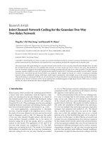
(37)
The comparison between (19)and(36)(WS(n)versus
μ(n) and SS(n)versusα(n)) outlines that α(n)andμ(n) in-
crease at a higher speed than WS(n) and SS(n), respectively,
(i) for all n, α(n) > SS(n),
(ii) for n>6, μ(n) > WS(n).
Figure 3 represents the growing rates s(n)
= α(n)/ SS(n)
and m(n)

= μ(n)/ WS(n)versusn.
The value of the normwise forward stability in the case of
DHT-I (N) is (((4/3)
√
3+(3/2)
√
2)(log
2
N −1) + O(u))u =
4.430721(log
2
N −1)u. In order to compare with our results
14 EURASIP Journal on Advances in Signal Processing
Table 15: Number of recursive cycles for different N × N DCT recursive structures.
N × N
Row-column method with transposition memory
Recursive
algorithm
Our
proposal
[42][43][45][46] [47]
Power of two
8 ×8 1024 1024 800 256 220 189
16 ×16 8192 8192 5952 2048 1756 765
32 ×32 65526 65536 45696 16384 14044 3069
64 ×64 524288 524288 357632 131073 112348 12285
128 ×128 4194304 4194304 2828800 1948567 898780 49149
Number of recursive kernels 1112 2 0
Size of transposition memory
O


N
2

O

N
2

O

N
2

O

N
2

0 0
Table 16: Comparison between the hardware needed by the recursive architecture versus that of the implementation of our proposal for
4
× 4DCTtransform.
N × N Devices implementing the recursive architecture Devices implementing our proposal
4 ×4
1 × Data memory buffer,
4 × MUX, 4 S-R,
2
×(64 ×16) bits LUTs
4

× registers,
4
× reduction structures
4
× adders
2 × adders
2 × 1–4 DEMUX
1 × CMP
1 × Condensed counter
(2
× ripple connected mod-4 counters)
1 × Condensed index generator
(2 S-R, 2 shifters, 3 adders)
2 × Recursive input buffer
2 × 1D DCT/DST IIR
of Table 7, the previous formula has been calculated for the
cases u
= 2
−16
,2
−32
,and2
−64
bits and for different values
of N.
The comparison between Tables 7 and 13 shows that for
16 bits (fragmentation lengths k
= 2andk = 4), for 32 bits
data (k
= 2, 4, and 8) and for 64 bits data (k = 2, 4, and 8)

our algorithm behaves better.
6.3. DCT
The search for recursive algorithms with regular structure
and less computation time remains an active research area.
The recursive algorithms for computing 1D DCT are highly
regular and modular [41–47]. However, a great number of
cycles are required to compute the 2D transformation by us-
ing 1D recursive structures. For computing the 2D DCT by
row-column approaches, the row (column) transforms of the
input 2D data are first determined. A tra nsposition mem-
ory is required to store those temporal results. Finally, the
2D DCT results are obtained by the column (row) trans-
forms of the transposed data. The RAM is usually adopted as
the transposition memory. This approach has disadvantages
such as higher-power consumption and long access time.
Chen et al. develop in 2004 a new recursive structure with fast
and regular recursion to achieve fewer recursive cycles with-
out using any tr a nsposition memory structure [48]. The 2D
recursive DCT/IDCT algorithms are developed considering
that the data with the same transform base can be pre-added
such that the recursive cycles can be reduced. First, the 2D
DCT/IDCT is decomposed into four portions which can be
carried out either by 1D DCT or 1D DST (discrete sine trans-
form). Based on the use of Chebyshev polynomials, efficient
transform kernels are obtained for the 1D DCT and the DST.
A reduction on the number or recursive cycles is achieved by
a further folding on the inputs of the transform kernels. Con-
sidering other fast algorithms, the N
× N DCT which maps
the 2D index of the input sequence into the new 1D index

is decomposed into N length-N 1D DCTs [49, 50]. Tab le 14
presents the number of multiplication and addition opera-
tions for these fast algorithms, for the case of 4
× 4DCTs.
Our proposal can be compared by assimilating the weighted
sums and the multiplications (see (32)).
The number of operations required for our proposal is
lower than those required for the existing methods. Table 1 5
shows the number of recursive cycles for different N
×N DCT
recursive structures in five different algorithms [43, 44, 46–
48]. In [48], a recursive cycle represents the time delay
needed for computing the 2D DCT cosine transform for
a pair of frequency indexes. The circuit involves two par-
allel identical block diagrams, both with a condensed 1D
DCT/DST IIR filter which obtains the corresponding input
data from a recursive input buffer in order to perform the
partial calculation of the transform. In the last stage, the
transform is recombined by a sum of the two partial results.
Mar
´
ıa Teresa Signes Pont et al. 15
So, the overall time delay for the 2D may be the same as for
the 1D and the comparison with our proposal can be done as
we assimilate the number of recursive cycles with the number
of weighted sums to be performed following (32).
It can be outlined that our proposal has a better perfor-
mance than the other ones, namely fast and recursive algo-
rithms, in what concerns the number of recursive cycles. In
[48] the chip area can be estimated as we depict the hardware

recursive circuitry. Table 1 6 summarizes the hardware de-
vices of the recursive architecture compared with our pro-
posal for 4
× 4DCTtransform.
It can be observed that the devices for the implementa-
tion of the recursive architecture are numerous. Therefore,
greater values for N
× N may imply an increase of the chip
area; the reason is the growth of the storing memory required
for the buffers and for the number of outputs of the demul-
tiplexer. Referenc e [48]doesnotoffer any estimation of the
time delay of the calculation. Our proposal implementation
is very simple and has no variation related to the amount of
devices when the number of calculated values varies. With
respect to the time delay of the calculation in [48], as far as
we can suppose, it can be estimated by analyzing the critical
path of the depicted circuit. It seems to be higher than our
proposal’s one.
7. CONCLUSIONS
This paper has presented an approach to the scalability prob-
lem caused by the exploding requirements of computing re-
sources in function calculation methods. The fundamentals
of our proposal claim that the use of a more complete prim-
itive, namely a weighted sum, converts the calculation of the
function values into a recursive operation defined by a two-
input table. The strength of the method is concerned with the
fact that the operation to be performed is the same for the
evaluation of different functions (elementary or not). There-
fore, only the table must be changed because it holds the fea-
tures of the concrete evaluated function in the parameter val-

ues. This method provides a linear computational cost when
some conditions are fulfilled. Image processing transforms
that involve combined trigonometric functions provide an
interesting application field. A generic calculation scheme
has been developed for the DFT as paradigm. Other image
transforms namely the DHT and the DCT/DST are analyzed
under the scope of the DFT. When comparing with other
well-known proposals, it has been confirmed that our ap-
proach provides a good trade-off between hardware resource
and time delay saving as well as encouraging partial results in
what concerns error contention.
REFERENCES
[1] R. Chamberlain, E. Lord, and D. J. Shand, “Real-time 2D
floating-point fast Fourier transfor m s for seeker simulation,”
in Technologies for Synthetic Environments: Hardware-in-the-
Loop Testing VII, R. L. Murrer Jr., Ed., vol. 4717 of Proceedings
of SPIE, pp. 15–23, Orlando, Fla, USA, July 2002.
[2] P.Yan,Y.L.Mo,andH.Liu,“Imagerestorationbasedonthe
discrete fraction Fourier transform,” in Image Matching and
Analysis, B. Bhanu, J. Shen, and T. Zhang, Eds., vol. 4552 of
Proceedings of SPIE, pp. 280–285, Wuhan, China, September
2001.
[3]W.A.Rabadi,H.R.Myler,andA.R.Weeks,“Iterativemul-
tiresolution algorithm for image reconstruction from the mag-
nitude of its Fourier transform,” Optical Engineering, vol. 35,
no. 4, pp. 1015–1024, 1996.
[4] C H. Chang, C L. Wang, and Y T. Chang, “Efficient VLSI
architectures for fast computation of the discrete Fourier
transform and its inverse,” IEEE Transactions on Signal Pro-
cessing, vol. 48, no. 11, pp. 3206–3216, 2000.

[5] S F. Hsiao and W R. Shiue, “Design of low-cost and high-
throughput linear arrays for DFT computations: algorithms,
architectures, and implementations,” IEEE Transactions on
Circuits and Systems II, vol. 47, no. 11, pp. 1188–1203, 2000.
[6] J. W. Cooley and J. W. Tukey, “An algorithm for the machine
calculation of complex Fourier series,” Mathematics of Com-
putation, vol. 19, no. 90, pp. 297–301, 1965.
[7] P. N. Swarztrauber, “Multiprocessor FFTs,” Parallel Comput-
ing, vol. 5, no. 1-2, pp. 197–210, 1987.
[8] C. Temperton, “Self-sorting in-place fast Fourier transforms,”
SIAM Journal on Scientific and Statistical Computing, vol. 12,
no. 4, pp. 808–823, 1991.
[9] M. C. Pease, “An adaptation of the fast Fourier transform for
parallel processing,” JournaloftheACM, vol. 15, no. 2, pp.
252–264, 1968.
[10] L. L. Hope, “A fast Gaussian method for Fourier transform
evaluation,” Proceedings of the IEEE, vol. 63, no. 9, pp. 1353–
1354, 1975.
[11] C L. Wang and C H. Chang, “A DHT-based FFT/IFFT pro-
cessor for VDSL transceivers,” in Proceedings of IEEE Interna-
tional Conference on Acoustics, Speech, and Signal Processing
(ICASSP ’01), vol. 2, pp. 1213–1216, Salt Lake, Utah, USA,
May 2001.
[12] W H. Fang and M L. Wu, “An efficient unified systolic archi-
tecture for the computation of discrete trigonometric trans-
forms,” in Proceedings of IEEE International Symposium on Cir-
cuits and Systems (ISCAS ’97), vol. 3, pp. 2092–2095, Hong
Kong, June 1997.
[13] E. Chan and S. Panchanathan, “A VLSI architecture for DFT,”
in Proceedings of the 36th Midwest Symposium on Circuits and

Systems, vol. 1, pp. 292–295, Detroit, Mich, USA, August 1993.
[14] R. V. L. Hartley, “A more symmetrical Fourier analysis applied
to transmission problems,” Proceedings of the IRE, vol. 30,
no. 3, pp. 144–150, 1942.
[15] R. N. Bracewell, “Discrete Hartley transform,” Journalofthe
Optical Society of America, vol. 73, no. 12, pp. 1832–1835,
1983.
[16] R. N. Bracewell, “The fast Hartley transform,” Proceedings of
the IEEE, vol. 72, no. 8, pp. 1010–1018, 1984.
[17] R. N. Bracewell, The Hartley Transform, Oxford University
Press, New York, NY, USA, 1986.
[18] R. N. Bracewell, “Computing with the Hartley t ransform,”
Computers in Physics, vol. 9, no. 4, pp. 373–379, 1995.
[19] H.V.Sorensen,D.L.Jones,M.T.Heideman,andC.S.Burrus,
“Real-valued fast Fourier transfer algorithms,” IEEE Transac-
tions on Acoustics, Speech, and Signal Processing, vol. 35, no. 6,
pp. 849–863, 1987.
[20] P. Duhamel and M. Vetterli, “Improved Fourier and Hartley
transform algorithms: application to cyclic convolution of real
data,” IEEE Transactions on Acoustics, Speech, and Signal Pro-
cessing, vol. 35, no. 6, pp. 818–824, 1987.
16 EURASIP Journal on Advances in Signal Processing
[21] M. Popovi
´
candD.
ˇ
Sevi
´
c, “A new look at the comparison of
the fast Hartley and Fourier transforms,” IEEE Transactions on

Signal Processing, vol. 42, no. 8, pp. 2178–2182, 1994.
[22] M. Frigo and S. G. Johnson, “The design and implementation
of FFTW3,” Proceedings of the IEEE, vol. 93, no. 2, pp. 216–231,
2005.
[23] A. Arico, S. Serra-Capizzano, and M. Tasche, “Fast and numer-
ically stable algorithms for discrete Hartley transforms and
applications to preconditioning,” Communications in Informa-
tion Systems, vol. 5, no. 1, pp. 21–68, 2005.
[24] K. R. Rao and P. Yip, Discrete Cosine Transform: Algorithms,
Advantages, Applications, Academic Press, Boston, Mass, USA,
1990.
[25] S. A. Martucci, “Symmetric convolution and the discrete sine
and cosine transforms,” IEEE Transactions on Signal Processing,
vol. 42, no. 5, pp. 1038–1051, 1994.
[26] W. B. Pennebaker and J. L. Mitchell, JPEG Still Image Data
Compression Standard, Van Nostrand Reinhold, New York, NY,
USA, 1993.
[27] Y. Q. Shi and H. Sun, Image and Video Compression for Multi-
media Engineering, CRC Press, Boca Raton, Fla, USA, 2000.
[28] P. Duhamel and C. Guillemot, “Polynomial transform com-
putation of the 2-D DCT,” in Proceedings of IEEE Interna-
tional Conference on Acoustics, Speech, and Signal Processing
(ICASSP ’90), vol. 3, pp. 1515–1518, Albuquerque, NM, USA,
April 1990.
[29] E. Feig and S. Winograd, “Fast algorithms for the discrete co-
sine transform,” IEEE Transactions on Signal Processing, vol. 40,
no. 9, pp. 2174–2193, 1992.
[30] A. C. Hung and T. H Y. Meng, “A comparison of fast in-
verse discrete cosine transform algorithms,” Multimedia Sys-
tems, vol. 2, no. 5, pp. 204–217, 1994.

[31] P. Duhamel and M. Vetterli, “Fast Fourier transforms: a tu-
torial review and a state of the art,” Signal Processing, vol. 19,
no. 4, pp. 259–299, 1990.
[32] S. Serra-Capizzano, “A note on antireflective boundary condi-
tions and fast deblurring models,” SIAM Journal on Scientific
Computing, vol. 25, no. 4, pp. 1307–1325, 2003.
[33] M. Ercegovac and T. Lang, Division and Square Root: Digit-
Recurrence, Algorithms and Implementations,Kl
¨
uwer Aca-
demic Publishers, Boston, Mass, USA, 1994.
[34] J A. Pi
˜
neiro, M. D. Ercegovac, and J. D. Bruguera, “High-radix
logarithm with selection by rounding,” in Proceedings of the
13th IEEE International Conference on Application-Specific Sys-
tems, Architectures and Processors (ASAP ’02), pp. 101–110, San
Jose, Calif, USA, July 2002.
[35] J. M. Garc
´
ıa Chamizo, M. T. Signes Pont, H. Mora Mora, and
G. de Miguel Casado, “Parametrizable architecture for func-
tion recursive evaluation,” in Proceedings of the 18th Confer-
ence on Design of Circuits and Integrated Systems (DCIS ’03),
Ciudad Real, Spain, November 2003.
[36] L. Chien-Chang, Ch. Chih-Da, and J. I. Guo, “A parameter-
ized hardware design for the variable length discrete Fourier
transform,” in Proceedings of the 15th International Conference
on VLSI De sign (VLSID ’02), Taiwan, China, August 2002.
[37] L. W. Chang and M. Y. Chen, “A new systolic array for discrete

Fourier transform,” IEEE Transactions on Acoustics, Speech,
and Signal Processing, vol. 36, no. 10, pp. 1665–1666, 1988.
[38] W H. Fang and M L. Wu, “An efficient unified systolic archi-
tecture for the computation of discrete trigonometric trans-
forms,” in Proceedings of IEEE International Symposium on
Circuits and Systems (ISCAS ’97), vol. 3, pp. 2092–2095, Hong
Kong, June 1997.
[39] N. R. Murthy and M. N. S. Swamy, “On the real-time compu-
tation of DFT and DCT through systolic architectures,” IEEE
Transactions on Signal Processing, vol. 42, no. 4, pp. 988–991,
1994.
[40] T S. Chang, J I. Guo, and C W. Jen, “Hardware-efficient
DFT designs with cyclic convolution and subexpression shar-
ing,” IEEE Transactions on Circuits and Systems II, vol. 47,
no. 9, pp. 886–892, 2000.
[41] V. Kober and G. Cristobal, “Fast recursive algorithms for
short-time discrete cosine transform,” Electronics Letters,
vol. 35, no. 15, pp. 1236–1238, 1999.
[42] L P. Chau and W C. Siu, “Recursive algorithm for the dis-
crete cosine transform with general lengths,” Electronics Let-
ters, vol. 30, no. 3, pp. 197–198, 1994.
[43] Z. Wang, G. A. Jullien, and W. C. Miller, “Recursive algorithms
for the for ward and inverse discrete cosine transform w ith ar-
bitrary length,” IEEE Signal Processing Letters,vol.1,no.7,pp.
101–102, 1994.
[44] M. F. Aburdene, J. Zheng, and R. J. Kosick, “Computation
of discrete cosine transform using Clenshaw’s recurrence for-
mula,” IEEE Signal Processing Letters, vol. 2, no. 8, pp. 155–156,
1995.
[45] Y H. Chan, L P. Chau, and W C. Siu, “Efficient implemen-

tation of discrete cosine transform using recursive filter struc-
ture,” IEEE Transactions on Circuits and Systems for Video Tech-
nology, vol. 4, no. 6, pp. 550–552, 1994.
[46] J F. Yang and C P. Fan, “Compact recursive structures for dis-
crete cosine transform,” IEEE Transactions on Circuits and Sys-
tems II, vol. 47, no. 4, pp. 314–321, 2000.
[47] J. L. Wang, C. B. Wu, D B. Liu, and J F. Yang, “Recursive ar-
chitecture for realizing modified discrete cosine transform and
its inverse,” in Proceedings of IEEE Workshop on Signal Process-
ing Systems (SIPS ’99), pp. 120–130, Taipei, Taiwan, October
1999.
[48] C H. Chen, B D. Liu, and J F. Yang, “Direct recur-
sive structures for computing radix-r two-dimensional
DCT/IDCT/DST/IDST,” IEEE Transactions on Circuits and
Systems I: Regular Papers, vol. 51, no. 10, pp. 2017–2030, 2004.
[49] N. I. Cho and S. U. Lee, “A fast 4
× 4DCTalgorithmforthe
recursive 2-D DCT,” IEEE Transactions on Signal Processing,
vol. 40, no. 9, pp. 2166–2173, 1992.
[50] N. I. Cho and S. U. Lee, “Fast algorithm and implementation
of 2-D discrete cosine transform,” IEEE Transactions on Cir-
cuits and Systems, vol. 38, no. 3, pp. 297–305, 1991.
Mar
´
ıa Teresa Signes Pont received the B.S.
degree in computer science from the In-
stitut National des Sciences Appliqu
´
ees de
Toulouse (France) and in Physics Univer-

sidad Nacional de Educaci
´
on a Distancia
(Spain) in 1978 and 1987, respectively. She
received the Ph.D. degree in computer sci-
ence from the University of Alicante in
2005. Since 1996, she is a member of the
Computer Technology and Computation
Department at the same university where she is currently an As-
sociate Professor and Researcher of Specialized Processors Archi-
tecture Laboratory. Her areas of research interest include computer
arithmetic, computational biology and the design of floating points
units, and approximation algorithms related to VLSI design.
Mar
´
ıa Teresa Signes Pont et al. 17
Juan Manuel Garc
´
ıa Chamizo received his
B.S. degree in physics at the University of
Granada (Spain) in 1980, and the Ph.D. de-
gree in computer science at the University
of Alicante (Spain) in 1994. He is currently
a Full Professor and Director of the Com-
puter Technology and Computation De-
partment at the University of Alicante. His
current research interests are computer vi-
sion, reconfigurable hardware, biomedical
applications, computer networks and architectures, and artificial
neural networks. He has directed several research projects related

to the above-mentioned interest areas. He is a member of a Span-
ish Consulting Commission on Electronics, Computer Science, and
Communications. He is also member and editor of some program
committee conferences.
Higinio Mora Mora received the B .S. degree
in computer science engineering and the
B.S. degree in business studies from Univer-
sity of Alicante, Spain, in 1996 and 1997, re-
spectively. He received the Ph.D. degree in
computer science from the University of Al-
icante in 2003. Since 2002, he is a member
of the Computer Technology and Compu-
tation Department at the same university
where he is currently an Associate Professor
and Researcher of Specialized Processors Architecture Laboratory.
His areas of research interest include computer arithmetic, the de-
sign of floating points units, and approximation algorithms related
to VLSI design.
Gregorio de Miguel Casado received the
B.S. degree in computer science engineering
and a master degree in business administra-
tion from the University of Alicante, Spain,
in 2001 and 2003, respectively. Since 2001,
he is a member of the research group I2RC
of the Computer Technology and Compu-
tation Department at the same university
where he is currently a Researcher of the
Specialized Processors Architecture Labora-
tory. His areas of research interest include formal VLSI design
methods, computable analysis, and computer arithmetic for the de-

velopment of arithmetic operators for scientific computing.