Báo cáo hóa học: " Research Article An Efficient Kernel Optimization Method for Radar High-Resolution Range Profile Recognition" docx

Hindawi Publishing Corporation
EURASIP Journal on Advances in Signal Processing
Volume 2007, Article ID 49597, 10 pages
doi:10.1155/2007/49597
Research Article
An Efficient Kernel Optimization Method for Radar
High-Resolution Range Profile Recognition
Bo Chen, Hongwei Liu, and Zheng Bao
National Key Laboratory for Radar Signal Processing, Xidian University, Xi’an 710071, Shaanxi, China
Received 15 September 2006; Accepted 5 April 2007
Recommended by Christoph Mecklenbr
¨
auker
A kernel optimization method based on fusion kernel for hig h-resolution range profile (HRRP) is proposed in this paper. Based
on the fusion of l
1
-norm and l
2
-norm Gaussian kernels, our method combines the different characteristics of them so that not only
is the kernel function optimized but also the speckle fluctuations of HRRP are restrained. Then the proposed method is employed
to optimize the kernel of kernel principle component analysis (KPCA) and the classification performance of extracted features is
evaluated via support vector machines (SVMs) classifier. Finally, experimental results on the benchmark and radar-measured data
sets are compared and analyzed to demonstrate the efficiency of our method.
Copyright © 2007 Bo Chen et al. This is an open access article distributed under the Creative Commons Attribution License, which
permits unrestricted use, distribution, and reproduction in any medium, provided the original work is properly cited.
1. INTRODUCTION
Radar automatic target recognition (RATR) is to identify
the unknown target from its radar-echoed signatures. Tar-
get high-range-resolution profile contains more detail tar-
get structure information than that of low-range-resolution
radar echoes, so it plays an important role in RATR commu-

nity [1–4]. As is known, radar HRRP is a strong function of
target aspect, and serious speckle fluctuation may exist when
target-radar orientation changes, which makes HRRP RATR
a challenge task. In addition, target may exist at any posi-
tion in real system, thus the position of an observed HRRP
in a time window will vary between measurements, and this
time-shift variation should be compensated when perform-
ing classification [1–4].
Kernel methods have been applied successfully in solving
various problems in machine learning community. A kernel-
based algorithm is a nonlinear version of linear algorithm
where, through a nonlinear function Φ(x), the input vector
x has been previously transformed to a higher dimensional
space F in which we only need to compute inner products
(via a kernel function). The attractiveness of such algorithms
stems from their elegant treatment of nonlinear problems
and their efficiency in high-dimensional problems. For the
HRRP recognition, there exists complex nonlinear relation
between targets due to the noncooperation and maneuvering
characteristic of targets. Therefore, kernel methods cannot be
directly applied to recognition unless the above three prob-
lems of influencing HRRP recognition can be solved, which
will significantly improve the classification performance [1].
Given two input vectors x and y, their inner product in
feature space, F, can be wr itten in the form of kernel K as
K(x, y)
=

Φ(x) · Φ(y)


. (1)
The popular kernel functions are Gaussian kernel K(x, y)
=
exp(−γx− y
2
)withγ>0 and polynomial kernel K(x, y) =
((x · y)+1)
p
with p ∈ N. The choice of the right embed-
ding is of crucial importance, since each kernel will create a
different structure in the embedding space. The ability to as-
sess the quality of an embedding is hence a crucial task in
the theory of kernel machines. Recently, Xiong et al. [5]pro-
pose an alternate method for optimizing the kernel function
by maximizing a class separability criterion in the empiri-
cal feature space. In this paper, we give an extension of the
method which can fuse multiple kernel f unctions. Then for
the HRRP recognition, the proposed method is employed to
combine the two Gaussian kernels based on l
1
-norm and l
2
-
norm distance to eliminate the speckle fluctuation. Unlike
other kernel mixture model, in our method every element
of a kernel matr ix has a different coefficient because of the
use of data-dependent kernel [6], which is the reason that we
call it fusion kernel. To show its performance, the method
is applied to optimize the kernel of KPCA for HRRP RATR
proposed by [1].

2 EURASIP Journal on Advances in Signal Processing
Finally, the classification performance of features ex-
tracted by optimized KPCA is evaluated via support vector
machines (SVMs) [7] based on the benchmark and radar-
measured HRRP datasets.
2. PROPERTIES OF RADAR HRRP
The radar works in the optics region, and the electromag-
netism characteristics of targets can be described by the scat-
tering center target model, which is widely used and also
proved to be a suitable target model in SAR and ISAR appli-
cations. An HRRP is the coherent sum of t ime returns from
target scatterers located within a range resolution cell, which
represents the distribution of target scattering centers along
the radar line of sight [3]. The mth complex returned echo in
the nthrangecellcanbewrittenas
x
n
(m) =
I
n

i=1
σ
n,i
exp

−
j

4πR

n,i
(m)
λ
+ θ
n,i

,(2)
where I
n
denotes the number of target scatterers in the nth
range cell, R
n,i
(m) denotes the distance between radar and
the ith scatterer in the mth sampled echo, σ
n,i
and θ
n,i
denote
the amplitude and initial phase of the ith scatterer echo, re-
spectively.
If the target orientation changes, its HRRP will be
changed subsequently. Two phenomena are responsible for
it. The first is the scatterer’s motion through range cell
(MTRC). Given target rotation angle larger enough, the scat-
terers range variation will be larger than a range resolution
cell, thus make the HRRP changed. Apparently the target ro-
tation angle, which leads to MTRC, is subjective to the range
resolution of radar and target-cross length. The second phe-
nomenon is the HRRP’s speckle effect. Since an HRRP is
the coherent summation of multiple scatterers echoes in one

range cell, even the target rotation angle meets the condition
of target rotation angle limitation to avoid the occurring of
MTRC, the phase of each scatterer echo will be changed, thus
their coherent summation will be changed subsequently.
If MTRC occurs, it means that the target scattering cen-
ter model changed. In this case, it is required more templates
to represent the target HRRPs. As to the speckle effect, an ef-
fective method of HRRP similarity scalar is needed to elim-
inate its influence on recognition performance, such as the
l
1
-norm distance [8].
3. FUSION KERNEL BASED ON l
1
-NORM AND
l
2
-NORM GAUSSIAN KERNELS
3.1. l
1
-norm and l
2
-norm Gaussian Kernels
Due to complicated nonlinear relations between radar tar-
gets, empirically Gaussian kernel is chosen to perform HRRP
recognition, which is proved by the empirical results in [1].
As the above, radar HRRP has the property of speckle effect
especially for propeller-driven aircraft, the running propeller
of which modulates the echoes and leads to the great fluc-
tuation of echoes. Usually, l

2
-norm Gaussian kernel is used,
which includes a square operation and augments the influ-
ence of the elements of large value in a vector, which will also
enhance the effect of speck fluctuation on recognition. Since
[8] shows us that l
1
-norm distance criterion can decrease the
fluctuation produced by propeller, l
1
-norm Gaussian kernel
can eliminate the speckle effect of HRRP,
K

X
1
(t), X
2
(t)

=
exp

−
γ


X
1
(t) − X

2
(t)


l
1

,(3)
where X
1
(t)andX
2
(t) denote two individual HRRPs, and γ is
a kernel parameter, which can be determined by a particular
criterion.
However, the useful information of HRRP exists in only
a part of all r ange cells and the rest are noise signal. Although
l
1
-norm distance can eliminate the speckle effect, the side
lobes also have been driven up, which means the increase of
the interference of the noise to signal. Whereas l
2
-norm dis-
tance can work well on decreasing the noise effect, so we ex-
pect to combine the two Gaussian kernels based on different
scales to learn a kernel function adaptive to HRRP data. In
the next section, a kernel optimization method will be given.
3.2. Kernel optimization based on fusion Kernel
in the empirical feature space

Although kernel-based methods such as KPCA [1]canrepre-
sent complex nonlinear relations among targets, the choices
of kernels and the kernel parameters still greatly influence
the classification performance. Obviously, a poor choice will
degrade the final results. Ideally, we select the kernel based
on our prior knowledge of problem domain and restrict the
learning to the task of selecting the particular pattern func-
tion in the feature space defined by the chosen kernel. Unfor-
tunately, it is not always possible to make the right choice of
kernel a priori. Furthermore, there is no general kernel suit-
able to all datasets. Therefore, it is necessary to find a data-
dependent objective function to evaluate kernel functions.
The method by Xiong et al. [5] employs a data-dependent
kernel similar to that used in [6]astheobjectivekerneltobe
optimized. In this section, we firstly review the kernel opti-
mization method.
3.2.1. Kernel optimization based on the single Kernel (SKO)
Given a two-class training data (x
1
, z
1
), (x
2
, z
2
), ,
(x
m
, z
m

) ∈ R
d
×{±1},wherex
i
∈ R
d
is the ith sample
and z
i
∈{±1} the label corresponding to x
i
. Given two data
samples x and y, a data-dependent kernel function is used,
k(x, y)
= q(x)q(y)k
0
(x, y), (4)
where x, y
∈ R
d
, k
0
(x, y), called the basic kernel, is an or-
dinary kernel such as a Gaussian or polynomial kernel, and
q(
·) is a factor function of the form
q(x)
= α
0
+

n

i=1
α
i
k
1

x, a
i

,(5)
where k
1
(x, a
i
) = e
−γ
1
x−a
i

2
, {a
i
∈ R
d
, i = 1, 2, , n}, called
the “empirical cores,” can be chosen from the training data
Bo Chen et al. 3

or local centers of the training data, and α
i
’s are the com-
bination coefficients which need normalizing. According to
[9, 10], evidently the data-dependent kernel satisfies the Mer-
cer condition for a kernel function.
The kernel matrices corresponding to k(x, y)andk
0
(x, y)
are denoted by K and K
0
,so(4)canberewrittenas
K
= QK
0
Q,(6)
where Q is a diagonal matrix, whose diagonal ele-
ments are
{q(x
1
), q(x
2
), , q(x
m
)}. We denote the vectors
(q(x
1
), q(x
2
), , q(x

m
))
T
,and(α
0
, α
1
, , α
n
)
T
by q and α,
respectively. Then, we have
q(α) =
⎛
⎜
⎜
⎜
⎜
⎝
1 k
1

x
1
, a
1

··· k
1


x
1
, a
n

1 k
1

x
2
, a
1

··· k
1

x
2
, a
n

.
.
.
.
.
.
.
.

.
.
.
.
1 k
1

x
m
, a
1

···
k
1

x
m
, a
n

⎞
⎟
⎟
⎟
⎟
⎠
⎛
⎜
⎜

⎜
⎜
⎝
α
0
α
1
.
.
.
α
n
⎞
⎟
⎟
⎟
⎟
⎠
=
K
1
α.
(7)
Here, the following quantity for measuring the class sepa-
rability is used as the kernel quality function in the empirical
feature space
J
=
trace


S
b

trace

S
w

,(8)
where S
b
=

2
i
=1
p
i
(μ
i
− μ)(μ
i
− μ)
T
is the “between-class
scatter matrix” and S
w
= (1/n)

n

i
=1
(x
i
− μ)(x
i
− μ)
T
the
“within-class scatter matrix,” μ is the global mean vector, μ
i
is the mean vector of ith class, and p
i
= n
i
/n is the prior of
ith class. It is obvious that optimizing the kernel through J
means increasing the linear separability of training data in
feature space so that the performance of kernel machines is
improved.
Now for the sake of convenience, we assume that the first
m
1
data belong to class C
1
, that is, z
i
= 1, i ≤ m
1
, and the

remaining m
2
data belong to C
2
(m
1
+ m
2
= m). Then, the
kernel matrix can be written as
K
=

K
11
K
12
K
21
K
22

,(9)
where K
11
, K
12
, K
21
,andK

22
represent the submatrices of K
of order m
1
× m
1
, m
1
× m
2
, m
2
× m
1
, m
2
× m
2
,respectively.
Now we can construct two kernel scatter matrices in the fea-
ture space as the fol lowing matrices:
B
=
⎛
⎜
⎜
⎜
⎝
1
m

1
K
11
0
0
1
m
2
K
22
,
⎞
⎟
⎟
⎟
⎠
−
⎛
⎜
⎜
⎜
⎝
1
m
K
11
1
m
K
12

1
m
K
21
1
m
K
22
⎞
⎟
⎟
⎟
⎠
,
W
=
⎛
⎜
⎜
⎜
⎜
⎜
⎜
⎜
⎝
k
11
0 ··· 0
0 k
22

··· 0
.
.
.
.
.
.
.
.
.
0
00
··· k
mm
⎞
⎟
⎟
⎟
⎟
⎟
⎟
⎟
⎠
−
⎛
⎜
⎜
⎝
1
m

1
K
11
0
0
1
m
2
K
22
⎞
⎟
⎟
⎠
.
(10)
Similarly, matr ices B
0
and W
0
correspond to the basic
kernel K
0
. According to [3, T heorem 1], we can use the kernel
scatter matrices to represent J,
J(α)
=
1
T
m

B1
m
1
T
m
W1
m
=
q(α)
T
B
0
q(α)
q(α)
T
W
0
q(α)
, (11)
where 1
m
is the vector of ones of the length m.
To maximize J(α), the standard gradient approach is em-
ployed and an updating equation for maximizing the class
separability J is given by the following:
α
(n+1)
= α
(n)
+ η


K
T
1
B
0
K
1
q

α
(n)

T
W
0
q

α
(n)

−
J

α
(n)

K
T
1

W
0
K
1
q

α
(n)

T
W
0
q

α
(n)


α
(n)
,
(12)
η is the learning rate and to ensure the convergence of the
algorithm, a gradually decreasing learning rate is adopted,
η(t)
= η
0

1 −
t

N

, (13)
where η
0
is the initial learning rate, N denotes a prespecified
number of iterations, and t the current iteration number.
We utilize artificially-generated data in two dimensions
in order to illustrate graphically the influence of kernel func-
tions on classification. Both class 1 (denoted by “
∗”) and
class 2 (“
◦”) were generated from mixtures of two Gaussians
by Ripley [11] with the classes overlapping to the extent that
the Bayes error is around 8.0% and the linear SVM error is
10.5%.
KPCA was used to extract feature with three initial “bad
guesses” of kernel matrices (Gaussian kernels with γ
= 10
and γ
= 0.25, polynomial kernel with p = 2. For nota-
tion simplification: the three kernels were respectively noted
as G10, G0.25, and P2) w hich were all normalized. Linear
SVM was used as a classifier. Figure 1(a) shows the orig-
inal distribution with 125-example training set (randomly
chosen from original Ripley’s 250). Figure 1(b) shows the
projection of training set in the Gaussian kernel (γ
= 10)
induced feature space. T he test error (the associated 1000-
example test s et) for KPCA

G10
(26.8%) is far inferior to
the original without KPCA which means it is a mismatched
kernel. Figure 1(c) shows the projection of the training set
through KPCA
G0.25
. The test error for KPCA
G0.25
(10.3%)
is slightly inferior to the original, which means a matched
kernel. Figure 1(d) shows the projection of the training set
through KPCA
P2
. The test error for KPCA
P2
(10.7%) is
slightly inferior to the original. Figures 1(e), 1(f), 1(g) show
the projections of the training set after SKO-KPCA
G10
,SKO-
KPCA
G0.25
, and SKO-KPCA
P2
.Avalueofγ
1
of the func-
tion k
1
(·, ·)in(3) for SKO-KPCA was selected using cross-

validation (CV). 50 fifty centers were selected to form the
empirical core set
{a
i
}. The initial learning r ate η
0
was set
to 0.01 and the total iteration number N
= 200. The test
errors for SKO-KPCA
G10
(25.6%), SKO-KPCA
G0.25
(9.4%),
4 EURASIP Journal on Advances in Signal Processing
−1.5 −1 −0.500.51
The first dimension
(a)
−0.2
0
0.2
0.4
0.6
0.8
1
1.2
The second dimension
−0.7 −0.5 −0.3 −0.10.10.30.50.7
The first principle component
(b)

−0.6
−0.4
−0.2
0
0.2
0.4
0.6
0.8
The second principle
component
−0.6 −0.4 −0.200.20.40.6
The first principle component
(c)
−0.4
−0.3
−0.2
−0.1
0
0.1
0.2
0.3
0.4
The second principle
component
−0.8 −0.6 −0.4 −0.20 0.20.40.60.8
The first principle component
(d)
−0.8
−0.6
−0.4

−0.2
0
0.2
0.4
0.6
The second principle
component
−0.7 −0.5 −0.3 −0.10.10.30.50.7
The first principle component
(e)
−0.6
−0.4
−0.2
0
0.2
0.4
0.6
0.8
The second principle
component
−0.15 −0.1 −0.05 0 0.05 0.10.15
The first principle component
(f)
−0.05
0
0.05
The second principle
component
−0.4 −0.200.20.4
The first principle component

(g)
−0.25
−0.2
−0.15
−0.1
−0.05
0
0.05
0.1
0.15
The second principle
component
Figure 1: Ripley’s Gaussian mixture data set and its projections in the empirical feature space onto the first two significant dimensions.
(a) The original training data set. (b)–(d) two-dimensional projections of the original training data set, respectively, in G10, G0.25, and P 2
kernel induced feature space. (e)–(g) two-dimensional projections of the original training data set, respectively, in G10, G0.25, and P2 kernel
induced feature space after the single kernel optimization.
Bo Chen et al. 5
and SKO-KPCA
P2
(10.1%) were superior to those before ker-
nel optimization.
However, we can see that the performance of SKO
method is very dependent on and limited by the initial se-
lected kernel. Which kernel function should b e selected to be
optimized, Gaussian kernel or other ones? How can we learn
abetterkernelmatrixfromdifferent kernels correspond-
ing to different physical interests adaptive to the input data?
Theseproblemsaredifficult to handle for the SKO method.
In the next section, we generalize the SKO method to a kernel
optimization algorithm based on fusion kernel (FKO).

3.2.2. Kernel optimization based on fusion Kernel (FKO)
It is evident that the method by Xiong et al. [5]iseffective
to improve the performance of the kernel machines, since
the targets are linearly separable in the feature space. Also
the experimental results in [5] prove it valid. Nevertheless,
the kernel optimization method is based on the single ker-
nel, which means that if a basic kernel function K
0
is cho-
sen beforehand, we have to optimize the kernel based on the
single embedding space, the optimization capability will be
limited consequentially. To generalize the method we extend
it to propose a more general kernel optimization approach
combining with the idea of fusion kernel mentioned in the
above.
If we choose L kernel functions, (6)canberepresentedas
K
=
L

i=1
Q
i
K
(i)
0
Q
i
, (14)
where K

(i)
0
is the ith basic kernel, Q
i
is the factor mat rix cor-
responding to K
(i)
0
. B and W are modified as
B
fusion
=
L

i=1
B
i
,
W
fusion
=
L

i=1
W
i
,
(15)
where
B

i
=
⎛
⎜
⎜
⎜
⎝
1
m
1
K
(i)
11
0
0
1
m
2
K
(i)
22
⎞
⎟
⎟
⎟
⎠
−
⎛
⎜
⎜

⎜
⎝
1
m
K
(i)
11
1
m
K
(i)
12
1
m
K
(i)
21
1
m
K
(i)
22
⎞
⎟
⎟
⎟
⎠
,
W
i

=
⎛
⎜
⎜
⎜
⎜
⎜
⎜
⎜
⎜
⎜
⎜
⎜
⎝
k
(i)
11
0 ··· 0
0 k
(i)
22
··· 0
.
.
.
.
.
.
.
.

.
0
00
··· k
(i)
mm
⎞
⎟
⎟
⎟
⎟
⎟
⎟
⎟
⎟
⎟
⎟
⎟
⎠
−
⎛
⎜
⎜
⎜
⎝
1
m
1
K
(i)

11
0
0
1
m
2
K
(i)
22
⎞
⎟
⎟
⎟
⎠
.
(16)
According to (11), the fusion kernel qualit y function
J
fusion
can be written as
J
fusion
=
1
T
m
B
fusion
1
m

1
T
m
W
fusion
1
m
=

L
i
=1
q
T
i
B
(i)
0
q
i

L
i=1
q
T
i
W
(i)
0
q

i
, (17)
where
q
i
=
⎛
⎜
⎜
⎜
⎜
⎜
⎜
⎝
1 k
1

x
1
, a
1

··· k
1

x
1
, a
n


1 k
1

x
2
, a
1

··· k
1

x
2
, a
n

.
.
.
.
.
.
.
.
.
.
.
.
1 k
1


x
m
, a
1

···
k
1

x
m
, a
n

⎞
⎟
⎟
⎟
⎟
⎟
⎟
⎠
⎛
⎜
⎜
⎜
⎜
⎜
⎜

⎜
⎝
α
(i)
0
α
(i)
1
.
.
.
α
(i)
n
⎞
⎟
⎟
⎟
⎟
⎟
⎟
⎟
⎠
=
K
1
α
(i)
.
(18)

The matr ices B
(i)
0
and W
(i)
0
correspond to the basic kernel
K
(i)
0
. α
(i)
is the combination coefficient vector corresponding
to K
(i)
0
.
Therefore, (17)canbederivedas
J
fusion
=
q
T
B
fusion
0
q
q
T
W

fusion
0
q
, (19)
where
B
fusion
0
=
⎡
⎢
⎢
⎢
⎢
⎢
⎢
⎢
⎣
B
(1)
0
0 ··· 0
0 B
(2)
0
··· 0
.
.
.
.

.
.
.
.
.
.
.
.
000B
(L)
0
⎤
⎥
⎥
⎥
⎥
⎥
⎥
⎥
⎦
,
W
fusion
0
=
⎡
⎢
⎢
⎢
⎢

⎢
⎢
⎢
⎣
W
(1)
0
0 ··· 0
0 W
(2)
0
··· 0
.
.
.
.
.
.
.
.
.
.
.
.
000W
(L)
0
⎤
⎥
⎥

⎥
⎥
⎥
⎥
⎥
⎦
,
q
=

q
1
q
2
··· q
L

=
⎡
⎢
⎢
⎢
⎢
⎢
⎢
⎣
K
1
0 ··· 0
0 K

1
··· 0
.
.
.
.
.
.
.
.
.
.
.
.
00
··· K
1
⎤
⎥
⎥
⎥
⎥
⎥
⎥
⎦
⎡
⎢
⎢
⎢
⎢

⎢
⎢
⎣
α
(1)
α
(2)
.
.
.
α
(L)
⎤
⎥
⎥
⎥
⎥
⎥
⎥
⎦
=
K
fusion
1
α
fusion
,
(20)
and K
fusion

1
is an Lm × L(n +1)matrix,α
fusion
is a vector of
length L(n +1).
Obviously, we can find that the form of (19) is the same
as that of the right-hand side of (11), so through (12), our
result can also be given by the following
α
fusion
(n+1)
= α
fusion
(n)
+ η


K
fusion
1

T
B
fusion
0
K
fusion
1
q


α
fusion
(n)

T
W
fusion
0
q

α
fusion
(n)

−
J
fusion

K
fusion
1

T
W
fusion
0
K
fusion
1
q


α
fusion
(n)

T
W
fusion
0
q

α
fusion
(n)


α
fusion
(n)
.
(21)
6 EURASIP Journal on Advances in Signal Processing
−0.15 −0.1 −0.05 0 0.05 0.10.15
The first principle component
−0.04
−0.03
−0.02
−0.01
0
0.01

0.02
0.03
0.04
The second principle component
(a)
0 50 100 150
Combination coefficient indices
−0.04
−0.02
0
0.02
0.04
0.06
Combination coefficients
G0.25
P2
G10
(b)
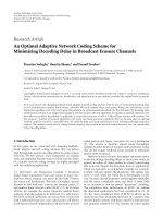
Figure 2: The results of Ripley’s data after FKO. (a) Two-dimensional projection of the training data in the optimized feature space. (b) the
combination coefficients α
fusion
.
When L = 1, it is just the single kernel optimization.
Figure 2(a) shows the projection of the training set in
the empirical feature space after the FKO. The parameters
were the same as those of the single kernel optimization. The
classifier was still linear SVM. The test error (9.0%) demon-
strates the improvement of the performance of the classifica-
tion. Meanwhile, shown in Figure 2(b) are the combination
coefficients of three initial kernels, α

fusion
.FromFigure 2(b),
we can clearly find that after kernel optimization, the combi-
nation coefficients of the mismatched kernel G0.1 have been
far less than other ones. Equivalently, our method automati-
cally selected G4 and P2 kernels to b e optimized, which both
match the Ripley’s data for classification.
4. EXPERIMENTAL RESULTS
4.1. Benchmark datasets
In order to evaluate the performance of our method, we
firstly test it on the four-benchmark datasets, namely, the
ionosphere, Pima Indians diabetes, liver disorder, wiscon-
sin breast cancer (WBC, where the 16 database samples with
missing values have been removed) which are downloaded
from the UCI benchmark repository [12]. Except Pima data
with training and test sets, in order to evaluate the true
performance, other data are randomly partitioned into two
equal and disjoint parts which are respectively used as train-
ing and test sets.
As the above, kernel optimization methods were ap-
plied to KPCA. Linear SVM classifier was utilized to evaluate
the classification performances. We used a Gaussian kernel
function, a polynomial kernel function K
2
(x, y) = ((x
T
· y)+
1)
p
, and a linear kernel function K

3
(x, y) = x
T
· y as ini-
tial basic kernel matrices. And all kernels were normalized.
Firstly, the values of kernel parameters for the three kernel
functions of KPCA without kernel optimization were respec-
tively selected by 10-fold cross-validation. Then the chosen
kernel functions were applied as the basis kernels in (4). σ
1
’s
in (5) were also selected using 10-fold cross-validation. 20 lo-
cal centers were selected to form the empirical core set
{a
i
}.
The initial learning rate η
0
was set to 0.08 and the total iter-
ation number T was set to 400. Meanwhile, the procedure of
determining the parameters of SKO was the same as FKO.
Experimental results on benchmark data are summarized
in Ta ble 1. It is evident that FKO can further improve the
classification performance and at least as the same as the SKO
method. The combination coefficients of three kernels in the
four experiments has also been illustrated in Figure 3.We
find that the combination coefficients of FKO are dependent
on the classification performance of the corresponding ker-
nel in SKO. As shown in Figure 3, the better the kernels can
work after the optimization of SKO, the larger the combina-

tion coefficientsofFKOare.Apparently,FKOcanautomati-
cally combine three fixed parameter kernels.
4.2. Measured high-resolution range profile (HRRP)
radar data set
The data used to further evaluate the classification perfor-
mance are measured from a C band radar with bandwidth
of 400 MHz. The radar high range resolution profile (HRRP)
data of three airplanes, including An-26, Yark-42, and Cessna
Bo Chen et al. 7
0102030405060
Combination coefficient indices
−0.2
−0.15
−0.1
−0.05
0
0.05
0.1
0.15
0.2
Combination coefficients
G
P
L
(a)
0102030405060
Combination coefficient indices
−0.08
−0.06
−0.04

−0.02
0
0.02
0.04
0.06
0.08
Combination coefficients
G
P
L
(b)
0102030405060
Combination coefficient indices
−0.06
−0.04
−0.02
0
0.02
0.04
0.06
0.08
0.1
Combination coefficients
G
P
L
(c)
0102030405060
Combination coefficient indices
−0.06

−0.04
−0.02
0
0.02
0.04
0.06
0.08
0.1
0.12
Combination coefficients
G
P
L
(d)
Figure 3: The combination coefficients corresponding to four datasets. (a) BCW; (b) pima; (c) liver; (d) ionosphere.
Citation S/II, are measured continuously when the targets are
flying. The projections of target trajectories onto the ground
plane are shown in Figure 4. The measured data of each tar-
get are divided into several segments, the training data and
test data are chosen from different data segments, respec-
tively, which means, the target orientations corresponding to
the test data and training data are different, the maximum
elevation difference between the test data and training data
is about 5 degrees. The 2nd and the 5th segments of Yark-42,
the 5th and the 6th segments of An-26, the 6th and the 7th
segments of Cessna Citation S/II are chosen as the training
data the total number of which is 300, all the rest data seg-
ments a re chosen as tests data, the total number of which is
2400. And in the kernel optimization, 50 local centers from
the training data are used as empirical cores. Additionally,

the original HRRPs are preprocessed by power transforma-
tion (PT) to improve the classification performance, which
is defined as
Y(t)
= X(t)
v
,0<v<1, (22)
8 EURASIP Journal on Advances in Signal Processing
−50 5
Km
0
20
40
60
Km
1
2
3
4
5
Radar
(a) Yark-42
−20 −15 −10 −50
Km
0
5
10
15
Km
3

2
1
4
5
6
7
7
Radar
(b) An-26
−20 −15 −10 −50
Km
0
5
10
15
Km
3
2
1
4
5
6
7
Radar
(c) Cessna Citation A/II
Figure 4: The projection of target trajectories onto the ground plane. (a) Yark-42, (b) An-26, (c) cessna citation S/II.
Table 1: The comparison of recognition rates of different methods
in different experiments. K
1
, K

2
,andK
3
, respectively, correspond to
Gaussian, polynomial, and linear kernels.
K
1
K
2
K
3
BCW
KPCA 88.96% 90.45% 88.58%
KPCA with SKO 88.96% 96.94% 97.1%
KPCA with FKO — 97.33%
Pima
KPCA 73.72% 64.15% 63.48%
KPCA with SKO 73.72% 66.21% 64.63%
KPCA with FKO — 74.10%
Liver
KPCA 71.19% 69.47% 66.19%
KPCA with SKO 74.67% 73.36% 73.47%
KPCA with FKO — 75.17%
Ionosphere
KPCA 93.11% 93.11% 89.73%
KPCA with SKO 93.11% 93.55% 89.38%
KPCA with FKO — 93.55%
where X(t) denotes an individual HRRP. The reason that
using PT can improve the classification performance is ex-
plained as that the nonnormality distributed original HRRPs

will become near normality distribution after PT, thus makes
the performance of many classifiers optimal. From HRRP
physical properties of view, PT amplifies the weaker echoes
and compresses the stronger echoes so as to decrease the
speckle effect in measuring the HRRPs similarity. The details
about PT can be referred to [13].
One-against-all linear SVM classifiers are trained for the
feature vectors extracted by SKO-KPCA, FKO-KPCA, and
KPCA without the kernel optimization, respectively. The pa-
rameters in the experiments are listed in Tabl e 2.Theexper-
imental results are shown in Figure 5, where the x-axis rep-
resents the number of principle components and the y-axis
the recognition rate.
In Figures 5(a)–5(c), each target recognition rates in dif-
ferent KPCA methods are shown respectively. Figure 5(d)
indicates the average recognition rates. From Figures 5(a)
and 5(d), we can find that KPCA w ith l
1
-norm and fusion
Table 2: The parameters in the experiment.
γ Empirical centers no. γ
1
η
0
Iteration no.
KPCA1 0.001
KPCA2 0.001
SKO-KPCA1 0.001 50 1 0.02 200
SKO-KPCA2 0.001 50 1 0.001 200
FKO-KPCA 0.001 50 1 0.0003 200

Note: KPCA1 and KPCA2 correspond to KPCA with l
1
-norm and
2-norm Gaussian kernels; SKO-KPCA1 and SKO-KPCA2
correspond to KPCA with l
1
-norm and 2-norm Gaussian kernels
after single kernel optimization; FKO-KPCA represents KPCA after
fusion kernel optimization based on l
1
-norm and 2-norm Gaussian
kernels.
Gaussian kernels perform better than with l
2
-norm Gaussian
kernel because of the different performances on An26. Due
to the modulability of the propeller of An26 on the HRRPs,
there still exists speckle effect even in a small angle sec-
tor. Therefore, l
1
-norm Gaussian kernel can be employed to
eliminate the large fluctuation so as to improve the recogni-
tion performance. By the fusion of l
1
-norm Gaussian kernel,
FKO-KPCA also works well. Meanwhile, Figure 5(d) shows
that the recognition rate of l
1
-norm Gaussian kernel SKO-
KPCA reaches 96.30% when the number of principle com-

ponent equals 140, while FKO-KPCA method only needs 90
components to reach its best classification rate 96.27%. Since
the fewer components mean lower computational complex-
ity, FKO-KPCA can extract effective features to reduce the
computational complexity in comparison KPCA with l
1
-
norm Gaussian kernel. Why can FKO-KPCA outperform
KPCA with l
1
-norm Gaussian kernel? In our opinion, the
possible reason is that when restricting the speckle effect, l
1
-
norm distance also augments the noise to interfere the sig-
nal, therefore, FKO-KPCA achieves better performance on
Cessna and Yark42 than KPCA with l
1
-norm Gaussian ker-
nel, as shown in Figures 5(b) and 5(c), which suggests that
our optimization method can adaptively combine the char-
acteristics of two kinds of kernels. From Figure 5(d),wecan
also observe that SKO-KPCA cannot effectively optimize the
Bo Chen et al. 9
20 40 60 80 100 120 140
Number of PCs
88
90
92
94

96
98
100
Recognition rates (%)
KPCA1
KPCA2
SKO-KPCA2
SKO-KPCA1
FKO-KPCA
(a)
20 40 60 80 100 120 140
Number of PCs
88
90
92
94
96
98
100
Recognition rates (%)
KPCA1
KPCA2
SKO-KPCA2
SKO-KPCA1
FKO-KPCA
(b)
20 40 60 80 100 120 140
Number of PCs
88
90

92
94
96
98
100
Recognition rates (%)
KPCA1
KPCA2
SKO-KPCA2
SKO-KPCA1
FKO-KPCA
(c)
20 40 60 80 100 120 140
Number of PCs
88
90
92
94
96
98
100
Recognition rates (%)
KPCA1
KPCA2
SKO-KPCA2
SKO-KPCA1
FKO-KPCA
(d)
Figure 5: Recognition rates on the measured radar HRRP data versus number of principle components in three experiments. (a) An-26 (b)
Cessna (c) Yark-42 (d) average recognition rates.

origin KPCA and l
1
-norm SKO-KPCA even decreased the
recognition rates.
5. CONCLUSIONS
In this paper, a kernel optimization method with learning
ability for radar HRRP recognition is proposed. The method
can adaptively combine the different characteristics of l
1
-
norm and l
2
-norm Gaussian kernels, so that not only is the
kernel function optimized but also the speckle fluctuations
of HRRP are restrained. Because of the use of kernel function
adaptive to data, each e lement in kernel matrix corresponds
to independent coefficient, which is the reason why it is called
fusion kernel optimization method. The classification per-
formance of features extracted by optimized KPCA are an-
alyzed and compared via support vector machines (SVMs)
based on benchmark and measured HRRP datasets, which
demonstrates the efficiency of our method.
10 EURASIP Journal on Advances in Signal Processing
ACKNOWLEDGMENT
This work is supported by the National Science Foundation
of China (no.60302009).
REFERENCES
[1] B. Chen, H. Liu, and Z. Bao, “PCA and kernel PCA for radar
high range resolution profiles recognition,” in Pro ceedings of
IEEE International Radar Conference, pp. 528–533, Arlington,

Va, USA, May 2005.
[2] B. Chen, H. Liu, and Z. Bao, “An efficient kernel optimiza-
tion method for high range resolution profile recognition,” in
Proceedings of IEEE International Radar Conference, pp. 1440–
1443, Shanghai, China, October 2006.
[3] L. Du, H. Liu, Z. Bao, and M. Xing, “Radar HRRP target recog-
nition based on higher order spectra,” IEEE Transactions on
Signal Processing, vol. 53, no. 7, pp. 2359–2368, 2005.
[4] L. Du, H. Liu, Z. Bao, and J. Zhang, “A two-distribution com-
pounded statistical model for radar HRRP target recognition,”
IEEE Transactions on Signal Processing, vol. 54, no. 6, pp. 2226–
2238, 2006.
[5] H. Xiong, M. N. S. Swamy, and M. O. Ahmad, “Optimizing
the kernel in the empirical feature space,” IEEE Transactions
on Neural Networks, vol. 16, no. 2, pp. 460–474, 2005.
[6] S. Amari and S. Wu, “Improving support vector machine
classifiers by modifying kernel functions,” Neural Networks,
vol. 12, no. 6, pp. 783–789, 1999.
[7] V. Vapnik, The Nature of Statistical Learning Theory, Springer,
New York, NY, USA, 1995.
[8] Z. Bao, M. Xing, and T. Wang, Radar Imaging Technique, Pub-
lishing House of Electronics Industry, Beijing, China, 2005.
[9] B. Sch
¨
olkopf, S. Mika, C. J. C. Burges, et al., “Input space ver-
sus feature space in kernel-based methods,” IEEE Transactions
on Neural Networks, vol. 10, no. 5, pp. 1000–1017, 1999.
[10] J. Shawe-Taylor and N. Cr istianini, Kernel Methods for Pattern
Analysis, Cambridge University Press, Cambridge, UK, 2004.
[11] B. D. Ripley, Pattern Recognition and Neural Networks,Cam-

bridge University Press, Cambridge, UK, 1996.
[12] C. Blake, E. Keogh, and C. J. Merz, “UCI repository of ma-
chine learning databases,” Tech. Rep., Department of In-
formation and Computer Science, University of California,
Irvine, Calif, USA, 1998. />∼mlearn/
MLRepository.html.
[13] H. Liu and Z. Bao, “Radar HRR profiles recognition based on
SVM with power-transformed-correlation kernel,” in Proceed-
ings of International Symposium on Neural Networks (ISNN
’04), vol. 3173 of Lecture Notes in Computer Science, pp. 531–
536, Dalian, China, August 2004.
Bo Chen received his B.Eng. and M.Eng. de-
grees in elect ronic engineer ing from Xidian
University in 2003 and 2006, respectively.
He is currently a Ph.D. student in the Na-
tional Key Lab of Radar Signal Processing,
Xidian University. His research interests in-
clude radar signal processing, radar auto-
matic target recognition, kernel machine.
Hongwei Liu received his M.S. and Ph.D.
degrees all in electronic engineering from
Xidian University in 1995 and 1999, respec-
tively. He joined the National Key Lab of
Radar Signal Processing, Xidian University
since 1999. From 2001 to 2002, he is a vis-
iting scholar at the department of electri-
cal and computer engineering, Duke Uni-
versity, USA. He is currently a Professor and
Director of National Key Lab of Radar Sig-
nal Processing, Xidian University. His research interests are radar

automatic target recognition, radar signal processing, and adaptive
signal processing. He is with the Key Laboratory for Radar Signal
Processing, Xidian University, Xi’an, China.
Zheng Bao graduated from the Communi-
cation Engineering Institution of China in
1953. Currently, he is a Professor at Xid-
ian University and an Academician of the
Chinese Academy of Science. He is the au-
thor or coauthor of six books and has pub-
lished more than 300 papers. Now his re-
search work focuses on the areas of space-
time adaptive processing, radar imaging,
and r adar automatic target recognition. He
is with the Key Laboratory for Radar Signal Processing, Xidian Uni-
versity, Xi’an, China.