Báo cáo hóa học: "Spin dynamics of an ultra-small nanoscale molecular magnet" potx
Bạn đang xem bản rút gọn của tài liệu. Xem và tải ngay bản đầy đủ của tài liệu tại đây (949.23 KB, 7 trang )
NANO EXPRESS
Spin dynamics of an ultra-small nanoscale molecular magnet
Orion Ciftja
Published online: 6 March 2007
Ó to the authors 2007
Abstract We present mathematical transformations
which allow us to calculate the spin dynamics of an ultra-
small nanoscale molecular magnet consisting of a dimer
system of classical (high) Heisenberg spins. We derive
exact analytic expressions (in integral form) for the time-
dependent spin autocorrelation function and several other
quantities. The properties of the time-dependent spin
autocorrelation function in terms of various coupling
parameters and temperature are discussed in detail.
Keywords Spin dynamics Á Nanoscale molecular
magnetism Á Time-dependent spin autocorrelation
function Á Exchange interaction Á Biquadratic exchange
interaction
Pacs numbers 75.10.Hk Á 75.50.Xx
Recent succesful efforts in synthesizing solid lattices of
weakly coupled molecular clusters containing few strongly
interacting spins has opened up the possibility of experi-
mentally studying magnetism at the nano scale [1]. Due to
the presence of organic ligands which wrap the molecular
clusters, the inter-cluster magnetic interaction is vanish-
ingly small when compared to intra-cluster interactions,
therefore the properties of the bulk sample reflect the
properties of independent individual nanoscale molecular
clusters. The magnetic ions in each molecular cluster can
be generally arranged in different ways, giving rise to
structures of very high symmetry (for example rings) and/
or of lower symmetry presenting other important features.
In some cases, the positions of the magnetic ions in the
cluster define a nearly planar ring structure within the host
lattice, for instance the Fe6 molecule is one of this type [2].
Here, the six Fe
3+
ions have spin S = 5/2 and are coupled
by nearest-neighbor antiferromagnetic exchange interac-
tions. Other nanoscale molecular clusters consist of para-
magnetic ions whose positions define a three-dimensional
structure. Examples of this type are the molecules Fe4 and
Cr4, which feature four Fe
3+
ions [3](S = 5/2) and four
Cr
3+
ions [4](S = 3/2), respectively, which occupy the
vertices of a tetrahedron embedded in the host lattice.
Smaller clusters are the irregular triangle molecule [5]
known as Fe3 which incorporates three Fe
3+
ions with spin
S = 5/2 and the dimer [6] system, Fe2 consisting of two
Fe
3+
ions with spin S = 5/2.
Low nuclearity complexes, such as Fe2 and Fe3, are
likely to represent the ‘‘molecular’’ nanoscale bricks for
the formation of high-nuclearity molecular clusters.
Therefore, their characterization is an essential step for
broader studies targeting larger systems [7]. Because of
the high spin value of the Fe
3+
ions, it turns out that the
measured magnetic susceptibility and other related quan-
tities can be reproduced to very high accuracy [8]by
using the classical Heisenberg model which incorporates
interaction between classical unit vectors. Only for very
low temperatures need one consider the quantum char-
acter of the Fe
3+
spins.
The spin dynamics of these nanoscale magnetic clusters
is of particular interest since it can directly be probed by
different experimental methods such as nuclear magnetic
resonance (NMR) [9]. In view of the importance of
knowing the dynamical behavior of spin–spin correlation
The author wants to thank Dr. Gary Erickson for proof-reading the
final draft of the paper.
O. Ciftja (&)
Department of Physics, Prairie View A&M University, Prairie
View, TX 77446, USA
e-mail:
123
Nanoscale Res Lett (2007) 2:168–174
DOI 10.1007/s11671-007-9049-5
functions it is most desirable to find model systems which
can be solved exactly. This way one can test the regimes of
validity of various experimental results and theoretical
approximation schemes. Among the variety of spin–spin
correlation functions, the time-dependent spin autocorre-
lation function is closely linked with spin dynamics,
therefore, it is natural to focus on this quantity. Earlier
studies have numerically investigated the time-dependent
spin autocorrelation function of many-spin systems such as
a classical Heisenberg model with nearest-neighbor ex-
change interaction between spins [10]. The goal of these
simulations was the study of the expected power-law decay
of the long-time spin autocorrelation function for many-
spin systems at infinite temperature [11].
In this work, we focus on the spin dynamics of ultra-
small, nanoscale, molecular magnets of classical (high)
Heisenberg spins. In particular, we give exact expressions
(in integral form) for the time-dependent spin autocorrela-
tion function at arbitrary temperature for a dimer system of
classical (high) spins that interact with both exchange and
biquadratic exchange interaction. The mathematical diffi-
culty to solve exactly the equations of motion and to per-
form the phase–space average for interacting spins makes
an exact analytical calculation of the time-dependent spin
autocorrelation function very challenging, even for the ul-
tra-small system considered here. To overcome these
mathematical difficulties we introduce a method which
simplifies the calculation of various quantities through the
introduction of suitably chosen auxiliary time-independent
variables into an extended phase–space integration [12, 13].
The present analytic results, although derived for the dimer
system of spins [14], can provide useful benchmarks for
assesing numerical methods that calculate the time-depen-
dent spin dynamics of other magnetic high-spin systems.
The Hamiltonian of a dimer system of spins with ex-
change and biquadratic interaction is written as
HðtÞ¼J
~
S
1
ðtÞ
~
S
2
ðtÞþK
~
S
1
ðtÞ
~
S
2
ðtÞ
hi
2
; ð1Þ
where J, K represent, respectively, the exchange, biquadratic
exchange interaction and
~
S
i
ðtÞ are time-dependent classical
spin vectors of unit length (i = 1,2). The orientation of the
classical unit vectors
~
S
i
ðtÞat a moment of time, t,isspecifiedby
polar and azimuthal angles, h
i
(t)and/
i
(t), which, respectively,
extend from 0 to p and0to2p. The exchange interaction
between a pair of spins can be either antiferromagnetic (AF),
J =|J| > 0, or ferromagnetic (F), J =–|J| < 0. The biquadratic
exchange interaction, K, can be positive, zero or negative.
At an arbitrary temperature, T, the time-dependent spin
autocorrelation function, C
T
ðtÞ¼h
~
S
i
ð0Þ
~
S
i
ðtÞi , is evaluated
as a phase space average over all possible initial time
orientations of the spins:
C
T
ðtÞ¼
R
d
~
S
1
ð0Þ
R
d
~
S
2
ð0Þexp ÀbHð0Þ½
~
S
i
ð0Þ
~
S
i
ðtÞ
ZðTÞ
; ð2Þ
where i = 1 or 2 is a selected spin index,
d
~
S
j
ð0Þ¼dh
j
ð0Þsin½h
j
ð0Þdu
j
ð0Þ is the initial time solid
angle element appropriate for the j-th spin, b = 1/(k
B
T),
and k
B
is Boltzmann’s constant. The denominator of
Eq. 2 represents the partition function, ZðTÞ¼
R
d
~
S
1
ð0Þ
R
d
~
S
2
ð0Þexp ÀbHð0Þ½, where H(0) is the initial time
Hamiltonian of the spin system. In order to evaluate the
time-dependent spin autocorrelation function we need first
to solve the equations of motions for the spins and then
perform the angular average over all possible initial time
spin orientations in the phase space.
The dynamics (equations of motion) of classical spins is
determined from
d
dt
~
S
i
ðtÞ¼À
~
S
i
ðtÞÂ
@HðtÞ
@
~
S
i
ðtÞ
; ð3Þ
where the set of solutions, f
~
S
i
ðtÞg depends on the initial
orientation of the spins, f
~
S
i
ð0Þg.
The calculation of C
T
(t) follows several steps: (i) solve
the equations of motion for the spins to obtain
~
S
i
ðtÞ; (ii)
calculate the partition function Z(T); and (iii) compute the
integrals appearing in the numerator of Eq. 2.
By applying Eq. 3 to each spin of the dimer, it is not
difficult to note that the total spin,
~
SðtÞ¼
~
S
1
ðtÞþ
~
S
2
ðtÞ,isa
constant of motion,
~
SðtÞ¼
~
Sð0Þ¼
~
S , and as a result we
can rewrite Eq. 3 as
d
dt
~
S
i
ðtÞ¼À½J þ KðS
2
À 2Þ
~
S
i
ðtÞÂ
~
S; ð4Þ
where
~
S represents the constant total spin.
The above differential equations for spins can be exactly
solved in a new coordinate system (x¢ y¢ z¢) in which the
constant vector
~
S lies parallel to the z¢ axis. Let us denote
(a
i
,b
i
) to be the polar and azimuthal angles of spin
~
S
i
ð0Þ
with respect to the new coordinate system in which the
direction of
~
S defines the z¢ (polar) axis. It follows that
S cosða
i
Þ¼
~
S
i
ð0Þ
~
S. The solution of Eq. 4 for each spin
component of
~
S
i
ðtÞ depends on the sign of [J + K (S
2
–2)].
Irrespective of the sign of [J + K (S
2
–2)], we find that the
quantity
~
S
i
ð0Þ
~
S
i
ðtÞ is given by the expression
~
S
i
ð0Þ
~
S
i
ðtÞ¼sin
2
ða
i
Þcos xðSÞt½þcos
2
ða
i
Þ; ð5Þ
where x(S)=|J + K (S
2
–2)| S denotes a precession fre-
quency, and 0 S ¼j
~
Sj 2 . Note that
~
S
i
ð0Þ
~
S
i
ðtÞ does not
depend on the i-th spin azimuthal angle b
i
.
In as much as the spins are equivalent, without loss of
generality we fix i = 1 and concentrate on the calculation
Nanoscale Res Lett (2007) 2:168–174 169
123
of C
T
ðtÞ¼h
~
S
1
ð0Þ
~
S
1
ðtÞi. From the definition of the total
spin variable,
~
S ¼
~
S
1
ð0Þþ
~
S
2
ð0Þ, recalling that S cosða
1
Þ¼
~
S
1
ð0Þ
~
S, we easily find that 1 þ
~
S
1
ð0Þ
~
S
2
ð0Þ¼S cosða
1
Þ.
Since the product
~
S
1
ð0Þ
~
S
2
ð0Þ is expressable in terms of the
total spin as
~
S
1
ð0Þ
~
S
2
ð0Þ¼S
2
=2 À 1, it follows that
cosða
1
Þ¼S=2, and it depends only on the total spin
magnitude. Through these simple mathematical transfor-
mations we reach the first goal to express
~
S
1
ð0Þ
~
S
1
ðtÞ as
~
S
1
ð0Þ
~
S
1
ðtÞ¼Fðt; SÞ¼ 1 À
S
2
4
cos xðSÞt½þ
S
2
4
: ð6Þ
In the same way, the Hamiltonian can be written in terms
of the total spin variable as
HðtÞ¼Hð0Þ¼
J
2
S
2
À 2
ÀÁ
þ
K
4
S
2
À 2
ÀÁ
2
ð7Þ
and is a constant of motion.
By expressing all relevant quantities in terms of the total
spin variable which is a constant of motion, we now apply
our calculation method whose success is based on the
observation that the values of all multi-dimensional inte-
grals, for example Z(T), are left unchanged if multiplied by
unity written as
Z
d
3
S
Z
d
3
q
ð2pÞ
3
exp i
~
q
~
S À
~
S
1
ð0ÞÀ
~
S
2
ð0Þ
hi
¼ 1: ð8Þ
Note that the above identity originates from the well known
formula,
R
d
3
Sd
ð3Þ
~
S À
~
S
1
ð0ÞÀ
~
S
2
ð0Þ
hi
¼ 1, that applies to
three-dimensional Dirac delta functions. Subsequent
calculations are straightforward given that both H(0) and
~
S
1
ð0Þ
~
S
1
ðtÞ appearing in Eq. 2 can be expressed solely in
terms of S. As a result, the integrations over individual spin
variables pose no problems. For the partition function, we
obtain
ZðTÞ¼ð4pÞ
2
Z
2
0
dSDðSÞexp À
bJ
2
S
2
À2
ÀÁ
À
bK
4
S
2
À2
ÀÁ
2
!
;
ð9Þ
where DðSÞ¼4pS
2
R
d
3
q
ð2pÞ
3
expði
~
q
~
SÞ sinq=qðÞ
2
can be
calculated analytically and is
DðSÞ¼
S=20\S\2
S=4 S ¼ 2
0 S[2
8
<
:
ð10Þ
The vanishing of D(S) for S > 2 reflects the constraint that
the total spin cannot exceed 2. Note that for K ” 0, the
partition function becomes ZðTÞ¼ð4pÞ
2
sinhðbJÞ
bJ
. In the
most general case, J „ 0 and K „ 0, the integral in
Eq. 9 can be expressed analytically in terms of error
functions. From the perspective of numerical calculations,
the above one-dimensional integral form is better suited.
The integral appearing in the numerator of Eq. 2 is
generally very difficult to calculate. However, using the
method illustrated above, integration is simplified, and one
obtains
C
T
ðtÞ¼
ð4pÞ
2
ZðTÞ
Z
2
0
dS DðSÞexp
À
bJ
2
ðS
2
À 2ÞÀ
bK
4
:
ðS
2
À 2Þ
2
!
Fðt; SÞ:
ð11Þ
The integrals appearing in Eq. 11 can be carried out ana-
lytically. The final result can be written in a closed form in
terms of error functions. The expressions are quite lengthy
and cumbersome. Because of such undesired complexity,
the one-dimensional integral representation in Eq. 11 not
only suffices, but is preferable for all practical needs. The
preceding formula for C
T
(t) represents the exact expression
(in integral form) for the time-dependent spin autocorre-
lation function of a dimer system of classical spins with
exchange and biquadratic exchange interaction at an arbi-
trary temperature.
Depending on the magnitude and sign of the coupling
constants, J and K, the quantity C
T
(t) approaches a unique
non-zero value at infinite time (t fi¥) given by
C
T
ðt !1Þ¼
1
2
1 þ
R
1
À1
dx x expðÀbJx ÀbKx
2
Þ
R
1
À1
dx expðÀbJx À bKx
2
Þ
"#
; ð12Þ
where the auxiliary variable, x =(S
2
–2)/2 was introduced
to facilitate calculations. The final expression is rather
lengthy and can be expressed in terms of error functions.
For vanishing biquadratic exchange interaction (K ” 0),
the infinite-time limit of the spin autocorrelation function is
C
T
ðt !1Þ¼
1
2
1 À LðbJÞ½for K 0; ð13Þ
where LðzÞ¼cothðzÞÀ1=z is Langeven’s function.
Let us now study in detail the time dependence of
C
T
(t) for two extreme cases: very low temperature (we
choose a typical value, k
B
T/|J| = 0.1) and very high tem-
perature (T ޴).
Figures 1–4 display the time-dependent spin autocor-
relation function for the classical dimer of spins with
exchange and biquadratic exchange interaction as a
function of |J| t at k
B
T/|J| = 0.1. In Figs. 1 and 2 we
consider an AF exchange interaction, J =|J| > 0, and,
respectively, non-negative K =|K| ‡ 0 and non-positive
170 Nanoscale Res Lett (2007) 2:168–174
123
K =–|K| £ 0. The AF case of J =|J| > 0 and K =|K| ‡ 0
shown in Fig. 1 is rather interesting. One notes that C
T
(t)
dramatically changes its time dependence from a smooth
function to a strongly oscillatory function of |J| t when
|K|/|J| increases and becomes larger or of the order of
unity.
In Figs. 3 and 4 we consider an F exchange interaction,
J =–|J| < 0, and, respectively, non-negative K =|K| ‡ 0
0 102030405060708090100
|J|*t
-0.4
-0.3
-0.2
-0.1
0.0
0.1
0.2
0.3
0.4
0.5
0.6
0.7
0.8
0.9
1.0
C(t)
J>0 K=0 |K|/|J|=0.0
J>0 K>0 |K|/|J|=0.3
J>0 K>0 |K|/|J|=0.5
J>0 K>0 |K|/|J|=1.0
J>0 K>0 |K|/|J|=1.5
Fig. 1 Time-dependent spin autocorrelation function, C
T
(t) for the
classical dimer of spins with exchange and biquadratic exchange
interaction at a very low temperature, k
B
T/|J| = 0.1. Given an AF
exchange interaction between spins, J =|J| > 0, we consider several
non-negative values of the biquadratic exchange interation, K =|K| ‡
0. Note how C
T
(t) changes from a very smooth function of |J| t for
small values of |K|/|J|, to a strongly oscillatory function of |J| t as |K|/
|J| becomes comparable or greater than unity
0 1020304050
|J|*t
-0.4
-0.3
-0.2
-0.1
0.0
0.1
0.2
0.3
0.4
C(t)
J>0 K=0 |K|/|J|=0.0
J>0 K<0 |K|/|J|=0.5
J>0 K<0 |K|/|J|=1.5
Fig. 2 Time-dependent spin autocorrelation function, C
T
(t) for the
classical dimer of spins with exchange and biquadratic exchange
interaction at a very low temperature, k
B
T/|J| = 0.1. Given an AF
exchange interaction between spins, J =|J| > 0, we consider several
non-positive values of the biquadratic exchange interation K =–|K| £
0. Note that there are no relevant qualitative changes on the
dependence of C
T
(t) as a function of |J| t as |K|/|J| varies. Qualitatively
speaking, C
T
(t) remains a smooth function of |J| t with a minimum
that deepens and occurs sooner as |K|/|J| increases
0 102030405060708090100
|J|*t
0.8
0.9
1.0
1.1
C(t)
J<0 K=0 |K|/|J|=0.0
J<0 K>0 |K|/|J|=0.1
J<0 K>0 |K|/|J|=0.3
J<0 K>0 |K|/|J|=0.5
Fig. 3 Time-dependent spin autocorrelation function, C
T
(t), for the
classical dimer of spins with exchange and biquadratic exchange
interaction at a very low temperature, k
B
T/|J| = 0.1. Several non-
negative values of the biquadratic exchange interaction, K =|K| ‡ 0,
are considered for a given F exchange interaction, J =–|J| < 0. When
|K|/|J| increases from 0.0 to 0.1, the oscillations of C
T
(t) amplify, but
for larger values of |K|/|J| the function gradually transforms into a
smooth function of |J| t with fast decaying oscillations
0 102030405060708090100
|J|*t
0.90
0.95
1.00
1.05
C(t)
J<0 K=0 |K|/|J|=0.0
J<0 K<0 |K|/|J|=0.1
J<0 K<0 |K|/|J|=0.3
Fig. 4 Time-dependent spin autocorrelation function, C
T
(t), for the
classical dimer of spins with exchange and biquadratic exchange
interaction at a very low temperature, k
B
T/|J| = 0.1. Several non-
positive values of the biquadratic exchange interaction, K =–|K| £ 0,
are considered for a given F exchange interaction, J =–|J| < 0. Note
that C
T
(t) approaches its long-time asymptotic limit value (that is
larger for larger values of |K|/|J|) with less pronounced oscillations as
|K|/|J| increases
Nanoscale Res Lett (2007) 2:168–174 171
123
and non-positive K =–|K| £ 0. Contrary to what is seen in
Fig. 1, the case described in Fig. 3 for J =–|J| < 0 and
K =|K| ‡ 0 shows a very different behavior, in the sense
that the strong oscillatory dependence of C
T
(t) as function
of |J| t is supressed when |K|/|J| increases.
At infinite temperature (T fi¥) and arbitrary time, the
time-dependent spin autocorrelation may be expressed as
C
T!1
ðtÞ¼
Z
2
0
dSDðSÞFðt; SÞ: ð14Þ
Using Eq. 6 and Eq. 10 one can rewrite C
T ޴
(t)ina
suitable form as
C
T!1
ðtÞ¼
1
2
þ
Z
1
0
dx x cos 2jJ þ 2Kð1 À 2xÞj
ffiffiffiffiffiffiffiffiffiffiffi
1 À x
p
t
;
ð15Þ
where x =1–S
2
/4 is a dummy variable introduced to sim-
plify the final expression. One notes that, at infinite tem-
perature (T ޴) and arbitrary time, the expression for
C
T
(t) remains unchanged when the two coupling constants,
J and K simultaneosly reverse sign to –J and –K.A
simultaneous sign change of the two couplings J and K
leaves the same expression for C
T ޴
(t) since as seen in
Eq. 15 both J and K occur under the absolute value sign.
Figs. 5 and 6 show C
T
(t) as a function of |J| t for infinite
temperature (T ޴).
Let us now consider the case of an AF exchange inter-
action, J =|J| > 0, and non-negative, K =|K| ‡ 0, and
non-positive, K =–|K| £ 0, biquadratic exchange. The
situation shown in Fig. 5 for J =|J| > 0 and K =|K| ‡ 0is
of particular interest since one observes the appearance of
large and very slowly decaying oscillations on the spin
autocorrelation function as |K|/|J| becomes of the order of
unity. For a vanishing biquadratic exchange interaction,
K ” 0, one has the special case of a dimer with only
exchange interaction, and in this case x(S)=|J| S.
Figure 7 shows C
T
(t) when K ” 0 for several tempera-
tures and for both AF and F exchange interactions. One
clearly notes that for low temperatures the spin autocor-
relation function is dominated by the lowest frequency
(S % 0) when we have AF coupling and by the highest
frequency (S % 2) for the F case. This very different
behavior of the time-dependent spin autocorrelation func-
tion at low temperatures is better illustrated in Figs. 8 and 9
where one notes that, for the same temperature, there is a
strong oscillatory dependence on |J| t for an F exchange
interaction, while such dependence is very smooth for an
AF exchange coupling.
For zero biquadratic exchange interaction (K ” 0) and at
infinite temperature, T fi¥, one calculates the spin
autocorrelation function directly from Eq. 15 and obtains
C
T!1
ðtÞ¼
1
2
þ
3
2
sinð2jJjtÞ
ðjJjtÞ
3
þ
3
4
cosð2jJjtÞÀ1
ðjJjtÞ
4
À
1
2
2 cosð2jJjtÞþ1
ðjJjtÞ
2
for K 0;
ð16Þ
0.0 10.0 20.0 30.0 40.0 50.0
|J|*t
0.2
0.3
0.4
0.5
0.6
0.7
0.8
0.9
1.0
C(t)
J>0 K=0 |K|/|J|=0.0
J>0 K>0 |K|/|J|=0.1
J>0 K>0 |K|/|J|=0.3
J>0 K>0 |K|/|J|=0.5
J>0 K>0 |K|/|J|=1.0
Fig. 5 Time-dependent spin autocorrelation function, C
T
(t), for the
classical dimer of spins with exchange and biquadratic exchange
interaction at infinite temperature, T fi¥. For an AF exchange
interaction, J =|J| > 0, several non-negative values of the biquadratic
exchange interation, K =|K| ‡ 0, are considered. Depending on the
value of |K|/|J|, different behaviors of C
T ޴
(t) as a function of |J| t
arise. Note that when |K|/|J| becomes comparable to unity, ‘‘large’’
oscillations occur on C
T ޴
(t) that otherwise are not present for
smaller values of |K|/|J|
0.0 1.0 2.0 3.0 4.0 5.0 6.0 7.0 8.0 9.0 10.0
|J|*t
0.0
0.1
0.2
0.3
0.4
0.5
0.6
0.7
0.8
0.9
1.0
1.1
1.2
C(t)
J>0 K=0 |K|/|J|=0.0
J>0 K<0 |K|/|J|=0.1
J>0 K<0 |K|/|J|=0.5
J>0 K<0 |K|/|J|=1.0
J>0 K<0 |K|/|J|=1.5
Fig. 6 Time-dependent spin autocorrelation function, C
T
(t), for the
classical dimer of spins with exchange and biquadratic exchange
interaction at infinite temperature, T fi¥. For an AF exchange
interaction, J =|J| > 0, several non-positive values of the biquadratic
exchange interation K =–|K| £ 0 are considered. Note that C
T ޴
(t)
has a stronger oscillatory dependence on |J| t as |K|/|J| increases
172 Nanoscale Res Lett (2007) 2:168–174
123
a result that coincides with the formula derived by Muller
[15]. We observe that C
T ޴
(t) first goes through a deep
minimum and then approaches its long-time asymptotic
value, C
T ޴
(t ޴) = 1/2. Such value remains the
same whether we have K ” 0orK „ 0.
In conclusion, we studied the spin dynamics and
time-dependent spin autocorrelation function for a nano-
scale molecular magnet consisting of a dimer system of
Heisenberg spins interacting with exchange and biqua-
dratic exchange interaction. By using a method which
introduces the total spin variable into the defining expres-
sion of the time-dependent spin autocorrelation function,
we obtain the exact analytic expression (in integral form)
for this quantity at an arbitrary temperature. The results
elucidate the spin dynamics of nanoscale molecular mag-
nets consisting of dimer systems of magnetic ions with
high (classical) spin values (for instance, Fe
3+
ions). Such
is the iron(III) S = 5/2 dimer (in short Fe2) described by
the spin Hamiltonian H ¼ J
~
S
1
~
S
2
where J ~ 22 K is an AF
exchange coupling constant. Experimental studies of Fe2
dimer at room temperature show that the measured proton
nuclear spin-lattice relaxation rate, T
1
–1
is frequency inde-
pendent [6]. This result is consistent with the behavior of
the spin autocorrelation function, C
T
(t), for an AF coupling
J > 0 and K ” 0 as shown in Fig. 7 (three lower curves). An
initial fast decay of C
T
(t) followed by a much slower decay
at long time generates a narrow Lorentzian-type peak in the
spectral density (which is basically defined as a Fourier
transform of spin autocorrelation function) a feature that is
in agreement with the above experimental work. The
mathematical method we employed can be extended to
certain other larger high-spin nanoscale magnetic clusters
with more complicated geometries such as rings and/or
polyhedra that are described by a spin Hamiltonian of the
form HðtÞ¼J
P
N
i\j
~
S
i
ðtÞ
~
S
j
ðtÞ , where N is the total number
of spins in the magnetic nano-cluster. One can always
express such a spin Hamiltonian in terms of the total
spin
~
SðtÞ¼
P
N
i¼1
~
S
i
ðtÞ¼
~
S , which is a constant of motion
and then proceed to calculate spin–spin correlation and
0 1020304050
|J|*t
-0.50
-0.25
0.00
0.25
0.50
0.75
1.00
1.25
1.50
1.75
2.00
2.25
2.50
C(t)
J<0 K=0 kB*T/|J|=0.2
J<0 K=0 kB*T/|J|=1.0
J<(>)0 K=0 kB*T/|J| >Inf
J>0 K=0 kB*T/|J|=1.0
J>0 K=0 kB*T/|J|=0.2
Fig. 7 Time-dependent spin autocorrelation function, C
T
(t), for the
classical dimer of spins with AF/F exchange interaction and no
biquadratic exchange (K ” 0) as a function of |J| t at some arbitrary
temperatures. In the T ޴limit, C
T ޴
(t) is the same irrespective
of the sign of J
0 102030405060708090100
|J|*t
0.90
0.95
1.00
1.05
C(t)
J<0 K=0 kB*T/|J|=0.05
J<0 K=0 kB*T/|J|=0.10
Fig. 8 Time-dependent spin autocorrelation function, C
T
(t), for the
classical dimer of spins with only exchange interaction and no
biquadratic exchange interaction (K ” 0) for very low temperatures
and for an F exchange interaction, J =–|J|<0.C
T
(t) approaches its
long-time asymptotic temperature-dependent value very slowly with
many slowly decaying oscillations around that value
0 102030405060708090100
|J|*t
-0.4
-0.2
0.0
0.2
0.4
0.6
0.8
1.0
C(t)
J>0 K=0 kB*T/|J|=0.05
J>0 K=0 kB*T/|J|=0.10
Fig. 9 Time-dependent spin autocorrelation function, C
T
(t), for the
classical dimer of spins with only exchange interaction and no
biquadratic exchange interaction (K ” 0) for very low temperatures
and for an AF exchange interaction, J =|J| > 0. Contrary to the F
case, C
T
(t) is a very smooth function of |J| t and approaches its long-
time asymptotic temperature-dependent value much faster
Nanoscale Res Lett (2007) 2:168–174 173
123
autocorrelation functions by following the method outlined
in this work.
References
1. D. Gatteschi, A. Caneschi, L. Pardi, R. Sessoli, Science 265, 1054
(1994)
2. A. Lascialfari, D. Gatteschi, F. Borsa, A. Cornia, Phys. Rev. B
55, 14341 (1997)
3. A.L. Barra, A. Caneschi, A. Cornia, F.F. de Biani, D. Gatteschi,
C. Sangregorio, R. Sessoli, L. Sorace, Journal of the American
Chemical Society 121 (22), 5302 (1999)
4. A. Bino, D.C. Johnston, D.P. Goshorn, T.R. Halbert, E.I. Stiefel,
Science 241, 1479 (1988)
5. A. Caneschi, A. Cornia, A.C. Fabretti, D. Gatteschi, W. Malavasi,
Inorg. Chem. 34, 4660 (1995)
6. A. Lascialfari, F. Tabak, G.L. Abbati, F. Borsa, M. Corti, D.
Gatteschi, J. Appl. Phys. 85, 4539 (1999)
7. O. Ciftja, M. Luban, M. Auslender, J.H. Luscombe, Phys. Rev. B.
60, 10122 (1999)
8. J. Luscombe, M. Luban, F. Borsa, J. Chem. Phys. 108, 7266
(1998)
9. A. Lascialfari, Z.H. Jang, F. Borsa, D. Gatteschi, A. Cornia,
J. Appl. Phys. 83, 6946 (1998)
10. G. Muller, Phys. Rev. Lett. 60, 2785 (1988)
11. R.W. Gerling, D.P. Landau, Phys. Rev. Lett. 63, 812 (1989)
12. O. Ciftja, Physica A 286, 541 (2000)
13. O. Ciftja, J. Phys. A: Math. Gen. 34 1611 (2001)
14. F. Le Gall, F.F. de Biani, A. Caneschi, P. Cinelli, A. Cornia, A. C.
Fabretti, D. Gatteschi, Inorg. Chem. Acta 262, 123 (1997)
15. G. Muller, J. Phys. (Paris), C8, 1403 (1988)
174 Nanoscale Res Lett (2007) 2:168–174
123