Báo cáo hóa học: " Research Article Decentralized Detection in Wireless Sensor Networks with Channel Fading Statistics" potx

Hindawi Publishing Corporation
EURASIP Journal on Wireless Communications and Networking
Volume 2007, Article ID 62915, 8 pages
doi:10.1155/2007/62915
Research Article
Decentralized Detection in Wireless Sensor Networks with
Channel Fading Statistics
BinLiuandBiaoChen
Department of Electrical Engineering and Computer Sc ience (EECS), Syracuse University, 223 Link Hall,
Syracuse, NY 13244-1240, USA
Received 15 August 2006; Revised 16 November 2006; Accepted 19 November 2006
Recommended by C. C. Ko
Existing channel aware signal processing design for decentralized detection in wireless sensor networks typically assumes the clair-
voyant case, that is, global channel state information (CSI) is known at the design stage. In this paper, we consider the distributed
detection problem where only the channel fading statistics, instead of the instantaneous CSI, are available to the designer. We
investigate the design of local decision rules for the following two cases: (1) fusion center has access to the instantaneous CSI;
(2) fusion center does not have access to the instantaneous CSI. As expected, in both cases, the optimal local decision rules that
minimize the error probability at the fusion center amount to a likelihood ratio test (LRT). Numerical analysis reveals that the
detection performance appears to be more sensitive to the knowledge of CSI at the fusion center. The proposed design framework
that utilizes only partial channel knowledge will enable distributed design of a decentralized detection wireless sensor system.
Copyright © 2007 B. Liu and B. Chen. This is an open access article distributed under the Creative Commons Attribution License,
which permits unrestricted use, distribution, and reproduction in any medium, provided the or iginal work is properly cited.
1. INTRODUCTION
While study of decentralized decision making can be traced
back to the early 1960s in the context of team decision prob-
lems (see, e.g., [1]), the effort significantly intensified since
the seminal work of [2]. Classical distributed detection [3–
7], however, typically assumes error-free transmission be-
tween the local sensors and the fusion center. This is overly
idealistic in the emerging systems with stringent resource
and delay constraints, such as the wireless sensor network

(WSN) with geographically dispersed lower-power low-cost
sensor nodes. Accounting for nonideal transmission chan-
nels, channel aware signal processing for distributed detec-
tion problem has been developed in [8–10]. The optimal lo-
cal decision rule was still shown to be a monotone likelihood
ratio partition of its observation space, provided the obser-
vations were conditionally independent across the sensors.
It was noted recently that such optimality is preserved for a
more general setting [11].
Theworkin[8–10] assumed a clairvoyant case, that is,
global information regarding the transmission channels be-
tween the local sensors and the fusion center is available
at the design stage. This approach is theoretically signifi-
cant as it provides the best achievable detection perfor m ance
to which any suboptimal approach needs to be compared.
However, its implementation requires the exact knowledge of
global channel state information (CSI) which may be costly
to acquire. In the case of fast fading channel, the sensor de-
cision rules need to be synchronously updated for different
channel states; this adds considerable overhead which may
not be affordable in resource constrained systems.
To make the channel aware design more practical, the re-
quirement of the global CSI in the distributed signaling de-
sign needs to be relaxed. In the present work, only partial
channel knowledge instead of the global CSI is assumed to
be available. In the context of WSN, a reasonable assumption
is the availability of channel fading statistics, which may re-
main stationary for a sufficiently long period of time. There-
fore, the updating rate of the decision rules is more realis-
tic. In this paper, we consider the distributed detection prob-

lem where the designer only has the channel fading statis-
tics instead of the instantaneous CSI. In this case, a sensi-
ble performance measure is to use the average error proba-
bility at the fusion center where the averaging is performed
with respect to the channel state. We restrict ourselves to bi-
nary local sensor outputs and derive the necessary conditions
for optimal local decision rules that minimize the average
error probability at the fusion center for the following two
2 EURASIP Journal on Wireless Communications and Networking
H
0
/H
1
X
1
X
K
Sensor 1
γ
1
.
.
.
Sensor K
γ
K
U
1
U
K

Channel
g
1
.
.
.
Channel
g
K
Y
1
Y
K
Fusion
center γ
0
U
0
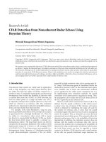
Figure 1: A block diagram for a wireless sensor network tasked for binary hypothesis testing with channel fading statistics.
cases: (1) CSIF: the fusion center has access to the instanta-
neous CSI. (2) NOCSIF: the fusion center does not have ac-
cess to the instantaneous CSI. We note here that for the CSIF
case, the design of sensor decision rules does not require CSI;
the CSI is only used in the fusion rule design, which is rea-
sonable due to the typical generous resource constraint at the
fusion center. Its computation, however, is very involved and
has to resort to exhaustive search. On the other hand, as to be
elaborated, the NOCSIF case can be reduced to the channel
aware design where one averages the channel transition prob-
ability with respect to the fading channel using the known

fading statistics.
We show that the sensor decision rules amount to lo-
cal LRTs for both cases. Compared with the existing channel
aware design based on CSI, the proposed approaches have an
important practical advantage: the sensor decision rules re-
main the same for different CSI, as long as the fading statis-
tics remain unchanged. This enables distributed design as no
global CSI is used in determining the local decision rules. We
also demonstrate through numerical examples that the pro-
posed schemes suffer small performance loss compared with
the CSI-based approach, as long as the CSI is available at the
fusion center, that is, used in the fusion rule design.
The paper is organized as follows. Section 2 describes the
system model and problem formulation. In Section 3,wees-
tablish, for both the CSIF and NOCSIF cases, the optimality
of LRTs at local sensors for minimum average error proba-
bility at the fusion center. Numerical examples are presented
in Section 4 to evaluate the performance of these two cases.
Finally, we conclude in Section 5.
2. STATEMENT OF THE PROBLEM
Consider the problem of testing two hypotheses, denoted by
H
0
and H
1
, with respective prior probabilities π
0
and π
1
.A

total number of K sensors are used to collect observations
X
k
,fork = 1, , K. We assume throughout this paper that
the observations are conditionally independent, that is,
p

X
1
, , X
K
| H
i

=
K

k=1
p

X
k
| H
i

, i = 0, 1. (1)
Without this assumption, the distributed detection design
becomes much more complicated from an algorithmic view-
point [12]. The optimal design is not completely understood
even in the simplest case [13]. Upon observing X

k
,eachlocal
sensor makes a binary decision
1
U
k
= γ
k

X
k

, k = 1, , K. (2)
The decisions U
k
are sent to a fusion center through parallel
transmission channels characterized by
p

Y
1
, , Y
K
| U
1
, , U
K
, g
1
, , g

K

=
K

k=1
p

Y
k
| U
k
, g
k

,
(3)
where g
={g
1
, , g
K
} represents the CSI. Thus, from (3),
the channels are orthogonal to each other, which can be
achieved through, for example, partitioning time, frequency,
or combinations thereof. For the CSIF case, the fusion center
takes both the channel output y
={Y
1
, , Y

K
} and the CSI,
g, and makes a final decision using the optimal fusion rule to
obtain U
0
∈{H
0
, H
1
},
U
0
= γ
0
(y, g). (4)
For the case of NOCSIF, the fusion output depends on the
channel output and the channel fading statistics,
U
0
= γ
0
(y), (5)
where the dependence of fading channel statistics is implicit
in the above expression. An error happens if U
0
differs from
the t rue hypothesis. Thus, the error probability at the fusion
center, conditioned on a given g,is
P
e0


γ
0
, , γ
K
| g

 P
r

U
0
= H | γ
0
, , γ
K
, g

,(6)
where H is the true hypothesis. Our goal is, therefore, to de-
sign the optimal mapping γ
k
(·) for each sensor and the fu-
sion center that minimizes the average error probability, de-
fined as
min
γ
0
(·), ,γ
K

(·)

g
P
e0

γ
0
, , γ
K
| g

p(g)dg,(7)
where p(g) is the distribution of CSI. A simple diagram illus-
trating the model is given in Figure 1.
1
The extension to the case with multibit local decision is straig htforward
by following the same spirit as in [10].
B. Liu and B. Chen 3
We point out here that integrating the transmission
channels into the fusion rule design has been investigated be-
fore [ 14, 15]. The optimal fusion rule in the Bayesian sense
amounts to the maximum a posteriori probability (MAP) de-
cision, that is,
f

Y
1
, , Y
K

| H
1

f

Y
1
, , Y
K
| H
0

>
<
H
1
H
0
π
0
π
1
. (8)
Given specified local sensor signaling schemes and the chan-
nel characterization, this MAP decision rule can be obtained
in a straightforward manner. As such, we will focus on the
local decision r ule design without further elaborating on the
optimal fusion rule design.
3. DESIGN OF OPTIMAL LOCAL DECISION RULES
As in [9, 10], we adopt in the following a person-by-person

optimization (PBPO) approach, that is, we optimize the local
decision rule for the kth sensor given fixed decision rules at
all other sensors and a fixed fusion rule. As such, the condi-
tions obtained are necessary, but not sufficient, for optimal-
ity. Denote
u
=

U
1
, U
2
, , U
K

, x =

X
1
, X
2
, , X
K

,
(9)
the average error probability at the fusion center is
P
e0
=


g
1

i=0
π
i
P

U
0
= 1 − i | H
i
, g

p(g)dg
=

g
1

i=0
π
i

y
P

U
0

= 1 − i | y, g


u
p(y | u, g)
×

x
P(u | x)p

x | H
i

p(g) dx dy dg,
(10)
where, different from the CSI-based channel aware design,
the local decision r ules do not depend on the instantaneous
CSI. Next, we will derive the optimal decision rules by fur-
ther expanding the error probability with respect to the kth
decision rule γ
k
(·) for the two different cases.
3.1. The CSIF case
We first consider the case where the fusion center knows the
instantaneous CSI. Define, for k
= 1, , K and i = 0, 1,
u
k
=


U
1
, , U
k−1
, U
k+1
, , U
K

,
u
ki
=

U
1
, , U
k−1
, U
k
= i, U
k+1
, , U
K

,
y
k
=


Y
1
, , Y
k−1
, Y
k+1
, , Y
K

.
(11)
We can expand the average error probability in (10)withre-
spect to the kth decision rule γ
k
(·), and we get
P
e0
=

X
k
P

U
k
= 1 | X
k

×


π
0
p

X
k
| H
0

A
k
− π
1
p

X
k
| H
1

B
k

dX
k
+ C,
(12)
where
C
=


X
k

1

i=0
π
i
p

X
k
| H
i

×

y

g
P

U
0
= 1 − i | y, g


u
k

p

y | u
k0
, g

×
p(g)p

u
k
| H
i

dg dy

dX
k
(13)
is a constant with regard to U
k
,and
A
k
=

y

g
P


U
0
=1 | y, g



u
k

p

y | u
k1
, g

− p

y | u
k0
, g

×
p(g)P

u
k
| H
0



dg dy,
(14)
B
k
=

y

g
P

U
0
=0 | y, g



u
k

p

y | u
k0
, g

−
p


y | u
k1
, g

×
p(g)P

u
k
| H
1


dg dy.
(15)
To minimize P
e0
, one can see from (12) that the optimal de-
cision rule for the kth sensor is
P

U
k
= 1 | X
k

=
⎧
⎨
⎩

0, π
0
p

X
k
| H
0

A
k
>π
1
p

X
k
| H
1

B
k
,
1, otherwise.
(16)
Let us further take a look at A
k
in (14). We can rewrite it as
A
k

=

y
k

P

U
0
= 1 | y
k
, U
k
= 1

−
P

U
0
= 1 | y
k
, U
k
= 0

p

y
k

| H
0

dy
k
.
(17)
Then, as shown in Appendix A, A
k
> 0aslongas
L

U
k


P

U
k
| H
1

P

U
k
| H
0


(18)
is a monotone increasing function of U
k
(monotone LR in-
dex assignment), that is,
L

U
k
= 1

>L

U
k
= 0

. (19)
Similarly, B
k
> 0 if condition (19) is satisfied. This immedi-
ately leads to the following result.
Theorem 1. For the distributed detection problem with un-
known CSI only at local sensors, the optimal local decision rule
for the kth sens or amounts to the following LRT assuming con-
dition (19) is satisfied,
P

U
k

= 1 | X
k

=
⎧
⎪
⎪
⎪
⎪
⎨
⎪
⎪
⎪
⎪
⎩
1,
p

X
k
| H
1

p

X
k
| H
0


≥
π
0
A
k
π
1
B
k
,
0,
p

X
k
| H
1

p

X
k
| H
0

<
π
0
A
k

π
1
B
k
,
(20)
where A
k
and B
k
are defined in (14) and (15),respectively.
4 EURASIP Journal on Wireless Communications and Networking
An alternative derivation, along the line of [11], is given
in Appendix B.
Although the optimal local decision rule for each local
sensor is explicitly formulated in (20), it is not amenable to
direct numerical evaluation: in (14)and(15), the integrand
involves the fusion rule that is a highly nonlinear function of
the CSI g, making the integration formidable. The only pos-
sible way of finding the optimal local decision rules appears
to be an exhaustive search, whose complexity becomes pro-
hibitive when K is large.
This numerical challenge motivates an alternative ap-
proach: instead of minimizing the average error probability,
one can first marginalize the channel transition probability
followed by the application of standard channel aware design
[8–10]. That is, we first compute p(y
| u) by marginalizing
out the channel g using the channel fading statistics:
p(y

| u) =

g
p(y | u, g)p(g)dg. (21)
With this marginalization, we can use the channel aware de-
sign approach [ 9] that tends to the “averaged” transmission
channel. The difference between this alternative approach
and that of minimizing (7) is in the way that the channel
fading statistics, p(g), is utilized. In using (7), the variable
to be averaged is P
e0
(γ
0
, , γ
K
| g), which is a highly non-
linear function of the decision rules, whereas the alterna-
tive approach uses p(g) to obtain the marginalized channel
transition probability, thus enabling the direct application
of the channel aware approach. This difference can also be
explained using Figure 1. The alternative approach averages
each transmission channel over respective channel statistics
g
i
to obtain p(Y
i
| U
i
), while the CSIF case averages all the
transmission channels and the fusion center (the part in the

dashed box in Figure 1) over channel statistics g to obtain
P

U
0
| u

=

g

y
P

U
0
| y, g

p

y | u, g

p(g)dy dg. (22)
It turns out that this alternative approach is a direct conse-
quence of the NOCSIF, as elaborated below.
3.2. The NOCSIF case
Here we consider the case where the fusion center does not
know the instantaneous CSI. Therefore, we have
P


U
0
= 1 − i | y, g

=
P

U
0
= 1 − i | y

. (23)
As the fusion rule no longer depends on g, the average error
probability in (10)canberewrittenas
P
e0
=
1

i=0
π
i

y

u
P

U
0

= 1 − i | y



g
p

y | u, g

p(g)dg

×

x
P

u | x

p

x | H
i

dx dy,
(24)
where integration with respect to g is carried out first. Notice
that the term (

g
p(y | u, g)p(g)dg) precisely describes the

marginalized transmission channels (cf. (21)). This leads to
the standard channel aware design where the transmission
channels are chara cterized by p(y
| u). From [9], we have a
result resembling that of Theorem 1 except that A
k
, B
k
,and
C are replaced by A

k
, B

k
,andC

,
A

k
=

y
P

U
0
= 1 | y




u
k

p

y | u
k1

−
p

y | u
k0

×
P

u
k
| H
0


dy,
B

k
=


y
P

U
0
= 0 | y



u
k

p

y | u
k0

−
p

y | u
k1

×
P

u
k
| H

1


dy,
C

=

X
k

1

i=0
π
i
p

X
k
| H
i


y
P

U
0
=1 −i | y



u
k
p

y | u
k0

×
p

u
k
| H
i

dy

dX
k
.
(25)
Contrary to the CSIF case, A

k
, B

k
for the NOCSIF case are

much easier to evaluate.
4. PERFORMANCE EVALUATION
In this section, we first use a two-sensor example to eval-
uate the performance of both the CSIF and NOCSIF cases
and compare them with the clairvoyant case where the global
channel information is known to the designer. For conve-
nience, we call the clairvoyant case the CSI case. Consider the
detection of a known signal S in zero-mean complex Gaus-
sian noises that are independent and identically distributed
(i.i.d.) for the two sensors, that is, for k
= 1, 2,
H
0
: X
k
= N
k
, H
1
: X
k
= S + N
k
,
(26)
with N
1
and N
2
being i.i.d. CN (0, σ

2
1
). Without loss of gen-
erality, we assume S
= 1andσ
2
1
= 2.
Each sensor makes a binary decision based on its obser-
vation X
k
,
U
k
= γ
k

X
k

, U
k
∈{0, 1}, (27)
and then transmits it through a Rayleigh fading channel to
the fusion center. Notice that U
k
∈{0, 1} implies an on-off
signaling, thus enabling the detection at the fusion center in
the absence of CSI (i.e., the NOCSIF case). The channel out-
put is

Y
k
= g
k
U
k
+ W
k
, (28)
where g
1
, g
2
are independently distributed with zero-mean
complex Gaussian distributions CN (0, σ
2
g
1
)andCN (0, σ
2
g
2
),
B. Liu and B. Chen 5
10864202
Signal-to-noise ratio (dB)
0.3
0.32
0.34
0.36

0.38
0.4
0.42
0.44
0.46
Average error probability
CSI
CSIF
CSIF 1
NOCSI
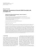
Figure 2: Average error probability versus channel SNR for identi-
cal channel distribution.
respectively. W
1
, W
2
are i.i.d. zero-mean complex Gaussian
noises with distribution CN (0, σ
2
2
).
We first consider a symmetric case where the CSI is iden-
tically distributed, that is, σ
g
2
1
= σ
g
2
2

. Without loss of gen-
erality, we assume σ
g
2
1
= σ
g
2
2
= 1. In Figure 2, with the as-
sumption of equal prior probability, the average error prob-
abilities as a function of the average signal-to-noise ratio
(SNR) of the received signal at the fusion center are plot-
ted for the CSIF and NOCSIF cases, along with the CSI case.
We also plot a curve, legended with “CSIF1” in Figure 2,
where the local sensors use thresholds obtained via the NOC-
SIF approach but the fusion center implements a fusion rule
that utilizes the CSI g. The motivation is twofold. First,
estimating g at the fusion center is typically feasible. Sec-
ond and more importantly, the threshold design for NOC-
SIF is much simpler compared with CSIF, as explained in
Section 3.1.
In evaluating the performance of CSIF case, we consider
the following two methods to get the optimal thresholds for
local sensors.
Exhaustive search method
We first partition the space of likelihood ratio of observations
into many smal l disjoint cells. For each cell, we compute the
average error probability at the fusion center by using the
center point of the cell (for small enough cell size, the cen-

ter point can be considered “representive” of the whole cell)
as the local thresholds. After evaluating the performance for
all the cells, we choose the one with smallest average error
probability as our optimal thresholds. Intuitively, one can get
arbitrarily close to the optimal thresholds by decreasing the
cell size, which proportionally increases the computational
complexity.
Greedy search
(1) choose initial thresholds t
(0)
, for example, the thresh-
olds obtained via the NOCSIF case and set r
= 0(iter-
ation index);
(2) compute the average error probability using t
(0)
as lo-
cal thresholds;
(3) choose several directions. For example, for two-sensor
case, we can choose (1, 0), (
−1, 0), (0, 1), and (0, −1)
as our directions;
(4) choose a small stepsize
;
(5) move the current thresholds t
(r)
one stepsize along
each direction and compute the average error proba-
bility using the new thresholds;
(6) compare the error probability of using current thresh-

olds t
(r)
and new thresholds and assign the thresholds
corresponding to the smallest one as t
(r+1)
;
(7) if t
(r+1)
= t
(r)
, stop; otherwise, set r = r +1andgoto
step (5).
Greedy search method is much faster than exhaustive
search method since we do not need to compute the aver-
age error probability corresponding to every point. But it can
only guarantee convergence to a local minimum point.
As seen from Figure 2, the CSI case has the best perfor-
mance and NOCSIF case has the worst perfor mance. This
is true because the designer has the most information in
the clairvoyant case and the least information in NOCSIF
case. The CSIF case is only slightly worse than the CSI
case but is much better than the NO CSIF case. The dif-
ference of CSIF1 and CSIF is almost indistinguishable. The
explanation is that the performance is much more sensi-
tive to the fusion rule than to the local sensor thresholds.
This phenomenon has been observed before: the error prob-
ability versus threshold plot is r a ther flat near the opti-
mum point, hence is robust to small changes in thresh-
olds.
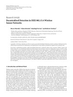
We also consider an asymmetric case where σ

g
2
1
= σ
g
2
2
.
As plotted in Figure 3 where σ
g
2
1
= 1andσ
g
2
2
= 3, all three
cases with known CSI at the fusion center have similar per-
formance and are much better than the NOCSIF case. This is
consistent with the symmetric case.
As we stated above, for the system with only two lo-
cal sensors, a mixed approach (CSIF1) achieves almost same
performance to that of the CSIF case. In the following, we
show that the same holds true even in the large system
regime, that is, as K increasing. We first consider the Bayesian
framework. As K goes to infinity, all the local sensors use the
same local decision rule [16] and the optimal local thresholds
are determined by maximizing the Chernoff information to
achieve the best error exponent,
C


p

Y | H
0

, p

Y | H
1

=−
min
0≤s≤1
log


p

Y | H
0

s
p

Y | H
1

1−s
dY


.
(29)
For simplicity, we consider another performance measure,
Bhattacharyya’s distance, which is an approximation of
6 EURASIP Journal on Wireless Communications and Networking
10864202
Signal-to-noise ratio (dB)
0.3
0.32
0.34
0.36
0.38
0.4
0.42
Average error probability
CSI
CSIF
CSIF 1
NOCSI
Figure 3: Average error probability versus channel SNR for non-
identical channel distribution.
21.510.500.511.52
Local threshold
0
0.002
0.004
0.006
0.008
0.01

0.012
0.014
Bhattacharyya distance
NOCSIF
CSIF
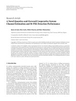
Figure 4: Bhattacharyya’s distance versus the local threshold at the
local sensors.
Chernoff information by setting s = 1/2,
B

p

Y | H
0

, p

Y | H
1

=−
log


p

Y | H
0

1/2

p

Y | H
1

1/2
dY

=−
log



p

Y | H
0

p

Y | H
1


1/2
p

Y | H
1


dY

.
(30)
From Figure 4, which g ives Bhattachar yya’s distance as a
function of local threshold for both CSIF and NOCSIF cases
21.510.500.511.52
Local threshold
0
0.01
0.02
0.03
0.04
0.05
0.06
KL distance
NOCSIF
CSIF
Figure 5: KL distance versus the local threshold at the local sensors.
with σ
2
2
= 2andσ
2
g
= 1, we can observe that the optimal
threshold obtained in NOCSIF case is close to that of the
CSIF case.
Alternatively, under the Neyman-Pearson framework,
the Kullack-Leibler (KL) distance gives the asymptotic error

exponent,
KL

p

Y | H
0

, p

Y | H
1

=
E
H
0

log

p

Y | H
0

p

Y | H
1



=

p

Y | H
0

log

p

Y | H
0

p

Y | H
1


dY.
(31)
In Figure 5, with the same setting as in Figure 4, the KL dis-
tance as a function of local threshold for both CSIF and
NOCSIF cases is plotted and we can also observe that the op-
timal local thresholds obtained in NOCSIF and CSIF cases
are close to each other.
5. CONCLUSIONS
In this paper we investigated the design of the distributed

detection problem with only channel fading statistics avail-
able to the designer. Restricted to conditional independent
observations and binary local sensor decisions, we derive the
necessary conditions for optimal local sensor decision rules
that minimize the average error probability for the CSIF and
NOCSIF cases. Numerical results indicate that a mixed ap-
proach where the sensors use the decision rules from the
NOCSIF approach w hile the fusion center implements a fu-
sion rule using the CSI achieves almost identical perfor-
mance to that of the CSIF case.
B. Liu and B. Chen 7
APPENDICES
A. PROOF OF A
K
> 0 AND B
K
> 0
P

H
1
| y
k
, U
k

=
p

H

1
, y
k
, U
k

p

y
k
, U
k

=
p

y
k
, U
k
| H
1

P

H
1

p


y
k
, U
k
| H
0

P

H
0

+ p

y
k
, U
k
| H
1

P

H
1

=
π
1
p


y
k
| U
k
, H
1

P

U
k
| H
1

π
0
p

y
k
| U
k
, H
0

P

U
k

| H
0

+π
1
p

y
k
| U
k
, H
1

P

U
k
| H
1

.
(A.1)
Since the observ ations, X
1
, , X
K
, are conditionally inde-
pendent and the local decision in each sensor depends only
on its own observation, the local decisions are also condi-

tionally independent for a given hypothesis. In addition, the
local decisions are transmitted through orthogonal channels,
thus the channel output for one sensor is conditionally in-
dependent to the channel input from a nother sensor. There-
fore,
p

y
k
| U
k
, H
1

=
p

y
k
| H
1

. (A.2)
Defining the likelihood ratio function for the local decision
at the kth sensor,
L

U
k



P

U
k
| H
1

P

U
k
| H
0

. (A.3)
Then
P

H
1
| y
k
, U
k

=
π
1
p


y
k
| H
1

P

U
k
| H
1

π
0
p

y
k
| H
0

P

U
k
| H
0

+ π

1
p

y
k
| H
1

P

U
k
| H
1

=
π
1
p

y
k
| H
1

L

U
k


π
0
p

y
k
| H
0

+ π
1
p

y
k
| H
1

L

U
k

(A.4)
which is a monotone increasing function of L(U
k
). Then,
given a monotone LR index assignment for the local output,
that is, L(U
k

= 1) >L(U
k
= 0), P(H
1
| y
k
, U
k
) is a monotone
increasing function of U
k
.Thus,
P

H
1
| y
k
, U
k
= 0

<P

H
1
| y
k
, U
k

= 1

. (A.5)
Similarly, we can get
P

H
0
| y
k
, U
k
= 0

>P

H
0
| y
k
, U
k
= 1

. (A.6)
The optimum fusion rule is a maximum a posteriori rule
(i.e., to minimize error probability). Thus deciding U
0
= 1
for a given y

k
and U
k
= 0requires
P

H
1
| y
k
, U
k
= 0

>P

H
0
| y
k
, U
k
= 0

. (A.7)
From (A.5)and(A.6), (A.7)implies
P

H
1

| y
k
, U
k
= 1

>P

H
0
| y
k
, U
k
= 1

. (A.8)
Therefore, we must have U
0
= 1 for the same y
k
with U
k
= 1.
Thus
P

U
0
= 1 | y

k
, U
k
= 0

<P

U
0
= 1 | y
k
, U
k
= 1

(A.9)
and further,
A
k
> 0. (A.10)
Similarly, one can show
P

U
0
= 0 | y
k
, U
k
= 0


>P

U
0
= 0 | y
k
, U
k
= 1

(A.11)
and further,
B
k
> 0. (A.12)
B. ALTERNATIVE DERIVATION FOR OPTIMAL
LOCAL DECISION RULES
From [7, Proposition 2.2], with a cost function F :
{0, 1}×
Z ×{H
0
, H
1
}→R and a random variable z which takes
values in the set Z and is independent of X conditioned on
any hypothesis, the optimal decision r ule that minimizes the
cost E[F(γ(X), z, H)] is
γ(X)
= arg min

U=0,1
1

j=0
P

H
j
| X

α

H
j
, U

,(B.1)
where
α

H
j
, d

=
E

F

U, z, H

j

|
H
j

. (B.2)
Assuming the cost that we want to minimize at the fusion
center can be written as
J
= E

C

γ
0
(y, g), u, H

(B.3)
and we further have
J
= E

C

γ
0
(y, g), u, H

=

E

C

γ
0

Y
k
, y
k
, g
k
, g
k

, γ
k

X
k

, u
k
, H

=
E

E


C

γ
0

Y
k
, y
k
, g
k
, g
k

, γ
k

X
k

, u
k
, H

|
u
k
, y
k

, g
k
, g
k
, X
k
, H

=
E

E

C

γ
0

Y
k
, y
k
, g
k
, g
k

, γ
k


X
k

, u
k
, H

|
X
k
, g
k

=
E


Y
k
C

γ
0

Y
k
, y
k
, g
k

, g
k

, γ
k

X
k

, u
k
, H

×
p

Y
k
| γ
k

X
k

, g
k

dY
k


,
(B.4)
where g
k
= [g
1
, , g
k−1
, g
k+1
, g
K
]and(B.4) follows that con-
ditioned on γ
k
(X
k
)andg
k
, the channel output Y
k
is indepen-
dent of everything else.
8 EURASIP Journal on Wireless Communications and Networking
Defining X = X
k
, z = (y
k
, u
k

, g),
F

U
k
, z, H

=

Y
k
C

γ
0

Y
k
, y
k
, g

, U
k
, u
k
, H

p


Y
k
| U
k
, g
k

dY
k
(B.5)
and substituting them into (B.1), we obtain the optimal local
decision rule for kth sensor:
γ
k

X
k

=
arg min
U
k
=0,1
1

j=0
P

H
j

| X
k

α
k

H
j
, U
k

,(B.6)
where
α
k

H
j
, U
k

=
E


Y
k
C

γ

0

Y
k
, y
k
, g

, U
k
, u
k
, H
j

p

Y
k
| U
k
, g
k

dY
k
| H
j

.

(B.7)
Since
P

H
j
| X
k

=
p

X
k
| H
j

π
j

1
i
=0
p

X
k
| H
i


π
i
,(B.8)
(B.6)isequivalentto
γ
k

X
k

= arg min
U
k
=0,1
1

j=0
π
j
p

X
k
| H
j

α
k

H

j
, U
k

=
arg min
U
k
=0,1
1

j=0
p

X
k
| H
j

b
k

H
j
, U
k

,
(B.9)
where

b
k

H
j
, U
k

= π
j
α
k

H
j
, U
k

. (B.10)
Thus, the optimal local decision rule for the kth sensor is
γ
k

X
k

=
⎧
⎪
⎪

⎪
⎪
⎨
⎪
⎪
⎪
⎪
⎩
0, P

X
k
| H
0

b
k

H
0
,1

−
b
k

H
0
,0


≥
P

X
k
| H
1

b
k

H
1
,0

−
b
k

H
1
,1

,
1, otherwise.
(B.11)
In the approach proposed in this paper, the objective is to
minimize the average error probability at the fusion center,
J
=


g
P

γ
0
(y, g) = H

p(g) dg. (B.12)
Thus we have
α
k

H
j
, U
k

=

y

g
P

U
0
= 1 − j | y, g

×



u
k
p

y | u
k
, U
k
, g

p(g)P

u
k
| H
j


dg dy.
(B.13)
It is straightforward to see that (α
k
(H
0
,1) − α
k
(H
0

,0)) is
the same as A
k
in (14)and(α
k
(H
1
,0) − α
k
(H
1
, 1)) is the
same as B
k
in (15). Therefore, (B.11)isequivalentto(20)
in Theorem 1.
ACKNOWLEDGMENT
This work was supported in part by the National Science
Foundation under Grant 0501534.
REFERENCES
[1] R. Radner, “Team decision problems,” Annals of Mathematical
Statistics, vol. 33, no. 3, pp. 857–881, 1962.
[2] R. R. Tenney and N. R. Sandell Jr., “Detection with distributed
sensors,” IEEE Transactions on Aerospace and Electronic Sys-
tems, vol. 17, no. 4, pp. 501–510, 1981.
[3] P. K. Varshney, Distr ibuted Detection and Data Fusion,
Springer, New York, NY, USA, 1997.
[4] A. R. Reibman and L. W. Nolte, “Optimal detection and per-
formance of distributed sensor systems,” IEEE Transactions on
Aerospace and Electronic Systems, vol. 23, no. 1, pp. 24–30,

1987.
[5] I. Y. Hoballah and P. K. Varshney, “Distributed Bayesian signal
detection,” IEEE Transactions on Information Theory, vol. 35,
no. 5, pp. 995–1000, 1989.
[6] S. C. A. Thomopoulos, R. Viswanathan, and D. K. Bougou-
lias, “Optimal distributed decision fusion,” IEEE Transactions
on Aerospace and Electronic Systems, vol. 25, no. 5, pp. 761–765,
1989.
[7] J. N. Tsitsiklis, “Decentralized detection,” in Advances in Sta-
tistical Signal Processing,H.V.PoorandJ.B.Thomas,Eds.,pp.
297–344, JAI Press, Greenwich, Conn, USA, 1993.
[8] T. M. Duman and M. Salehi, “Decentralized detection over
multiple-access channels,” IEEE Transactions on Aerospace and
Electronic Systems, vol. 34, no. 2, pp. 469–476, 1998.
[9] B. Chen and P. K. Willett, “On the optimality of the likelihood-
ratio test for local sensor decision rules in the presence of
nonideal channels,” IEEE Transactions on Information Theory,
vol. 51, no. 2, pp. 693–699, 2005.
[10] B. Liu and B. Chen, “Channel-optimized quantizers for de-
centralized detection in sensor networks,” IEEE Transactions
on Information Theory, vol. 52, no. 7, pp. 3349–3358, 2006.
[11] A. Kashyap, “Comments on “on the optimality of the
likelihood-ratio test for local sensor decision rules in the pres-
ence of nonideal channels”,” IEEE Transactions on Informat ion
Theory, vol. 52, no. 3, pp. 1274–1275, 2006.
[12] J. N. Tsitsiklis and M. Athans, “On the complexity of decen-
tralized decision making and detection problems,” IEEE Trans-
actions on Automatic Control, vol. 30, no. 5, pp. 440–446, 1985.
[13] P. K. Willett, P. F. Swaszek, and R. S. Blum, “The good, bad,
and ugly : distributed detection of a known signal in dependent

gaussian noise,” IEEE Transactions on Signal Processing, vol. 48,
no. 12, pp. 3266–3279, 2000.
[14] B. Chen, R. Jiang, T. Kasetkasem, and P. K. Varshney, “Fusion
of decisions transmitted over fading channels in wireless sen-
sor networks,” in Proceedings of the 36th Asilomar Conference
on Signals, Systems and Computers, vol. 2, pp. 1184–1188, Pa-
cific Grove, Calif, USA, November 2002.
[15] R. Niu, B. Chen, and P. K. Varshney, “Decision fusion rules
in wireless sensor networks using fading channel statistics,”
in Proceedings of the 37th Annual Conference on Information
Sciences and Systems (CISS ’03),Baltimore,Md,USA,March
2003.
[16] J. N. Tsitsiklis, “Extremal properties of likelihood-ratio quan-
tizers,” IEEE Transactions on Communications,vol.41,no.4,
pp. 550–558, 1993.