Báo cáo hóa học: " REDUCING THE NUMBER OF FIXED POINTS OF SOME HOMEOMORPHISMS ON NONPRIME 3-MANIFOLDS" ppt
Bạn đang xem bản rút gọn của tài liệu. Xem và tải ngay bản đầy đủ của tài liệu tại đây (764.78 KB, 19 trang )
REDUCING THE NUMBER OF FIXED POINTS OF SOME
HOMEOMORPHISMS ON NONPRIME 3-MANIFOLDS
XUEZHI ZHAO
Received 5 September 2004; Revised 15 March 2005; Accepted 21 July 2005
We will consider the number of fixed points of homeomorphisms composed of finitely
many slide homeomorphisms on closed oriented nonprime 3-manifolds. By isotoping
such homeomorphisms, we try to reduce their fixed point numbers. The numbers ob-
tained are determined by the intersection information of sliding spheres and sliding paths
of the slide homeomorphisms involved.
Copyright © 2006 Xuezhi Zhao. This is an open access article distributed under the Cre-
ative Commons Attribution License, which permits unrestricted use, distribution, and
reproduction in any medium, provided the original work is properly cited.
1. Introduction
Nielsen fixed point theory (see [1, 4]) deals with the estimation of the number of fixed
points of maps in the homotopy class of any given map f : X
→ X. The Nielsen number
N( f ) provides a lower bound. A classical result in Nielsen fixed point theor y is: any map
f : X
→ X is homotopic to a map with exactly N( f ) fixed points if the compact polyhe-
dron X has no local cut point and is not a 2-manifold. This includes all smooth manifolds
with dimension g reater than 2.
It is also an interesting question whether the Nielsen number can be realized as the
number of fixed points of a homeomorphism in the isotopy class of a given homeomor-
phism. In fact, it is just what J. Nielsen expected when he introduced the invariant N( f ).
Assume that X is a closed manifold. The answer to this question is obviously positive
for the unique closed 1-manifold. A positive answer was given by Jiang and Guo [5]for
2-manifolds, and was given by Kelly [7] for manifolds of dimension at least 5.
In [6], Jiang, Wang and Wu proved that for any closed oriented 3-manifold X which
is either Haken or geometric, any orientation-preserving homeomorphism f : X
→ X is
isotopic to a homeomorphism with N( f ) fixed points ([6, Theorem 9.1]). If Thurston’s
geometric conjecture is true, all nonprime 3-manifolds are of this type.
In this paper, we will consider a certain class of homeomorphisms of closed, oriented
3-manifolds that have a connected sum decomposition into prime factors, namely irre-
ducible manifolds and copies of S
2
× S
1
, and at least two factors (nonprime manifolds).
Hindawi Publishing Corporation
Fixed Point Theory and Applications
Volume 2006, Article ID 25897, Pages 1–19
DOI 10.1155/FPTA/2006/25897
2 Fixed points of slide homeomorphisms
It is known from work of Kneser and Milnor that in the oriented setting, the pr ime and
irreducible factors of the decomposition are unique. We examine homeomorphisms that
can be expressed as the composition of finitely many slide homeomorphisms. A so-called
slide homeomorphism is the identity away from a certain stratified open neighborhood,
the sliding set, of a torus, and is defined by a family of rotation-like transformations on
this set. According to McCullough’s result (see [8]), an arbitrary homeomorphism of a re-
ducible 3-manifold can be expressed as the composition of homeomorphisms that comes
in four types, one of which is that of slide homeomorphisms.
In [9], the author considered the Nielsen numbers and fixed points of homeomor-
phisms which are compositions of m slide homeomorphisms on nonprime 3-manifolds.
The fixed point index of the complement of the union of the sliding sets was proved to be
zero. When m
= 2, we found presentations that are in some sense “standard,” for which
the fixed point numbers, the fixed point class coordinates and the fixed point indices for
all fixed points can be determined. Thus, we were able to give some estimating b ounds on
the Nielsen numbers of such kinds of homeomorphisms. The present paper is a continu-
ation of [9]. We will generalize the results for m
= 2 there to the case where m can be an
arbitr ary positive integer. We will focus on a geometrical method to reduce the number of
fixed points in any given isotopy class of such a homeomorphism. The lower bound prop-
erty of Nielsen number implies that our number of fixed points yields an upper bound
for Nielsen number.
The remaining sections are organized as follows. In Section 2, we will fix notation
which will be used throughout this paper, and recall the definition of slide homeomor-
phism. In Section 3, we will show (Lemma 3.4) that away from the sliding set, f can be
isotoped to a fixed point free homeomorphism by an arbitrary small isotopy. Although
each component of this set has zero fixed point index ([9, Theorem 3.2]), the result
here is not very obvious because we are considering fixed points up to isotopy rather
than homotopy. In Section 4, fixed points over the sliding set are considered. It is ar-
gued that f is isotopic to a homeomorphism with finitely many fixed points, and that
the size of this fixed point set is expressible in terms self-intersection data for the slid-
ing set (Proposition 4.6). Reducing the number of fixed points for homeomorphisms in
the isotopy class of f then involves controlling in some sense the number of self inter-
sections; our main result (Theorem 4.11) gives a lower bound for this number. Finally, a
short Section 5 shows that in some cases, one may simplify and “optimize” the sliding set
so that the bound in Section 4 can be further lowered, that is, the number of fixed points
can be further reduced.
2. Conventions and notations
In this section, we will make necessar y conventions in notation, which will be used in
later sections.
(1) The underlying manifold M. In this paper, the manifold M is assumed to b e a closed
oriented 3-manifold, which is nonprime. It is known that M can be written as a connected
sum of finitely many prime 3-manifolds, that is, M
= M
1
#M
2
#···#M
n
#···#M
n
+n
,in
which M
i
is irreducible for 1 ≤ i ≤ n
and M
i
= S
2
× S
1
for n
+1≤ i ≤ n
+ n
. The non-
prime property implies that n
+ n
> 1.
Xuezhi Zhao 3
Take a 3-s phe re and re move n
+2n
open discs to obtain a punctured 3-cell W with
n
+2n
boundary components. We then have that M = W ∪ (∪
n
+n
i=1
M
i
), where M
i
=
M
i
− Int(D
i
)for1≤ i ≤ n
and M
i
= S
2
× I for n
+1≤ i ≤ n
+ n
(see [8]). Each M
i
admits the orientation coincident with that of M, and each ∂M
i
inherits the orientation
of M
i
.
(2) Slide homeomorphisms.LetS be an oriented essential 2-sphere in M, which is
orientation-preservingly isotopic to a boundary component of ∂M
j
.Letα : I → M be
a path without self intersection in M such that α
∩ M
j
= α ∩ S ={α(0),α(1)}.Taketwo
regular neighborhoods N
and N
(N
⊂ Int(N
)) of α ∪ S in M.ThenInt(N
− N
)has
two components which are homeomorphic to S
2
× (0,1) and T
2
× (0,1) respectively. We
write the latter as T(S,α).
Pick a coordinate function c : T(S,α)
→ T
2
× (0,1), where the points in T
2
× (0,1) are
labeled by (θ,ϕ,t), such that the θ-line, c
−1
(θ,∗,∗), is parallel to the oriented path α and
the t-line c
−1
(∗,∗,t) m oves radially away from the path α when the value of t is increased.
A slide homeomorphism s : M
→ M determined by α and S is defined by
s(x)
=
⎧
⎨
⎩
c
−1
(θ +2πt,ϕ,t)ifx = c
−1
(θ,ϕ,t) ∈ T(S,α),
x otherwise,
(2.1)
denoted by s(S,α). The sets T(S,α), S and α are said to be respectively the sliding set,
sliding sphere and sliding path of s(S,α).
(3) Orientations and isotopies. Since all manifolds under consideration are oriented,
including sliding spheres and sliding paths, isotopies here are considered to be ambient
and orientation-preserving. For example, if M
= M
1
#M
2
isaconnectedsumoftwoprime
manifolds, ∂M
1
and ∂M
2
are not regarded as isotopic.
(4) Fundamental groups and path classes. Consider the construction M
=W∪(∪
n
+n
i=1
M
i
)
of M.Wechooseapointx
0
in W as its base point. To any path γ with ending points in W
there corresponds uniquely an element
γ
∗
γγ
−1
∗∗
in π
1
(M,x
0
), where γ
∗
and γ
∗∗
are path
from x
0
to γ(0) and γ(1) in W respectively. By abuse of notation, we write it simply as
γ.Choosex
j
∈ ∂M
j
as base point of M
j
for j = 1,2, ,n
+ n
.Thus,eachπ
1
(M
j
,x
j
)is
embedded into π
1
(M,x
0
) in a natural way as above, and hence π
1
(M,x
0
)isthefreeprod-
uct of π
1
(M
j
,x
j
), j = 1,2, ,n
+ n
. We write simply as π
1
(M,x
0
) = π
1
(M
1
) ∗ π
1
(M
2
) ∗
···∗
π
1
(M
n
+n
), which is also equal to π
1
(M
1
) ∗ π
1
(M
2
) ∗···∗π
1
(M
n
+n
).
(5) The homeomorphism f .Fromnowon, f is assumed to be a homeomorphism com-
posed of finitely many slide homeomorphisms, that is, f
= s(S
m
,α
m
) ◦ s(S
m−1
,α
m−1
) ◦
···◦
s(S
1
,α
1
). The union ∪
m
j
=1
T(S
j
,α
j
) of all sliding sets is said to the sliding set of f .For
a simplification in notation, we write s
m
···m
for the composition s(S
m
,α
m
) ◦ s(S
m
−1
,
α
m
−1
) ◦···◦s(S
m
,α
m
)foranym
and m
(1 ≤ m
<m
≤ m). In particular, s(S
j
,α
j
)is
simply written as s
j
.
(6) General position. Consider the slide homeomorphisms whose composition is f .We
can ensure the sliding paths α
1
,α
2
, ,α
m
, a nd sliding spheres S
1
,S
2
, ,S
m
areingeneral
position relative to the set
∪
m
j
=1
{α
j
(0),α
j
(1)}. Thus, these sliding paths have no intersec-
tion, and α
i
intersects with S
j
transversally for i = j. Since each sliding sphere is isotopic
to a component of
−∂W, we can arrange these sliding spheres to be disjoint. In this sit-
uation, if each sliding set T(S
j
,α
j
) is in a small neig hborhood of α
j
∪ S
j
,thenumber
4 Fixed points of slide homeomorphisms
α
i
q
(i,j;1)
q
(i,j;2)
S
j
······
Figure 2.1
of components of intersection of two sliding sets T(S
j
,α
j
)andT(S
j
,α
j
) is equal to
the number of points in (α
j
∪ S
j
) ∩ (α
j
∪ S
j
)forall j
and j
with j
= j
. In this
situation, we say that the sliding set
∪
m
j
=1
T(S
j
,α
j
)of f is in general position.
(7) Components B
(∗,∗;∗)
of the intersection of sliding sets. If the sliding set ∪
m
j
=1
T(S
j
,α
j
)
is in general position, the points in α
i
∩ S
j
(i = j) are denoted by q
(i, j;1)
,q
(i, j;2)
, ,
q
(i, j;|α
i
∩S
j
|)
(see Figure 2.1), where the last subscript indicates the order in α
i
∩ S
j
along
the direction of α
i
, that is, α
−1
i
(q
(i, j;k
)
) <α
−1
i
(q
(i, j;k
)
)inI = [0,1]ifandonlyifk
<
k
. The corresponding components of T(S
i
,α
i
) ∩ T(S
j
,α
j
) nearby are written as B
(i, j;1)
,
B
(i, j;2)
, ,B
(i, j;|α
i
∩S
j
|)
.Obviously,wehave
Proposition 2.1. If the sliding set
∪
m
j
=1
T(S
j
,α
j
) is in general position, then each B
(∗,∗;∗)
is
homeomorphic to a solid torus, and T(S
i
,α
i
) ∩ T(S
j
,α
j
) = (
|α
i
∩S
j
|
k=1
B
(i, j;k)
) (
|α
j
∩S
i
|
l=1
B
(j,i;l)
)
for any i and j,wherei, j
= 1,2, ,m with i = j.
3. Removing fixed points on the complement of sliding set
Consider our homeomorphism f . Since the fixed point set of each slide homeomorphsim
s
i
is just M − T(S
i
,α
i
), the points in the complement M −∪
m
j
=1
T(S
j
,α
j
) of the sliding set
of f are totally contained in the fixed p oint set of f .In[9], we proved that this isolated
fixed point set has zero fixed point index. In this section, we will show that this fixed point
set can be removed by arbitrary small isotopy.
The following definition is originally from [2].
Definit ion 3.1. Let Γ : N
→ TN be a vector field on a compact smooth n-manifold N.
The manifold N is said to be a manifold with corners for the vector field Γ if Γ has no
singular points on ∂N and if ∂N can be considered a union of (n
− 1)-manifolds (with
boundaries) ∂
o
N, ∂
+
N and ∂
−
N with ∂
+
N ∩ ∂
−
N =∅such that Γ(x)istangentto∂
o
N
for x
∈ ∂
o
N, points inward to N for x ∈ ∂
−
N and points outward from N for x ∈ ∂
+
N.
Clearly, for an n-manifold N with corners, both of ∂
+
N ∩ ∂
o
N and ∂
−
N ∩ ∂
o
N are
(n
− 2)-dimensional closed manifolds. A simple example is the following.
Xuezhi Zhao 5
Example 3.2. A constant vector field on R
2
is given by Γ(x, y) = (1, 0). Then the subset
N
= [0,1] × [0,1] is a manifold with corners for such a vector field Γ,with∂
o
N = [0,1] ×
{
0,1}, ∂
−
N ={0}×[0,1] and ∂
+
N ={1}×[0,1].
The next lemma is a kind of generalization of the Poincar
´
e-Hopf vector field index
theorem. There are some similar statements in dynamical system theory, see for example
[3, Lemma A.1.3].
Lemma 3.3. Let N be a 3-manifold with corners for a vector field Γ.Iftheboundary∂N is
a disjoint union of m-copies of a sphere such that ∂
o
N is a disjoint union of m-copies of an
annulus, and either ∂
+
N or ∂
−
N is a disjoint union of m-copies of a disc, then we can change
Γ relative to a neighborhood of ∂N in N into a nonsingular vector field Γ
.
Proof. Through a coordinate function, each component of ∂N canberegardedasoneof
the following:
C
k
=
(x, y,z):|x|≤4, (y − 8k)
2
+ z
2
= 4orx =±4, (y − 8k)
2
+ z
2
≤ 4
, (3.1)
where k
= 1,2, ,m.Since∂
+
N ∩ ∂
−
N =∅, we may assume that
∂
o
N =∪
m
k
=1
(x, y,z):|x|≤4, (y − 8k)
2
+ z
2
= 4
,
∂
−
N =∪
m
k
=1
(x, y,z):x = 4, (y − 8k)
2
+ z
2
≤ 4
,
∂
+
N =∪
m
k
=1
(x, y,z):x =−4, (y − 8k)
2
+ z
2
≤ 4
.
(3.2)
Regard a neighborhood of ∂N as a subset outside of the cylinders:
D
k
=
(x, y,z):|x|≤4, (y − 8k)
2
+ z
2
≤ 4
, k = 1,2, ,m. (3.3)
Since N is a manifold with corners for the vector field Γ, Γ points inward for the cylinders
(outward for N)at∂
+
N and points outward for the cylinders (inward for N)at∂
−
N.We
have that Γ(p)
∈{(x, y,z):x>0} for p ∈ ∂
+
N ∪ ∂
−
N. It is not difficult to prove that the
restriction of Γ at each component of ∂N, as a map from a sphere to R
3
−{0},haszero
degree. Hence, we can extend Γ to the union
∪
m
k
=1
D
k
such that there is no singular point
on
∪
m
k
=1
D
k
.
Since N
∪ (∪
m
k
=1
D
k
) is a closed 3-manifold, its Euler characteristic number is zero.
Using standard methods in differential topology, we can deform Γ into a nonsingular Γ
relative to a neighborhood of ∪
m
k
=1
D
k
.ThenΓ
|
N
is our desired vector field.
Using this lemma, we can prove the following lemma.
6 Fixed points of slide homeomorphisms
Lemma 3.4. Assume that the sliding set of f is in general position. Given any positive number
ε, there is an isotopy F : M
× I → M from f to f
satisfying:
(i) d(F(x,t), f (x)) <εfor any x
∈ M and any t ∈ I,
(ii) the support set
{x ∈ M : F(x,t) = f (x) for some t ∈ I} of F is contained in the ε-
neighborhood N
ε
(M −∪
m
j
=1
T(S
j
,α
j
)) of the complement of the sliding set
∪
m
j
=1
T(S
j
,α
j
) in M,
(iii) Fix( f
) = Fix( f )− (M −∪
m
j
=1
T(S
j
,α
j
)).
Proof. Clearly, we can regard a neighborhood N(∂W)of∂W in M asasubsetofR
3
so
that ∂W
=−∪
n
+2n
j=1
C
j
,where
C
j
=
(x, y,z) ∈ R
3
:(x, y,z):|x|≤4, (y − 8j)
2
+ z
2
= 4
or x
=±4, (y − 8 j)
2
+ z
2
≤ 4
,
(3.4)
having the orientation induced from R
3
.Since∂W =−∪
n
+n
j=1
∂M
j
,wemayarrangeso
that ∂M
j
= C
j
for 1 ≤ j ≤ n
; ∂M
n
+j
= C
n
+2j−1
∪ C
n
+2j
. The set W is located outside of
these C
j
’s with respect to the given orientation of C
j
’s.
Clearly, we can construct a vector field Γ
0
: M → TM on M so that Γ
0
(p) ={1,0,0} for
any p in the neighborhood N(∂W)of∂W in M,where
N(∂W)
=∪
n
+2n
k=1
(x, y,z) ∈ R
3
:(x, y,z):|x|≤3, 1 ≤ (y − 8k)
2
+ z
2
≤ 9
or 3
≤|x|≤5, (y − 8k)
2
+ z
2
≤ 9
.
(3.5)
Thus, W and all M
j
’s are manifolds with corners for Γ
0
.ApplyLemma 3.3 to W and all
M
j
’s, we will get a nonsingular vector field Γ : M → TM on M so that Γ(p) ={1,0,0} for
any p
∈ N(∂W).
By definition of slide homeomorphism, each sliding sphere S
k
is isotopic to a C
j
in M.
We then have a well-defined correspondence μ :
{1,2, ,m}→{1,2, ,n
+2n
} such
that S
k
is isotopic to C
μ(k)
in M for any k = 1,2, ,m.
We take S
k
to be the sphere outside of C
μ(k)
by a distance of ν
k
(0 < ν
k
< 1). Moreover,
we can arrange these ν
1
,ν
2
, ,ν
m
to have distinct values. Each sliding path α
k
attaches the
corresponding sliding sphere S
k
at “top” and “bottom” perpendicularly. More precisely,
α
k
(u) = (ν
k
,8μ(k),2 + ν
k
+ u)andα
k
(1 − u) = (ν
k
,8μ(k),−2 − ν
k
+1− u)forsmallu ∈
I.Eachpointq
(j,k;∗)
in α
j
∩ S
k
lies on (x(q
(j,k;∗)
),8μ(k)+2+ν
k
,0), where all possible
x(q
(j,k;∗)
) are distinct numbers in (−1,1) (see Figure 3.1).
We can make such an arrangement because any two sliding spheres and any two slid-
ing paths have no intersection by the general position assumption. We then arrange the
sliding set to lie in a sufficiently small neighborhood of
∪
m
j
=1
(α
j
∪ S
j
).
Let ξ : M
× R → M be the flow generated by Γ. We will show that ξ( f (p),t) = p for all
points p in a small η-neighborhood N
η
of M −∪
m
j
=1
T(S
j
,α
j
)inM provided t is small
enough.
Case 1. If p
∈ M −∪
m
i
=1
T(S
i
,α
i
), then f (p) = p.SinceΓ has no zero, we have that ξ( f (p),
t)
= ξ(p,t) = p when t is small enough.
Xuezhi Zhao 7
z
x
y
α
k
(1)
S
k
α
j
q
( j
,k;∗)
q
( j,k;∗)
α
j
α
k
(0)
Figure 3.1
Case 2. If p ∈∪
m
i
=1
T(S
i
,α
i
), then there is a unique smallest number j with p ∈ T(S
j
,α
j
).
There are two subcases.
Subcase 2.1. If s
j
(p) ∈∪
m
i
= j+1
T(S
i
,α
i
), then f (p) = s
j
(p). By general position, we can ar-
range α
j
so that Γ(α
j
(u)) does not parallel to the tangent vector of α
j
(u)atu for all u ∈ I.
Thus, ξ(
·,t) will not push along (or opposite) to the direction that s
j
does. It follows that
ξ( f (p),t)
= p when p is closed to the boundary ∂T(S
j
,α
j
)ofT(S
j
,α
j
) (see Figure 3.2).
Subcase 2.2. If s
j
(p) ∈∪
m
i
= j+1
T(S
i
,α
i
), then there is a unique smallest number k with
k>jsuch that s
j
(p) ∈ T(S
k
,α
k
). Notice that p is close to ∂(∪
m
i
=1
T(S
i
,α
i
)). We have that
s
j
(p) is also close to ∂T(S
k
,α
k
) because the difference between p and s
j
(p)issmall,so
s
k
◦ s
j
(p) will not meet any sliding set other than T(S
k
,α
k
)andT(S
j
,α
j
). It follows that
f (p)
= s
k
◦ s
j
(p).
The component of T(S
k
,α
k
) ∩ T(S
j
,α
j
)aroundp and f (p)havetwotypes:B
(k, j;∗)
and
B
(j,k;∗)
. In the first type, we explain the behavior of ξ( f (p),t)intwopartsofFigure 3.3.
The first two stages from p to s
k
◦ s
j
(p) is shown on the left part. The last stage is illus-
trated in the right par t, where s
j
(p)isbehind f (p) = s
k
◦ s
j
(p). Let p = (x
p
, y
p
,z
p
), we
have
x
p
, y
p
,z
p
s
j
x
p
, y
p
,z
p
s
k
x
p
, y
p
,z
p
ξ(·,t)
x
p
, y
p
,z
p
.
(3.6)
This implies that in R
3
, p and ξ( f (p),t)willhavedifferent x-values when t is small
enough. It follows that ξ( f (p),t)
= p.TheproofforthetypeB
(j,k;∗)
is the same.
DefineanisotopyF
δ,η
: M × I → M by
F
δ,η
(p,t) =
⎧
⎪
⎨
⎪
⎩
ξ(p,δt)ifp ∈ M −∪
m
j
=1
T
S
j
,α
j
,
ξ
p,max
η − d
p,∪
m
j
=1
∂T
S
j
,α
j
,0
δt
if p ∈∪
m
j
=1
T
S
j
,α
j
.
(3.7)
8 Fixed points of slide homeomorphisms
ps
j
(p) = f (p)
T(S
j
,α
j
)
ξ( f (p),t)
α
j
ξ(·,t)
Figure 3.2
T(S
j
,α
j
)
S
j
p
T(S
k
,α
k
)
s
k
◦s
j
(p)
s
j
(p)
z
y
α
k
T(S
j
,α
j
)
p
ξ( f (p),t)
s
k
◦s
j
(p)
T(S
k
,α
k
)
z
x
Figure 3.3
Note that the arguments for ξ still work for F
δ,η
,sowecanprovethatF
δ,η
( f (p), t) = p
for all t
∈ I and p in the η-neighborhood N
η
of M −∪
m
j
=1
T(S
j
,α
j
)inM.Thus,whenδ
and η are small enough, F
δ,η
will be a desired isotopy.
Corollary 3.5. Any slide homeomorphism is isotopic to a fixed point free map.
4. Fixed points on sliding sets
In this section, we try to reduce the fixed points of the homeomorphism f on its slid-
ing set
∪
m
j
=1
T(S
j
,α
j
). For an arbitrary fixed point x of f on its sliding set, we exam-
ine its “trace” x,s
1
(x), s
21
(x), ,s
m···1
(x) under the sliding homeomorphisms composing
f . Lemma 4.1 will show that the sliding sets of individual slide homeomorphism meet-
ing this trace is totally determined by x itself provided that each sliding set T(S
j
,α
j
)is
small enough. Hence, a fixed point x will determine a unique sequence consisting of the
Xuezhi Zhao 9
components of the intersection of sliding sets, which we call the accompanying sequence
(Proposition 4.2). All the possible accompanying sequence will be given in Lemma 4.3.
Next, we will isotope the g iven homeomor phism f so that different fixed points on slid-
ing set of f have different accompanying sequences (Lemma 4.4). When the sliding set
of f is in general position, there is a unique point (α
i
∪ S
i
) ∩ (α
j
∪ S
j
) near an arbitrary
component of T(S
i
,α
i
) ∩ T(S
j
,α
j
). Thus, in some sense, reducing the number of fixed
points is equivalent to reducing the number of intersection points between the sliding
paths and sliding spheres. The minimal number MI(
{α
1
, ,α
m
},{S
1
, ,S
m
}) of the in-
tersection of sliding paths and sliding spheres gives a possible number of fixed points for
homeomorphisms in the isotopy class of f (Theorem 4.11). Since the Nielsen number
N( f ) is a lower bound of the number of fixed points for maps in the homotopy class of
f , the minimal number MI(
{α
1
, ,α
m
},{S
1
, ,S
m
}) also provides an upper bound of
N( f ).
Lemma 4.1. If any three of these sliding sets T(S
j
,α
j
)’s have no common points, then to each
fixed point x of f there is associated a unique sub-sequence
{i
1
,i
2
, ,i
k
} of {1,2, ,m} with
k
≥ 2 such that s
i
k
◦···◦s
i
2
◦ s
i
1
(x) = x ∈ T(S
i
1
,α
i
1
),andsuchthats
i
j−1
◦···◦s
i
2
◦ s
i
1
(x) ∈
T(S
i
j
,α
i
j
) for j = 2,3, ,k.
Proof. Let x be a fixed point of f in
∪
m
i
=1
T(S
i
,α
i
). There is a unique minimal i such that
x
∈ T(S
i
,α
i
). We write this number as i
1
.Asequence{i
1
,i
2
, ,i
k
} will be defined induc-
tively:
i
j
= min
n : n>i
j−1
, s
i
j−1
◦···◦s
i
1
(x) ∈ T
S
j
,α
j
. (4.1)
Since x
∈ T(S
i
1
,α
i
1
), we have s
i
1
(x) = x.Iftherewasnosuchanumberi
2
, s
i
1
(x) ∈ T(S
i
,α
i
)
for all i>i
1
.Thus, f (x) = s
m···1
(x) = s
m···i
1
(x) = s
i
1
(x). This would contradict the fact
that x is a fixed point of f ,sowealwayshavethatk
≥ 2.
By definition of i
j
,wehavethats
n···1
(x) = s
i
1
(x)ifi
1
≤ n<i
2
, and that s
n···1
(x) =
s
i
2
◦ s
i
1
(x)ifi
2
≤ n<i
3
. Inductively, we will get that s
n···1
(x) = s
i
p−1
◦···◦s
i
2
◦ s
i
1
(x)if
i
p−1
≤ n<i
p
.
When our induction stops at a stage i
p
,wehavethats
i
p
···1
(x) = s
i
p
◦···◦s
i
2
◦ s
i
1
(x)
does not lie in any sliding set T(S
n
,α
n
)withn>i
p
,sos
m···i
p
◦ s
i
p−1
◦···◦s
i
1
(x) = s
i
p
◦
s
i
p−1
◦···◦s
i
1
(x). It follows that f (x) = s
m···1
(x) = s
i
p
◦ s
i
p−1
◦···◦s
i
1
(x). This point is
just x because x is a fixed point of f . Thus, this i
p
is the final number, say i
k
,inour
subsequence of
{1,2, ,m}.
Let us prove the uniqueness of such a subsequence. If there is another subsequence
{ j
1
, j
2
, , j
l
} satisfying the same conditions as {i
1
,i
2
, ,i
k
}, then we wil l get that x ∈
T(S
j
1
,α
j
1
). Since any three of the sliding sets have no common points, j
1
is equal to either
i
1
or i
k
. If the last case happens, that is, j
1
= i
k
, by the choice of i
k
,wehavethats
j
(x) = x
for all j>i
k
. Thus, there would be no j
2
. It follows that i
1
= j
1
.
Assume that j
p
= i
p
for p = 1,2, ,n − 1. By the property of the subsequence {i
1
,i
2
, ,
i
k
},wehaves
i
n−1
◦ ◦ s
i
1
(x) ∈T(S
i
n
,α
i
n
); by the property of the subsequence { j
1
, j
2
, , j
l
},
we hav e s
j
n−1
◦ ◦ s
j
1
(x) ∈ T(S
j
n
,α
j
n
). Our assumption implies that s
i
n−1
◦ ◦ s
i
1
(x)and
s
j
n−1
◦ ◦ s
j
1
(x) are the same point. Since this point lies in the image of T(S
i
n−1
,α
i
n−1
) =
T(S
j
n−1
,α
j
n−1
) under homeomorphism s
i
n−1
= s
j
n−1
.ItalsoliesinT(S
i
n−1
,α
i
n−1
). Since any
10 Fixed points of slide homeomorphisms
three of the sliding sets have no common points, T(S
i
n
,α
i
n
), T(S
j
n
,α
j
n
)andT(S
i
n−1
,α
i
n−1
)
are at most two different sets. Because i
n
= i
n−1
and j
n
= j
n−1
= i
n−1
, the unique possibil-
ity is that j
n
= i
n
. Thus, we can prove by induction that j
n
= i
n
for n = 1,2, ,min{k,l}.
It remains to show that k
= l.Ifk<l, then from the property of the subsequence
{ j
1
, j
2
, , j
l
},wehavethats
j
k
◦···◦s
j
1
(x) ∈ T(S
j
k+1
,α
j
k+1
).Sincewehaveprovedthat
j
n
= i
n
for n = 1,2, ,k, s
j
k
◦···◦s
j
1
(x) = s
i
k
◦···◦s
i
1
(x) = x.Thus,x lies in T(S
i
1
,α
i
1
) ∩
T(S
i
k
,α
i
k
) ∩ T(S
j
k+1
,α
j
k+1
). Since i
k
>i
1
, j
k+1
is equal to either i
1
= j
1
or i
k
= j
k
. This is a
contradiction. Symmetrically, the case k>lcannot happen.
For such a fixed point x,wewriteB
1
for the component of T(S
i
k
,α
i
k
) ∩ T(S
i
1
,α
i
1
)con-
taining x,andwriteB
j
, j = 2,3, ,k, for the component of T(S
i
j−1
,α
i
j−1
) ∩ T(S
i
j
,α
i
j
)
containing s
i
j−1
◦···◦s
i
2
◦ s
i
1
(x). The sequence {B
1
,B
2
, ,B
k
} is said to be the accom-
panying sequence of x in the components of the intersection of sliding sets. Clearly, the set
{B
1
,B
2
, ,B
k
} itself is just the set of all components of the intersection of sliding sets
containing s
n···1
(x)forsomen. In other words, we have
Proposition 4.2. Let x beafixedpointof f and
{i
1
,i
2
, ,i
k
} be its associated sub-sequence
of
{1,2, ,m}.Let{B
1
,B
2
, ,B
k
} be a set consisting of some components of the intersection
of sliding sets such that B
1
is a component of T(S
i
k
,α
i
k
) ∩ T(S
i
1
,α
i
1
),andsuchthatB
j
, j =
2,3, ,k,isacomponentofT(S
i
j−1
,α
i
j−1
) ∩ T(S
i
j
,α
i
j
). Assume that any three of these sliding
sets have no common points. Then,
{B
1
,B
2
, ,B
k
} is the accompanying sequence of the fixed
point x of f if and only if x belongs to the following set:
s
i
k
◦ s
i
k−1
◦···◦s
i
1
(B
1
) ∩ s
i
k
◦ s
i
k−1
◦···◦s
i
2
(B
2
) ∩···∩s
i
k
(B
k
) ∩ B
1
. (4.2)
Lemma 4.3. Assume that the sliding set
∪
m
j
=1
T(S
j
,α
j
) of f is in general position. If s
j
(B
(i, j;k)
)
∩ B
(i
, j;k
)
=∅unless i = i
and k = k
, the n the accompanying sequence of each fixed point
of f in sliding sets has either one of the following forms:
B
(i
k
,i
1
;∗)
,B
(i
1
,i
2
;∗)
,B
(i
2
,i
3
;∗)
, ,B
(i
k−1
,i
k
;∗)
,
B
(i
1
,i
k
;∗)
,B
(i
2
,i
1
;∗)
,B
(i
3
,i
2
;∗)
, ,B
(i
k
,i
k−1
;∗)
,
(4.3)
where 1
≤ i
1
<i
2
< ···<i
k
≤ m (see Figure 4.1).
Proof. Let x be a fixed point of f in the sliding set with accompanying sequence
{B
1
,
B
2
, ,B
k
}. Then, by definition, there is a set {i
1
,i
2
, ,i
k
} with 1 ≤ i
1
<i
2
< ···<i
k
≤ m
such that B
1
is the component of T(S
i
k
,α
i
k
) ∩ T(S
i
1
,α
i
1
) containing x, and such that B
j
,
j
= 2,3, ,k is the component of T(S
i
j−1
,α
i
j−1
) ∩ T(S
i
j
,α
i
j
) containing s
i
j−1
◦ s
i
2
◦ s
i
1
(x). If
there is a B
j
is of the form B
(∗,i
j
;∗)
, that is, a component which is not near to α
i
j
,then
B
j
= B
(i
k
,i
1
;∗)
for j = 1; B
j
= B
(i
j−1
,i
j
;∗)
for j = 1.
When j<k,wehavethats
i
j
◦ s
i
j−1
◦···◦s
i
1
(x) ∈ s
i
j
(B
j
) ∈ B
j+1
.Sinces
i
j
(B
(∗,i
j
;∗)
)does
not meet any component of the form B
(∗,i
j
;∗)
but itself, B
j+1
= B
(i
j
,∗;∗)
. Because B
j+1
lies in T(S
i
j+1
,α
i
j+1
), we have B
j+1
= B
(i
j
,i
j+1
;∗)
. Similarly, we can prove that B
1
= B
(i
k
,i
i
;∗)
if
B
k
= B
(i
k−1
,i
k
;∗)
.
Notice that each B
j
is only one of two types: either B
j
= B
(i
j−1
,i
j
;∗)
or B
(i
j
,i
j+1
;∗)
.The
above arguments have shown that if one component B
j
in an accompanying sequence is
of the first type, the others are the same as it. Thus, we are done.
Xuezhi Zhao 11
T(S
i
j−1
,α
i
j−1
)
B
j
B
(i
j−1
,i
j;∗
)
s
i
j
(B
j
)
B
(l,i
j;∗
)
T(S
i
j
,α
i
j
)
B
(i
j,∗;∗
)
T(S
l
,α
∗
)
Figure 4.1
This lemma in fact implies that the components in one accompanying sequence are
distinct. The next lemma will show that after some suitable isotopies on the slide home-
omorphism, there is a one-to-one correspondence between the fixed point set on the
sliding set and the set consisting of the above accompanying sequences.
Lemma 4.4. If the sliding set
∪
m
j
=1
T(S
j
,α
j
) is in general posit ion, we can isotope the slide
homeomorphisms s(S
i
,α
i
), relative to a ne ighborhood of M − T(S
i
,α
i
),tos
i
,wherei = 1,
2, ,m, so that for each sequence Ꮾ of components of the intersection of sliding sets of the
form given in Lemma 4.3, there is unique fixed point of f
= s
m
◦ s
m−1
◦···◦s
1
with Ꮾ as
its accompanying sequence.
Moreover, the fixed point index of the fixed point of f
having
B
(i
k
,i
1
; j
1
)
,B
(i
1
,i
2
; j
2
)
,B
(i
2
,i
3
; j
3
)
, ,B
(i
k−1
,i
k
; j
k
)
(4.4)
as its accompanying sequence is −I
(i
k
,i
1
; j
1
)
I
(i
1
,i
2
; j
2
)
···I
(i
k−1
,i
k
; j
k
)
; the fixed point index of the
fixed point of f
having
B
(i
1
,i
l
; j
1
)
,B
(i
2
,i
1
; j
2
)
,B
(i
3
,i
2
; j
3
)
, ,B
(i
l
,i
l−1
; j
l
)
(4.5)
as its accompanying sequence is (
−1)
l
I
(i
1
,i
l
; j
1
)
I
(i
2
,i
1
; j
2
)
···I
(i
l
,i
l−1
; j
l
)
,whereI
(i, j;k)
is the intersec-
tion number of the oriented path α
i
and the oriented sphere S
j
in M at the kth point q
(i, j;k)
of α
i
∩ S
j
.
Remark 4.5. Although f
= s
m
◦ s
m−1
◦···◦s
1
is no longer a composition of s tandard
slide homeomorphisms s
j
, we still say that {B
1
,B
2
, ,B
k
} is the “accompanying sequence”
of x in the following sense: B
1
is the component of T(S
i
k
,α
i
k
) ∩ T(S
i
1
,α
i
1
) containing x,
B
j
, j = 2,3, ,k is the component of T(S
i
j−1
,α
i
j−1
) ∩ T(S
i
j
,α
i
j
) containing s
i
j−1
◦···◦s
i
2
◦
s
i
1
(x). The proof of Lemma 4.1 still works as long as s
j
and s
j
have the same support set
T(S
j
,α
j
)foreach j.
Proof of Lemma 4.4. We will give the proof in three steps.
Step 1. Isotope each s(S
j
,α
j
).
12 Fixed points of slide homeomorphisms
Consider an arbitrary component B
(i, j;k)
of the intersection of the sliding sets. Since it
is a component near the kth point in α
i
∩ S
j
, we can assume that
B
(i, j;k)
⊂ c
−1
i
(θ,ϕ,t):
θ −
θ
(i, j;k;i)
<δ,0≤ ϕ<2π,0<t<1
⊂
c
−1
j
(θ,ϕ,t):
θ −
θ
(i, j;k; j)
<δ,
ϕ − ϕ
(i, j;k; j)
<δ,0<t<1
,
(4.6)
where δ>0, and all
θ
(i, j;k;∗)
and ϕ
(i, j;k;∗)
are constant. Note that the “length” of B
(i, j;k)
in
T(S
i
,α
i
) and the “area” of B
(i, j;k)
in T(S
j
,α
j
) can be arbitrary small. The range of c
i
(B
(i, j;k)
)
in θ-coordinate, the range of c
j
(B
(i, j;k)
)inθ-coordinate and the range of c
j
(B
(i, j;k)
)inϕ-
coordinate can be arbitrarily small. All of B
(∗,∗;∗)
’s share the same δ.
By a small perturbation, we assume that the intervals [
θ
(i, j;k;∗)
− δ,
θ
(i, j;k;∗)
+ δ]and
[
ϕ
(i, j;k;∗)
− δ, ϕ
(i, j;k;∗)
+ δ] are disjoint for all possible i, j, k, ∗.Moreover,wecanassume
that
θ
(i, j;k;i)
− δ,
θ
(i, j;k;i)
+ δ
⊂
π,
7π
6
,
θ
(i, j;k; j)
− δ,
θ
(i, j;k; j)
+ δ
⊂
0,
π
6
. (4.7)
For i
= 1,2, ,m, we isotope s(S
i
,α
i
)tos
i
so that
c
i
s
i
c
−1
i
(θ,ϕ,t) =
⎧
⎪
⎪
⎪
⎪
⎪
⎪
⎪
⎪
⎨
⎪
⎪
⎪
⎪
⎪
⎪
⎪
⎪
⎩
2πt+
π
6
,ϕ,
−
θ
2π
+
7
12
if 0 <θ<
π
3
,
5
12
<t<
7
12
,
2πt−
5π
6
,ϕ,
−
θ
2π
+
13
12
if π<θ<
4π
3
,
5
12
<t<
7
12
,
(θ +2πt,ϕ,t)if0<t<
1
6
or
5
6
<t<1,
(4.8)
and so that s
i
(x) = s
i
(x)forx ∈ T(S
i
,α
i
). Thus s
i
is isotopic to s
i
relative to M −
c
−1
i
({(θ,ϕ,t):1/6 <t<5/6}). Thus, f
= s
m
◦ s
m−1
◦···◦s
1
is isotopic to f relative to
M
−∪
m
i
=1
c
−1
i
({(θ,ϕ,t):1/6 <t<5/6}) which is a neighborhood of M −∪
m
i
=1
T(S
i
,α
i
)in
M.
Since c
j
◦ s
j
c
−1
j
preserves ϕ-levels, the condition that all possible intervals [ϕ
(i, j;k;∗)
−
δ, ϕ
(i, j;k;∗)
+ δ] are disjoint implies that s
j
(B
(i, j;k)
) ∩ B
(i
, j;k
)
=∅unless i = i
and k = k
.
Clearly, the sliding set here is in general position when δ is small enough. By Lemma 4.3,
the accompanying sequence of each fixed point of f
is of one of two types listed there.
Step 2. Fixed points having accompanying sequences of the first type.
Consider a sequence
{B
(i
k
,i
1
; j
1
)
,B
(i
1
,i
2
; j
2
)
,B
(i
2
,i
3
; j
3
)
, ,B
(i
k−1
,i
k
; j
k
)
} of the components of
the intersection of sliding sets.
Since B
(i
k
,i
1
; j
1
)
ranges in t-direction from one component of ∂T(S
i
1
,α
i
1
) to the other
component of ∂T(S
i
1
,α
i
1
), its image under s
i
1
will form a circle “parallel” to α
i
1
.Thus,
s
i
1
(B
(i
k
,i
1
; j
1
)
) meets any component of the form B
(i
1
,∗;∗)
.NotethatB
(i
1
,i
2
; j
2
)
∈ c
i
1
({(θ,ϕ,t):
π<θ<7π/6
}). The behavior of s
i
1
on B
(i
k
,i
1
; j
1
)
(see (4.6), (4.7), and (4.8)) implies that
s
i
1
(B
(i
k
,i
1
; j
1
)
) will be parallel to B
(i
1
,i
2
; j
2
)
in θ-direction of T(S
i
1
,α
i
1
). Thus, s
i
1
(B
(i
k
,i
1
; j
1
)
) ∩
B
(i
1
,i
2
; j
2
)
, which is a solid torus, also ranges in t-direction from one component of ∂T(S
i
2
,
α
i
2
) to the other component of ∂T(S
i
2
,α
i
2
). Its image under s
i
2
meets B
(i
2
,i
3
; j
3
)
.Wethen
get a solid torus s
i
2
(s
i
1
(B
(i
k
,i
1
; j
1
)
) ∩ B
(i
1
,i
2
; j
2
)
) ∩ B
(i
2
,i
3
; j
3
)
= s
i
2
◦ s
i
1
(B
(i
k
,i
1
; j
1
)
) ∩ s
i
2
(B
(i
1
,i
2
; j
2
)
) ∩
B
(i
2
,i
3
; j
3
)
in B
(i
2
,i
3
; j
3
)
(see Figure 4.2).
Xuezhi Zhao 13
B
(i
k
,i
1
;j
1
)
B
(i
1
,i
2
;j
2
)
s
i
1
(B
(i
k
,i
1
;j
1
)
)
B
(i
2
,i
3
;j
3
)
s
i
2
(B
(i
1
,i
2
;j
2
)
)
s
i
2
◦s
i
1
(B
(i
k
,i
1
;j
1
)
)
Figure 4.2
Repeating the above argument, we will get a solid torus in B
(i
k
,i
1
; j
1
)
:
s
i
k
◦ s
i
k−1
◦···◦s
i
1
B
(i
k
,i
1
; j
1
)
∩
s
i
k
◦ s
i
k−1
◦···◦s
i
2
B
(i
1
,i
2
; j
2
)
∩···∩
s
i
k
B
(i
k−1
,i
k
; j
k
)
∩
B
(i
k
,i
1
; j
1
)
.
(4.9)
By Proposition 4.2 and the Remark 4.5 following the present lemma, a fixed point x of f
will be contained in this set if x has {B
1
,B
2
, ,B
k
} as its accompanying sequence. Note
that f
has unique fixed point on above set. Thus, the fixed point of f
with accompany-
ing sequence
{B
1
,B
2
, ,B
k
} is unique.
Let x
∗
be the unique fixed point of f
in the set in (4.9). Then c
i
1
(x
∗
)isafixedpoint
of c
i
1
◦ f
◦ c
−1
i
1
: U → c
i
1
(T(S
i
1
,α
i
1
)), where U is the c
i
1
image of the set in (4.9). Using
the coordinates of T
2
× I, the three eigenvalues λ
1
, λ
2
, λ
3
of t he derivative of c
i
1
◦ f
◦ c
−1
i
1
at c
i
1
(x
∗
) will satisfy the condition: one eigenvalue has absolute value greater than 1, the
other two have absolute values less than 1. We assume that
|λ
1
| > 1, |λ
2
| < 1and|λ
3
| < 1.
From Figure 4.3, we know that the θ-direction of B
(i, j;k)
is mapped by s
j
into the θ-
direction of B
(j,∗;∗)
if I
(i, j;k)
> 0; the θ-direction of B
(i, j;k
)
is mapped by s
j
into opposition
of the θ-direction of B
(j,∗;∗)
if I
(i, j;k
)
< 0. Thus, the eigenvalue λ
1
> 1ifI
(i
k
,i
1
; j
1
)
I
(i
1
,i
2
; j
2
)
···
I
(i
k−1
,i
k
; j
k
)
= 1; and λ
1
< −1ifI
(i
k
,i
1
; j
1
)
I
(i
1
,i
2
; j
2
)
···I
(i
k−1
,i
k
; j
k
)
=−1.
Note that the fixed point index of an isolated fixed point of a map is just (
−1)
κ
,where
κ is the number of real eigenvalues which are greater than 1 of the derivative of this map
at this fixed point, provided that 1 is not an eigenvalue of this derivative (see [4, page12,
3.2(2)]). We have that ind(c
i
1
◦ f
◦ c
−1
i
1
,c
i
1
(x
∗
)) =−I
(i
k
,i
1
; j
1
)
I
(i
1
,i
2
; j
2
)
···I
(i
k−1
,i
k
; j
k
)
, which is
also the fixed point index ind( f
,x
∗
) by the commutativity of fixed point index.
Step 3. Fixed points having accompanying sequences of the second type.
14 Fixed points of slide homeomorphisms
α
i
α
j
S
j
q
(i,j;k
)
q
(i,j;k)
B
( j,∗;∗)
α
j
s
j
(B
(i,j;k)
)
B
(i,j;k)
α
i
Figure 4.3
Note that the inverse ( f
)
−1
=
¯
s
1
◦
¯
s
2
◦···◦
¯
s
m
of f
is also a homeomorphism com-
posed of finite isotoped slide homeomorphisms, where each
¯
s
j
is isotopic to the slide
homeomorphism s(S
j
,−α
j
)determinedbyS
j
and the inverse −α
j
of path α
j
.Clearly,
the fixed point sets of f
and ( f
)
−1
are the same. Moreover, a fixed point of f
having
{B
(i
1
,i
l
;∗)
,B
(i
2
,i
1
;∗)
,B
(i
3
,i
2
;∗)
, ,B
(i
l
,i
l−1
;∗)
} as its accompanying sequence is also a fixed point
of ( f
)
−1
have an accompanying sequence of the first type discussed in last step.
Using the same argument as above, we can prove that there is a unique fixed point y
∗
of f
having {B
(i
1
,i
l
;∗)
,B
(i
2
,i
1
;∗)
,B
(i
3
,i
2
;∗)
, ,B
(i
l
,i
l−1
;∗)
} as its accompanying sequence. The
only difference is in the fixed point index. Because the three eigenvalues λ
1
, λ
2
, λ
3
of
the derivative of c
i
1
◦ ( f
)
−1
◦ c
−1
i
1
at c
i
1
(y
∗
) satisfy the conditions: |λ
1
| > 1, |λ
2
| < 1and
|λ
3
| < 1, the three eigenvalues μ
1
, μ
2
, μ
3
of the derivative of c
i
1
◦ f
◦ c
−1
i
1
at c
i
1
(y
∗
)will
satisfy the conditions:
|μ
1
|=|1/λ
1
| < 1, |μ
2
|=|1/λ
2
| > 1and|μ
3
|=|1/λ
3
| > 1. Since both
of f
and f are orientation-preserving, we have that λ
1
λ
2
λ
3
> 0andμ
1
μ
2
μ
3
> 0.
Note that at a point in α
i
∩ S
j
, the algebraic intersection number of α
i
with S
j
is op-
posite to the algebraic intersection number of
−α
i
with S
j
.If(−I
(i
1
,i
l
; j
1
)
)(−I
(i
2
,i
1
; j
2
)
)···
(−I
(i
l
,i
l−1
; j
l
)
) = (−1)
l
I
(i
1
,i
l
; j
1
)
I
(i
2
,i
1
; j
2
)
···I
(i
l
,i
l−1
; j
l
)
> 0, by using the proof of the last step, we
have that λ
1
> 1, and therefore 0 <μ
1
= 1/λ
1
< 1. Thus, μ
2
μ
3
> 0. There are three possibil-
ities: (1) μ
2
,μ
3
> 1, (2) μ
2
,μ
3
< −1and(3)μ
2
and μ
3
are conjugate complex numbers. In
each case, the number of real eigenvalues which are greater than 1 is even. We have that
ind( f
, y
∗
) = ind(c
i
1
◦ f
◦ c
−1
i
1
,c
i
1
(y
∗
)) = 1.
If (
−1)
l
I
(i
1
,i
l
; j
1
)
I
(i
2
,i
1
; j
2
)
···I
(i
l
,i
l−1
; j
l
)
< 0, by using the proof of last step, we have that λ
1
<
−1, and therefore −1 <μ
1
= 1/λ
1
< 0. Thus, μ
2
μ
3
< 0. Hence, either μ
2
< −1, μ
3
> 1or
μ
2
> 1, μ
3
< −1. It follows that there is only one real eigenvalue which is greater than 1, so
ind( f
, y
∗
) = ind(c
i
1
◦ f
◦ c
−1
i
1
,c
i
1
(y
∗
)) =−1.
Combining these two cases, we have that ind( f
, y
∗
) = (−1)
l
I
(i
1
,i
l
; j
1
)
I
(i
2
,i
1
; j
2
)
···I
(i
l
,i
l−1
; j
l
)
.
This lemma is a generalization of [9, Lemma 4.2]. The proof here is more descriptive
than the direct computation there. The fixed point class coordinates of these fixed points
can be computed in the same way.
Proposition 4.6. Let f
= s(S
m
,α
m
) ◦ s(S
m−1
,α
m−1
) ◦···◦s(S
1
,α
1
) be a homeomorphism
composed of finitely many slide homeomorphisms. Assume that the S
j
’s are pairwise disjoint,
Xuezhi Zhao 15
and that any α
i
and any S
j
, i, j = 1, 2, ,m (i = j), intersect transversally. Then f is isotopic
to a homeomorphism with
1≤ j
1
<···<j
k
≤m
α
j
k
∩ S
j
1
α
j
1
∩ S
j
2
···
α
j
k−1
∩ S
j
k
+
α
j
1
∩ S
j
k
α
j
2
∩ S
j
1
···
α
j
k
∩ S
j
k−1
(4.10)
fixed points.
Proof. The assumptions on α
i
’s and S
k
’s imply that we can arrange the union of all sliding
stes in general position provided T(S
i
,α
i
)isclosetoα
i
∪ S
i
for each i. Using above lemma
and Lemma 3.4, we get immediately our conclusion.
By this proposition, the number |α
i
∩ S
j
| determines in some sense the number of
fixed points. In order to reduce the number of fixed points of such homeomorphisms,
the intersection numbers (
|α
i
∩ S
j
|’s) should be reduced. In [9, page 184], we defined
MI
α
i
,S
j
=
:min
α ∩ S
j
: α α
j
rel{0,1}, α has no self intersection
. (4.11)
From this definition, we have
Proposition 4.7. Let S
j
be an oriented sphere isotopic to a component of the boundary
∂M
k( j)
of a summand M
k( j)
,andletα
i
=a
1
b
1
a
2
b
2
···a
n
b
n
a
n+1
where b
l
consists of words
in π
1
(M
k( j)
), a
l
does not contain any word in π
1
(M
k( j)
) and all a
l
’s and b
l
’s are non-trivial
except possibly for a
1
and a
n+1
. Then MI(α
i
,S
j
) = 2n if M
k( j)
∼
=
S
2
× I; MI(α
i
,S
j
) = n if
M
k( j)
∼
=
S
2
× I.Here,thenumbern is just the number of word “groups” of α
i
, consisting of
the words from π
1
(M
k( j)
).
In particular , we have MI(α
i
,S
j
) = 0 if S
j
is isotopic to S
i
.
Proof. See [9, Proposition 4.4].
It should be noticed that all MI’s can not be minimized at same time if any two S
i
’s are
disjoint and if there are isotopic sliding spheres.
Example 4.8. Let M
= T
3
1
#T
3
2
#T
3
3
be the connected sum of three 3-dimensional tori. For
j
= 1,2,3, we write g
j1
, g
j2
and g
j3
for the generators of the free abelian group π
1
(T
3
j
).
Let S
1
and S
3
be oriented spheres isotopic to the boundary of the summand T
3
1
−
Int(D
3
), and S
2
an oriented sphere isotopic to the boundary of the summand T
3
2
−
Int(D
3
). Three paths are given by α
1
=g
21
, α
2
=g
32
g
12
g
33
,andα
3
=g
31
g
22
g
33
g
23
(see Figure 4.4).
The numbers of
|α
i
∩ S
j
|’s in two cases are listed as follows:
α
1
α
2
α
3
S
1
— 2 2
S
2
2 — 4
S
3
0 2 —
α
1
α
2
α
3
S
1
— 2 0
S
2
2 — 4
S
3
2 2 —
16 Fixed points of slide homeomorphisms
S
1
T
3
3
T
3
1
S
3
α
2
α
3
α
1
T
3
2
S
2
S
1
T
3
3
T
3
1
S
3
α
2
α
3
α
1
T
3
2
S
2
Figure 4.4
Thus, the sum in Proposition 4.6 is
α
3
∩ S
1
α
1
∩ S
2
α
2
∩ S
3
+
α
1
∩ S
3
α
2
∩ S
1
α
3
∩ S
2
+
α
2
∩ S
1
α
1
∩ S
2
+
α
1
∩ S
2
α
2
∩ S
1
+
α
3
∩ S
1
α
1
∩ S
3
+
α
1
∩ S
3
α
3
∩ S
1
+
α
3
∩ S
2
α
2
∩ S
3
+
α
2
∩ S
3
α
3
∩ S
2
.
(4.12)
In the case shown on the left, it is (8 + 0) + (4 + 4) + (0 + 0) + (8 + 8)
= 32; in the other
case, it is (0 + 16) + (4 + 4) + (0 + 0) + (8 + 8)
= 40.
Note that in both cases
|α
i
∩ S
j
|=MI(α
i
,S
j
)exceptfor(i, j) = (1,3) or (3,1). Since S
3
and S
1
are isotopic, we have that MI(α
1
,S
3
) = MI(α
3
,S
1
) = 0. But, these two numbers can
not be realized simultaneously if the intersection of S
1
and S
3
is assumed to be empty.
Thus, we need the following.
Definit ion 4.9. Given slide homeomorphisms s(S
1
,α
1
),s(S
1
,α
1
), ,s(S
m
,α
m
) whose com-
position is f ,wedefineMI(
{α
1
, ,α
m
},{S
1
, ,S
m
})tobe:
min
α
j
,S
j
1≤ j
1
<···<j
k
≤m
α
j
k
∩ S
j
1
α
j
1
∩ S
j
2
···
α
j
k−1
∩ S
j
k
+
α
j
1
∩ S
j
k
|
α
j
2
∩ S
j
1
···
α
j
k
∩ S
j
k−1
,
(4.13)
where each α
j
and S
j
, j = 1,2, ,m, range over all oriented paths and spheres such that
α
j
and S
j
are isotopic to α
j
and S
j
, respectively, with α
j
∩ S
j
={α
j
(0),α
j
(1)},andsuch
that any two α
i
’s and any two S
j
’s have empty intersection.
In Example 4.8,wehaveMI(
{α
1
,α
2
,α
3
},{S
1
,S
2
,S
3
}) = 32. The relation between this
“totally” minimal intersection number and the individual MI’s is g iven by the following
proposition.
Xuezhi Zhao 17
Proposition 4.10. The number MI(
{α
1
, ,α
m
},{S
1
, ,S
m
}) is greater or equal to the
following sum:
1≤ j
1
<···<j
k
≤m
MI
α
j
k
,S
j
1
MI
α
j
1
,S
j
2
···
MI
α
j
k−1
,S
j
k
+ MI
α
j
1
,S
j
k
MI
α
j
2
,S
j
1
···
MI
α
j
k
,S
j
k−1
.
(4.14)
If any two sliding spheres are not isotopic, then the above two numbers are the same.
Now, we can state our main theorem.
Theorem 4.11. Let f
= s(S
m
,α
m
) ◦ s(S
m−1
,α
m−1
) ◦ ···◦s(S
1
,α
1
) be a homeomorphism
which is compose d of finitely many slide homeomorphisms. Then, f is isotopic to a homeo-
morphism with MI(
{α
1
, ,α
m
},{S
1
, ,S
m
}) fixed points.
Proof. By definition, MI(
{α
1
, ,α
m
},{S
1
, ,S
m
}) can be realized as
1≤ j
1
<···<j
k
≤m
α
j
k
∩ S
j
1
α
j
1
∩ S
j
2
···
α
j
k−1
∩ S
j
k
+
α
j
1
∩ S
j
k
α
j
2
∩ S
j
1
···
α
j
k
∩ S
j
k−1
,
(4.15)
where for each j
= 1,2, ,m, α
j
and S
j
are isotopic to α
j
and S
j
, respectively with α
j
∩
S
j
={α
j
(0),α
j
(1)}, and that any two α
i
’s and any two S
j
’s have no intersections. Thus,
s(S
j
,α
j
) is isotopic to s(S
j
,α
j
). Applying Proposition 4.6 to the homeomorphism
s(S
m
,α
m
) ◦ s(S
m−1
,α
m−1
) ◦···◦s(S
1
,α
1
), we will obtain our conclusion.
By the lower bound property of Nielsen number, we immediately get the following
corollary.
Corollary 4.12.
0
≤ N( f ) ≤ MI
α
1
, ,α
m
,
S
1
, ,S
m
. (4.16)
5. Some remarks
In this final section, we will show that in some cases, the fixed point numbers can be
further reduced.
Consider our homeomorphism f . If some successive sliding spheres, say S
n
,S
n+1
, ,
S
n+p
, are isotopic, we have
s
S
n+p
,α
n+p
◦···◦
s
S
n+1
,α
n+1
◦
s
S
n
,α
n
=
s
S
n
,β
n
, (5.1)
where
β
n
=α
n
α
n+1
···α
n+p
.
Combine all possible slide homeomorphisms which are in succession and have the
same sliding spheres. We will get a shorter expression for f , denoted as follows:
f
= s
S
m
p
,β
m
p
◦···◦
s
S
m
2
,β
m
2
◦
s
S
m
1
,β
m
1
, m
p
≤ m. (5.2)
18 Fixed points of slide homeomorphisms
Using the main theorem (Theorem 4.11), we can isotope f to a homeomorphism with
MI
β
m
1
,β
m
2
, ,β
m
p
,
S
m
1
,S
m
2
, ,S
m
p
(5.3)
fixed points. This number is no more than MI(
{α
1
, ,α
m
},{S
1
, ,S
m
}).
In some cases, the two sliding spheres on two ends of the original expression of f are
isotopic, that is, S
m
is isotopic to S
1
. This implies that S
m
p
is isotopic to S
m
1
. Consider the
homeomorphism
g
= s
S
m
1
,β
m
1
◦
s
S
m
p
,β
m
p
◦
s
S
m
p−1
,β
m
p−1
◦···◦
s
S
m
2
,β
m
2
=
s
S
m
p
,β
m
p
β
m
1
◦
s
S
m
p−1
,β
m
p−1
◦···◦
s
S
m
2
,β
m
2
.
(5.4)
Here, β
m
p
β
m
1
can be considered as a path satisfying β
m
p
β
m
1
=β
m
p
β
m
1
. Notice that
g
= s(S
m
1
,β
m
1
) ◦ f ◦ (s(S
m
1
,β
m
1
))
−1
, that is, g is conjugate to f . The fixed point set of f
and g are the same. Such a relation is preserved under isotopy. Thus, using the main the-
orem (Theorem 4.11) again, we can isotope f to a homeomorphism with MI(
{β
m
2
, ,
β
m
p−1
,β
m
p
β
m
1
},{S
m
2
, ,S
m
p
}) fixed points.
Furthermore, if
β
m
p
β
m
1
=1 ∈ π
1
(M), we get that g = s(S
m
p−1
,β
m
p−1
) ◦···◦s(S
m
2
,
β
m
2
), and therefore the resulting fixed point number is just MI({β
m
2
, ,β
m
p−1
,},{S
m
2
, ,
S
m
p−1
}), so we can repeat the above procedure if S
m
p−1
is isotopic to S
m
2
.
Apply this method to Example 4.8, we will get a new homeomorphism
g
= s
S
3
,α
3
α
1
◦
s
S
2
,α
2
=
s
S
3
,
g
31
g
22
g
33
g
23
g
21
◦
s
S
2
,
g
32
g
12
g
33
. (5.5)
Thus, the homeomorphism is isotopic to one with MI(
{α
2
,α
3
α
1
},{S
2
,S
3
}) = 16 fixed
points, and so is the homeomorphism s(S
3
,α
3
) ◦ s(S
2
,α
2
) ◦ s(S
1
,α
1
).
Acknowledgment
This paper was supported by Natural Science Foundation of Beijing. I would like to thank
the referee for many helpful comments and suggestions.
References
[1] R.F.Brown,The Lefschetz Fixed Point Theorem, Scott, Foresman, Illinois, 1971.
[2] D. Fried, Homological identities for closed orbits, Inventiones Mathematicae 71 (1983), no. 2,
419–442.
[3] R. W. Ghrist, P. J. Holmes, and M. C. Sullivan, Knots and Links in Three-Dimensional Flows,
Lecture Notes in Mathematics, vol. 1654, Springer, Berlin, 1997.
[4] B. J. Jiang, Lectures on Nielsen Fixed Point Theory, Contemporary Mathematics, vol. 14, Ameri-
can Mathematical S ociety, Rhode Island, 1983.
[5] B. J. Jiang and J. H. Guo, Fixed points of surface diffeomorphisms, Pacific Journal of Mathematics
160 (1993), no. 1, 67–89.
[6] B.J.Jiang,S.Wang,andY Q.Wu,Homeomorphisms of 3-manifolds and the realization of Nielsen
number, Communications in Analysis and Geometry 9 (2001), no. 4, 825–877.
[7] M. R. Kelly, The Nielsen number as an isotopy invariant, Topology and its Applications 62 (1995),
no. 2, 127–143.
Xuezhi Zhao 19
[8] D. McCullough, Mappings of reducible 3-manifolds, Geometric and Algebraic Topology, Banach
Center Publ., vol. 18, PWN—Polish Scientific, Warsaw, 1986, pp. 61–76.
[9] X. Zhao, On the Nielsen numbers of slide homeomorphisms on 3-manifolds, Topology and its
Applications 136 (2004), no. 1-3, 169–188.
Xuezhi Zhao: Department of Mathematics, Capital Normal University, Beijing 100037, China
E-mail address: