Báo cáo hóa học: " Research Article Adaptive Probabilistic Tracking Embedded in Smart Cameras for Distributed Surveillance in a 3D Model" doc

Hindawi Publishing Corporation
EURASIP Journal on Embedded Systems
Volume 2007, Article ID 29858, 17 pages
doi:10.1155/2007/29858
Research Article
Adaptive Probabilistic Tracking Embedded in Smart
Cameras for Distributed Surveillance in a 3D Model
Sven Fleck, Florian Busch, and Wolfgang Straßer
Wilhelm Schickard Institute for Computer Science, Graphical-Interactive Systems (WSI/GRIS),
University of T
¨
ubingen, Sand 14, 72076 T
¨
ubingen, Germany
Received 27 April 2006; Revised 10 August 2006; Accepted 14 September 2006
Recommended by Moshe Ben-Ezra
Tracking applications based on distributed and embedded sensor networks are emerging today, both in the fields of surveil-
lance and industrial vision. Traditional centralized approaches have several drawbacks, due to limited communication band-
width, computational requirements, and thus limited spatial camera resolution and frame rate. In this article, we present
network-enabled smart cameras for probabilistic tracking. They are capable of tracking objects adaptively in real time and
offer a very bandwidthconservative approach, as the whole computation is performed embedded in each smart camera
and only the tracking results are transmitted, which are on a higher level of abstraction. Based on this, we present a dis-
tributed surveillance system. The smart cameras’ tracking results are embedded in an integrated 3D environment as live tex-
tures and can be viewed from arbitrary perspectives. Also a georeferenced live visualization embedded in Google Earth is
presented.
Copyright © 2007 Sven Fleck et al. This is an open access article distributed under the Creative Commons Attribution License,
which permits unrestricted use, distr ibution, and reproduction in any medium, provided the original work is properly cited.
1. INTRODUCTION
In typical computer vision systems today, cameras are seen
only as simple sensors. The processing is performed after
transmitting the complete raw sensor stream via a costly and

often distance-limited connection to a centralized process-
ing unit (PC). We think it is more natural to also embed
the processing in the camera itself: what algorithmically be-
longs to the camer a is also physically performed in the cam-
era. The idea is to compute the information where it be-
comes available—directly at the sensor—and transmit only
results that are on a higher level of abstraction. This follows
the emerging trend of self-contained and networking capable
smart camer as.
Although it could seem obvious to experts in the com-
puter vision field, that a smart camera approach brings vari-
ous benefits, the state-of-the-art surveillance systems in in-
dustry still prefer centralized, server-based approaches in-
stead of maximally distributed solutions. For example, the
surveillance system installed in London and soon to be in-
stalled in New York consists of over 200 cameras, each send-
ing a 3.8 Mbps v ideo stream to a centralized processing cen-
ter consisting of 122 servers [1].
The contribution of this pap er is not a new smart camera
or a new tracking algorithm or any other isolated component
of a surveillance system. Instead, it will demonstrate both
the idea of 3D surveillance which integrates the results of
the tracking system in a unified, ubiquitously available 3D
model using a distr ibuted network of smart camer as, and
also the system aspect that comprises the architecture and
the whole computation pipeline from 3D model acquisition,
camera network setup, distributed embedded tracking, and
visualization, embodied in one complete system.
Tracking plays a central role for many applications in-
cluding robotics (visual servoing, RoboCup), surveillance

(person tracking), and also human-machine interface, mo-
tion capture, augmented reality, and 3DTV. Tr aditionally in
surveillance scenarios, the raw live video stream of a huge
number of cameras is displayed on a set of monitors, so the
security personnel can respond to situations accordingly. For
example, in a typical Las Veg as casino, approximately 1 700
cameras are installed [2]. If you want to track a suspect on
his way, you have to manually follow him within a certain
camera. Additionally, when he leaves one camera’s view, you
have to switch to an appropriate camera manually and put
yourself in the new point of view to keep up tracking. A more
2 EURASIP Journal on Embedded Systems
intuitive 3D visualization where the person’s path tracked by
a distributed network of smart cameras is integrated in one
consistent world model, independent of all cameras, which is
not yet available.
Imagine a distributed, intersensor surveillance system
that reflects the world and its events in an integrated 3D
world model which is available ubiquitously within the net-
work, independent of camera views. This vision includes a
hassle-free and automated method for acquiring a 3D model
of the environment of interest, an easy plug “n” play style
of adding new smart camera nodes to the network, the dis-
tributed tracking and person handover itself, and the integra-
tion of all cameras’ tracking results in one consistent model.
We present two consecutive systems to come closer to this
vision.
First, in Section 2, we present a network-enabled smart
camera capable of embedded probabilistic real-time object
tracking in image domain. Due to the embedded and decen-

tralized nature of such a vision system, besides real-time con-
straints, the robust and fully autonomous operation is an
essential challenge, as no user interaction is available dur-
ing the tracking operation. This is achieved by these con-
cepts. Using particle filtering techniques enables the robust
handling of multimodal probability density functions (pdfs)
and nonlinear systems. Additionally, an adaptivity mecha-
nism increases the robustness by adapting to slow appearance
changes of the target.
In the second part of this article (Section 3), we present
a complete surveillance system capable of tracking in world
model domain. The system consists of a virtually arbitrary
number of camera nodes, a server node, and a visualization
node. Two kinds of visualization methods are presented: a
3D point-based rendering system, called XRT, and a live vi-
sualization plug-in for Google Earth [3]. To cover the whole
system, our contribution does not stop from presenting an
easy method for 3D model acquisition of both indoor and
outdoor scenes as content for the XRT visualization node by
the use of our mobile platform—the W
¨
agele. Additionally,
an application for self-localization in indoor and outdoor en-
vironments based on the tracking results of this distributed
camera system is presented.
1.1. Related work
1.1.1. Smart cameras
A variety of smart camera architectures designed in academia
[4, 5] and industry exist today. What all smart cameras share
is the combination of a sensor, an embedded processing unit,

and a connection, which is nowadays often a network unit.
The processing means can be roughly classified in DSPs, gen-
eral purpose processors, FPGAs, and a combination thereof.
The idea of having Linux running embedded on the smart
camera gets more and more common (Matrix Vision, Basler,
Elphel).
From the other side, the surveillance sector, IP-based
cameras are emerging where the primary goal is to transmit
live video streams to the network by self-contained camera
units with (often wireless) Ethernet connection and embed-
ded processing that deals with the image acquisition, com-
pression (MJPEG or MPEG4), a webserver, and the TCP/IP
stack and offer a plug “n” play solution. Further processing
is typically restricted to, for example, user definable motion
detection. All the underlying computation resources are nor-
mally hidden from the user.
The border between the two classes gets m ore and more
fuzzy, as the machine vision-originated smart camer as get
(often even GigaBit) Ethernet connection and on the other
hand the IP cameras get more computing power and user
accessability to the processing resources. For example, the
ETRAX100LX processors of the Axis IP cameras are fully ac-
cessible and also run Linux.
1.1.2. Tracking: particle filter
Tracking is one key component of our system; thus, it is es-
sential to choose a state-of-the-art class of tracking algorithm
to ensure robust performance. Our system is based on parti-
cle filters. Pa rticle filters have become a major way of track-
ing objects [6, 7]. The IEEE special issue [8] gives a good
overview of the state of the art. Utilized visual cues include

shape [7]andcolor[9–12] or a fusion of cues [13, 14]. For
comparison purposes, a Kalman filter was implemented too.
Although it requires very little computation time as only one
hypothesis is tracked at a t ime, it turned out what theoreti-
cally was already apparent: the Kalman filter-based tracking
was not that robust compared to the particle filter-based im-
plementation, as it can only handle unimodal pdfs and lin-
ear systems. Also extended K alman filters are not capable of
handling multiple hypothises and are thus not that robust in
cases of occlusions. It became clear at a very early stage of the
project that a particle filter-based approach would succeed
better, e ven on limited computational resources.
1.1.3. Surveillance systems
The IEEE Signal Processing issue on surveillance [15]sur-
veys the current status of surveillance systems, for example,
Foresti et al. present “Active video-based surveillance sys-
tems,” Hampur et al. describe their multiscale tracking sys-
tem. On CVPR05, Boult et al. gave an excellent tutorial of
surveillance methods [16]. Siebel and Maybank especially
deal with the problem of multicamera tracking and per-
son handover within the ADVISOR surveillance system [17].
Trivedi et al. presented a distributed video array for situa-
tion awareness [18] that also gives a great overview about
the current state of the art of surveillance systems. Yang et al.
[19] describe a camera network for real-time people count-
ing in crowds. The Sarnoff Group presented an interesting
system called “video flashlight” [20] where the output of tra-
ditional cameras are used as live textures mapped onto the
ground/walls of a 3D model.
However, the idea of a surveillance system consisting of a

distributed network of smart cameras and live visualization
embedded in a 3D model has not been covered yet.
Sven Fleck et al. 3
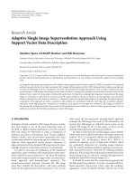
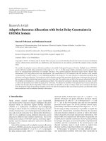
Figure 1: Our smart camera system.
2. SMART CAMERA PARTICLE FILTER TRACKING
We first describe our camera hardware before we go into
the details of particle filter-based tracking in camer a domain
which was presented at ECV05 [21].
2.1. Smart camera hardware description
Our work is based on mvBlueLYNX 420CX smart cameras
from Matrix Vision [22] as shown in Figure 1.Eachsmart
camera consists of a sensor, an FPGA, a processor, and a
networking interface. More precisely, it contains a single
CCD sensor with VGA resolution (progressive scan, 12 MHz
pixel clock) and an attached Bayer color mosaic. A Xilinx
Spartan-IIE FPGA (XC2S400E) is used for low-level pro-
cessing. A 200 MHz Motorola MPC 8241 PowerPC proces-
sor with MMU & FPU running embedded Linux is used for
the main computations. It further comprises 32 MB SDRAM
(64 Bit, 100 MHz), 32 MB NAND-FLASH (4 MB Linux sys-
tem files, approx. 40 MB compressed user filesystem), and
4 MB NOR-FLASH (bootloader, kernel, safeboot system, sys-
tem configuration parameters). The smart camera commu-
nicates via a 100 Mbps Ethernet connection, which is used
both for field upgradeability and parameterization of the sys-
tem and for transmission of the tracking results during run-
time. For direct connection to industrial controls, 16 I/Os are
available. XGA analog video output in conjunction with two
serial ports are available, where monitor and mouse are con-
nected for debugging and target initialization purposes. The

form factor of the smart camera is (without lens) (w
×h×l):
50
×88×75 mm
3
.Itconsumesabout7Wpower.Thecamera
is not only intended for prototyping under laboratory condi-
tions, it is also designed to meet the demands of harsh real
world industrial environments.
2.2. Particle filter
Particle filters can handle multiple hypotheses and nonlin-
ear systems. Following the notation of Isard and Blake [7],
we define Z
t
as representing all observations {z
1
, , z
t
} up
to time t, while X
t
describes the state vector at time t with
dimension k. Particle filtering is based on the Bayes rule to
obtain the posterior p(X
t
| Z
t
) at each time-step using all
available information:
p


X
t
| Z
t

=
p

z
t
| X
t

p

X
t
| Z
t−1

p

z
t

,(1)
whereasthisequationisevaluatedrecursivelyasdescribed
below. The fundamental idea of particle filtering is to ap-
proximate the probability density function (pdf) over X

t
by
aweightedsamplesetS
t
.Eachsamples consists of the state
vector X and a weight π,with

N
i
=1
π
(i)
= 1. Thus, the ith
sample at time t is denoted by s
(i)
t
= (X
(i)
t
, π
(i)
t
). Together they
form the sample set S
t
={s
(i)
t
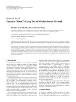
| i = 1, , N}. Figure 2 shows
the principal operation of a particle filter with 8 particles,

whereas its steps are outlined below.
(i) Choose samples step
First, a cumulative histogram of all samples’ weights is com-
puted. Then, according to each particle’s weight π
(i)
t
−1
,its
number of successors is determined according to its relative
probability in this cumulative histogram.
(ii) Prediction step
Our state has the form X
(i)
t
= (x, y, v
x
, v
y
)
(i)
t
. In the predic-
tion step, the new state X
t
is computed:
p

X
t
| Z

t−1

=

p

X
t
| X
t−1

p

X
t−1
| Z
t−1

dX
t−1
. (2)
Different motion models are possible to implement p(X
t
|
X
t−1
). We use three simple motion models (whereas the spec-
ification of how many samples belong to each model can be
parameterized): a random position model, a zero velocity
model, and a constant velocity model (X

t
= AX
t−1
+ w
t−1
),
each enriched with a Gaussian diffusion w
t−1
to spread the
samples and to allow for target moves differing from each
motion model. A combined mode is also implemented where
nonrandom samples belong either to a zero motion model or
a constant velocity model. This property is handed down to
each sample’s successor.
(iii) Measurement step
In the measurement step, the new state X
t
is weighted accord-
ing to the new measurement z
t
(i.e., according to the new
sensor image),
p

X
t
| Z
t

= p


z
t
| X
t

p

X
t
| Z
t−1

. (3)
The measurement step (3) complements the prediction step
(2). Together they form the Bayes formulation (1).
2.3. Color histogram-based particle filter
Measurement step in context of color distributions
As already mentioned, we use a particle filter on the color
histograms. This offers rotation invariant performance and
4 EURASIP Journal on Embedded Systems
[Choose]&[prediction]
deterministic prediction
through motion model
[Diffusion]
[Measurement]
p(X
t
X
t 1

)
p(X
t 1
Z
t 1
)
p(z
t
X
t
)
p(X
t
Z
t
) = p(z
t
X
t
)

p(X
t
X
t 1
)p(X
t 1
Z
t 1
)dX

t 1
Figure 2: Particle filter iteration loop. The size of each sample X
(i)
t
corresponds to its weight π
(i)
t
.
robustness against partial occlusions and nonrigidity. In con-
trast to using standard RGB space, we use an HSV color
model: a 2D Hue-Saturation histogram (HS) in conjunction
with a 1D Value histogram (V) is designed as representa-
tion space for (target) appearance. This induces the following
specializations of the abstract measurement step described
above.
From patch to histogram
Each sample s
(i)
t
induces an image patch P
(i)
t
around its spatial
position in image space, whereas the patch size (H
x
, H
y
)is
user-definable. To further increase the robustness of the color
distribution in case of occlusion or in case of present back-

ground pixels in the patch, an importance weighting depen-
dent on the spatial distance from the patch’s center is used.
We employ the following weighting function:
k(r)
=
⎧
⎨
⎩
1 − r
2
, r<1,
0, otherwise,
(4)
with r denoting the distance from the center. Utilizing this
kernel leads to the color distribution for the image location
of sample s
(i)
t
:
p
(i)
t
[b] = f

wP
(i)
t
k




w −

X
(i)
t


a

δ

I(w) −b

,(5)
with bin number b, pixel position w on the patch, band-
width a
=

H
2
x
+ H
2
y
, and normalization f ,whereas

X
(i)
t

de-
notes the subset of X
(i)
t
which describes the (x, y) position
in the image. The δ-func tion assures that each summand is
assigned to the corresponding bin, determined by its image
intensity I,whereasI stands for HS or V,respectively.The
target representation is computed similarly, so a comparison
to each sample can now be carried out in histogr am space.
From histogram to new weight π
Now we compare the target histogram with each sample’s
histogram. For this, we use the popular Bhattacharyya sim-
ilarity measure [9], both on the 2D HS and the 1D V his-
tograms, respectively:
ρ

p
(i)
t
, q
t

=
B

b=1

p
(i)

t
[b]q
t
[b], (6)
with p
(i)
t
and q
t
denoting the ith sample and target his-
tograms at time t (resp., in Hue-Saturation (HS)andValue
(V) space). Thus, the more similar a sample to the target ap-
pears, the larger ρ becomes. These two similarities ρ
HS
and
ρ
V
are then weighted using alpha blending to get a uni-
fied similarity. The number of bins is variable, as well as
the weighting factor. The experiments are performed using
10
×10 + 10 = 110 bins (H × S + V) and a 70 : 30 weighting
between HS and V . Then, the Bhattacharyya distance
d
(i)
t
=

1 − ρ


p
(i)
t
, q

(7)
is computed. Finally, a Gaussian with user-definable variance
σ is applied to receive the new observation probability for
sample s
(i)
t
:
π
(i)
t
=
1
√
2πσ
exp

−
d
(i)2
t
2σ
2

. (8)
Hence, a high Bhattacharyya similarity ρ leads to a high prob-

ability weight π and thus the sample will be favored more
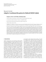
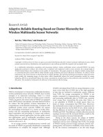
in the next iteration. Figure 3 illustrates how the variance
Sven Fleck et al. 5
0 0.2 0.4 0.6 0.8 1
Bhattacharyya similarity
0
0.5
1
1.5
2
2.5
3
σ
2
(a)
0
0.2
0.4
0.6
0.8
1
Bhattacharyya similarity
0
1
2
3
0
0.2
0.4
0.6

0.8
1
1.2
1.4
Weig ht π
σ
2
(b)
Figure 3: Mapping of Bhattacharyya similarity ρ to weight π for
different variances σ
2
.
σ
2
affects the mapping between ρ and the resulting weight
π. A smaller variance leads to a more aggressive behavior in
that samples with higher similarities ρ arepushedmoreex-
tremely.
2.4. Self-adaptivity
To increase the tracking robustness, the camera automati-
cally adapts to slow appearance (e.g. , illumination) changes
during runtime. This is p erformed by blending the appear-
ance at the most likely position with the actual target refer-
ence appearance in histogram space:
q
t
[b] = α × p
( j)
t
[b]+(1− α) × q

t−1
[b](9)
for all bins b
∈{1, , B} (both in HS and V) using the mix-
ture factor α
∈ [0, 1] and the maximum likelihood sample j,
that is, π
( j)
t
−1
= max
{i=1, ,N}
{π
(i)
t
−1
}. The rate of adaption α is
variable and is controlled by a diag nosis unit that measures
the actual tracking confidence. The idea is to adapt wisely,
that is, the more confident the smart camera about actually
tracking the target itself is, the less the risk of overlearning is
and the more it to the actual appearance of the target adapts.
The degree of unimodality of the resulting pdf p(X
t
| Z
t
)is
one possible interpretation of confidence. For example, if the
target object is not present, this will result in a very uniform
pdf. In this case the confidence is very low and the target rep-

resentation is not altered at all to circumvent overlearning. As
a simple yet efficient implementation of the confidence mea-
sure, the absolute value of the pdf’s peak is utilized, which is
approximated by the sample with the largest weight π
( j)
.
2.5. Smart camera tracking architecture
Figure 4 illustrates the smart camera architecture and its out-
put. In Figure 5 the tracking architecture of the smart camera
is depicted in more details.
2.5.1. Smart camera output
The smart camera’s output per iteration consists of:
(i) the pdf p(X
t
| Z
t
), approximated by the sample set
S
t
={(X
(i)
t
, π
(i)
t
), i = 1, , N}; this leads to (N ∗(k +
1)) values,
(ii) the mean state E[S
t
] =


N
i=1
π
(i)
t
X
(i)
t
,thusonevalue,
(iii) the maximum likelihood state X
( j)
t
with j | π
( j)
t
=
max
N
i
=1
{π
(i)
t
} in conjunction with the confidence π
( j)
t
,
resulting in two values,
(iv) optionally, a region of interest (ROI) around the sam-

ple with maximum likelihood can be transmitted too.
The w hole output is transmitted via Ethernet using sockets.
As only an approximation of the pdf p(X
t
| Z
t
)istransmitted
along with the mean and maximum likelihood state of the
target, our tracking camera needs only about 15 kB/s band-
width when using 100 samples, which is less than 0.33% of
the bandwidth that the transmission of raw images for exter-
nal computation would use. On the PC side, the data can be
visualizedontheflyorsavedonharddiskforoffline evalua-
tion.
2.6. Particle filter tracking results
Before we illustrate some results, several benefits of this smart
camera approach are described.
2.6.1. Benefits
(i) Low-bandwidth requirements
The raw images are processed directly on the camera. Hence,
only the approximated pdf of the target’s state has to be trans-
mitted from the camera using relatively few parameters. This
allows using standard networks (e.g., Ethernet) with virtu-
ally unlimited range. In our work, all the output amounts
to (N
∗ (k + 1) + 3) values per frame. For example, us-
ing N
= 100 and constant velocity motion model (k = 4)
leads to 503 values per frame. This is quite few data com-
pared to transmitting all pixels of the raw image. For exam-

ple (even undemosaiced) VGA resolution needs about 307 k
pixel values per frame. Even at (moderate) 15 fps this al-
ready leads to 37 Mbps tr ansmission rate, which is about 1/3
of the standard 100 Mbps bandwidth. Of course, modern IP
6 EURASIP Journal on Embedded Systems
Target object [histogram]
CCD
With Bayer mosaic
Flash SDRAM
200 MHz
powerPC
processor
+
Spartan IIE
FPGA
Target pdf approximated by samples
pdf pdf
Additional outputs:
Mean estimated state,
Maximum likelihood state & confidence
Ethernet
+low bandwidth I/O
Position (
x, y)
confidence
π 0
50
100 50
0
50

0
0.2
0.4
0.6
0.8
y
x
60 40 20 0 20 40
100
80
60
40
20
0
y
x
Bin
Figure 4: Smart camera architecture.
Smart camera embodiment
p(X
t
Z
t
) = p(z
t
X
t
)p(X
t
Z

t 1
)
Sensor p(z
t
X
t
)
p(X
t
Z
t 1
)
Measurment
step
Prediction
step
p(X
t
Z
t
)
p(X
t 1
Z
t 1
)
p(X
t
X
t 1

)
Networking-/
I/O-unit
p(X
t
Z
t
)
p(X
t
Z
t 1
) =

p(X
t
X
t 1
)p(X
t 1
Z
t 1
)dX
t 1
Figure 5: Smart camera tracking architecture.
cameras offer, for example, MJPEG or MPEG4/H.264 com-
pression which drastically reduces the bandwidth. However,
if the compression is not almost lossless, introduced artefacts
could disturb the further video processing. The smart cam-
era approach instead performs the processing embedded in

the camera on the raw, unaltered images. Compression also
requires additional computational resources which is not re-
quired with the smart camera approach.
(ii) No additional computing outside the camera
has to be performed
No networking enabled external processing unit (a PC or a
networking capable machine control in factory automation)
has to deal with low-level processing any more which algo-
rithmically belongs to a camera. Instead it can concentrate
on higher-level algorithms using all smart cameras’ outputs
as basis. Such a unit could also be used to passively supervise
all outputs (e.g., in case of a PDA with WiFi in a surveillance
application). Additionally, it becomes possible to connect the
output of such a smart camera directly to a machine control
unit (that does not offer dedicated computing resources for
external devices), for example, to a robot control unit for vi-
sual servoing. For this, the mean or the maximum likelihood
state together with a measure for actual tracking confidence
can be utilized directly for real-time machine control.
(iii) Higher resolution and framerate
As the raw video stream does not need to comply with the
camera’s output bandwidth any more, sensors with higher
Sven Fleck et al. 7
spatial or temporal resolutions can be used. Due to the
very close spatial proximity between sensor and process-
ing means, higher bandwidth can be achieved more easily.
In contrast, all scenarios with a conventional vision system
(camera + PC) have major drawbacks. First, transmitting
the raw video stream in ful l spatial resolution at full frame
rate to the external PC can easily exceed today’s networking

bandwidths. This applies all the more when multiple cameras
come into play. Connections with higher bandwidths (e.g.,
CameraLink) on the other hand are too distance-limited (be-
sides the fact that they are typically host-centralized). Sec-
ond, if only regions-of-interest (ROIs) around samples in-
duced by the particle filter were transmitted, the transmis-
sion between camera and PC would become part of the par-
ticle filter’s feedback loop. Indeterministic networking effects
provoke that the particle filter’s prediction of samples’ states
(i.e., ROIs) is not synchronous with the real world any more
and thus measurements are done at wrong positions.
(iv) Multicamera systems
As a consequence of the above benefits, this approach offers
optimal scaling for multicamera systems to work together in
a decentralized way which enables large-scale camera net-
works.
(v) Small, self-contained unit
The smart camera approach offers a self-contained vision so-
lution with a small form fac tor. This increases the reliabil-
ity and enables the install ation at size-limited places and on
robot hands.
(vi) Adaptive particle filter’s benefits
A Kalman filter implementation on a smart camera would
also offer these benefits. However, there are various draw-
backs as it can only handle unimodal pdfs and linear models.
As the particle filter approximates the—potentially arbitrar-
ily shaped—pdf p(X
t
| Z
t

)somewhatefficientlybysamples,
the bandwidth overhead is still moder a te whereas the track-
ing robustness gain is immense. By adapting to slow appear-
ance changes of the target with respect to the tracker’s confi-
dence, the robustness is further increased.
2.6.2. Experimental results
We will outline some results which are just an assortment of
what is also available for download from the project’s web-
site [23] in higher quality. For our first experiment, we ini-
tialize the camera with a cube object. It is trained by pre-
senting it in front of the camera and saving the according
color distribution as target reference. Our smart camera is
capable of robustly following the target over time at a framer-
ate of over 15 fps. For increased computational efficiency, the
tracking directly runs on the raw and thus still Bayer color-
filtered pixels exist. Instead of first doing expensive Bayer de-
mosaicing and finally only using the histogram which still
20 40 60 80 100 120 140
0
50
100
150
200
250
300
(a)
20 40 60 80 100 120 140
0
50
100

150
200
(b)
Figure 6: Experiment no. 1: pdf p(X
t
| Z
t
) over iteration time t.
(a) x-component, (b) y-component.
contains no spatial information, we interpret each four-pixel
Bayer neighborhood as one pixel representing RGB inten-
sity (whereas the two-green values are averaged), leading
to QVGA resolution as tracking input. In the first experi-
ment, a cube is tr acked which is moved first vertically, then
horizontally, and afterwards in a circular way. The final pdf
p(X
t
| Z
t
)attimet from the smart camera is illustrated
in Figure 6,projectedinx and y directions. Figure 7 illus-
trates several points in time in more detail. Concentrating on
the circular motion part of this cube sequence, a screenshot
of the samples’ actual positions in conjunction with their
weights is given. Note that we do not take advantage of the
fact that the camera is mounted statically; that is, no back-
ground segmentation is performed as a preprocessing step.
In the second experiment, we evaluate the performance
of our smart camera in the context of surveillance. The smart
camera is trained w ith a person’s face as target. It shows that

the face can be tracked successfully in real time too. Figure 8
shows some results during the run.
3. 3D SURVEILLANCE SYSTEM
To enable tracking in world model domain, decoupled from
cameras (instead of in the camera image domain), we now
8 EURASIP Journal on Embedded Systems
(a)
(b)
Figure 7: Circular motion sequence of experiment no. 1. Image (a) and approximated pdf (b). Samples are shown in green; the mean state
is denoted as yellow star.
(a)
(b)
Figure 8: Experiment no. 2: face tracking sequence. Image (a) and approximated pdf (b) at iteration no. 18, 35, 49, 58, 79.
extend the system described above as follows. It is based on
our ECV06 work [24, 25].
3.1. Architecture overview
The top-level architecture of our distributed surveillance and
visualization system is given in Figure 9. It consists of multi-
ple networking-enabled camera nodes, a server node and a
3D visualization node. In the following, all components are
described on top level, before each of them is detailed in the
following sections.
Camera nodes
Besides the preferred realization as smart camera, our system
also allows for using standard cameras in combination with
a PC to form a camera node for easier migration from dep-
recated installations.
Server node
The server node acts as server for all the camera nodes and
concurrently as client for the visualization node. It manages

configuration and initialization of all camer a nodes, collects
the resulting tracking data, and takes care of person han-
dover.
Visualization node
The visualization node acts as server, receiving position, size,
and texture of each object currently tracked by any camera
from the server node. Two kinds of visualization nodes are
implemented. The first is based on the XRT point cloud-
rendering system developed at our institute. Here, each ob-
ject is embedded as a sprite in a rendered 3D point cloud of
the environment. The other option is to use Google Earth
as v isualization node. Both the visualization node and the
server node can run together on a single PC.
3.2. Smart camera node in detail
The smart camera tracking architecture as one key compo-
nent of our system is illustrated in Figure 10 and comprises
the following components: a background modeling and auto
init unit, multiple instances of a particle filter-based tracking
unit, 2D
→ 3D conversion units, and a network unit.
3.2.1. Background modeling and autoinit
In contrast to Section 2, we take advantage of the fact that
each camera is mounted statically. This enables the use of a
background model for segmentation of moving objects. The
background modeling unit has the goal to model the actual
Sven Fleck et al. 9
3D surveillance-architecture
Smart camera node
Smart camera node
Camera + PC node

3D visualization node
Server node
Network
Figure 9: 3D surveillance system architecture.
background in real time, that is, foreground objects can be
extracted very robustly. Additionally, it is important, that the
background model adapts to slow appearance (e.g., illumina-
tion) changes of the scene’s background. Elgammal et al. [26]
give a nice overview of the requirements and possible cues to
use within such a background modeling unit in the context of
surveillance. Due to the embedded nature of our system, the
unit has to be very computationally efficient to meet the real-
time demands. State-of-the-art background modeling algo-
rithms are often based on layer extraction, (see, e.g., Torr et
al. [27]) and mainly target segmentation a ccuracy. Often a
graph cut approach is applied to (layer) segmentation, (see,
e.g., Xiao and Shah [28]) to obtain high-quality results.
However, it became apparent, that these algor ithms are
not efficient enough for our system to run concurrently
together with multiple instances of the particle filter unit.
Hence we designed a robust, yet efficient, background algo-
rithm that meets the demands, yet works with the limited
computational resources available on our embedded target.
It is capable of running at 20 fps at a resolution of 320
∗ 240
pixels on the mvBlueLYNX 420CX that we use. The back-
ground modeling unit works on a per-pixel basis. The basic
idea is that a model for the backg round b
t
and an estimator

for the noise process η
t
at the current time t is extr acted from
asetofn recent images i
t
, i
t−1
, , i
t−n
. If the difference be-
tween the background model and the current image,
|b
t
−i
t
|,
exceeds a value calculated from the noisiness of the pixel,
f
1
(η
t
) = c
1
∗ η
t
+ c
2
,wherec
1
and c

2
are constants, the pixel
is marked as moving. This approach, however, would require
storing n complete images. If n is set too low (n<500), a car
stopping at a traffic light, for example, would become part of
the background model and leave a ghost image of the road
as a detected object after moving on because the background
model would have already considered the car as par t of the
scenery itself, instead of an object. Since the amount of mem-
ory necessary to store n
= 500 images consisting of 320∗240
RGB pixels is 500
∗ 320 ∗ 240 ∗ 3 = 115200000 bytes (over
100 MB), it is somewhat impractical.
Instead we only buffer n
= 20 images but introduce a
confidence counter j
t
that is increased if the difference be-
tween the oldest and newest images
|i
t
−i
t−n
| is smaller than
f
2
(η
t
) = c

1
∗ η
t
+ c
3
,wherec
1
and c
3
are constants, or reset
otherwise. If the counter reaches the threshold τ, the back-
ground model is updated. The noisiness estimation η
t
is also
modeled by a counter that is increased by a certain value (de-
fault: 5) if the difference in RGB color space of the actual im-
age to the oldest image in the buffer exceeds the current nois-
iness estimation. The functions f
1
and f
2
are defined as linear
functions mainly due to computational cost considerations
and to limit the number of constants (c
1
, c
2
, c
3
) which need

to be determined experimentally. Other constants, such as τ
which represents a number of frames and thus directly relates
to time, are simply chosen by defining the longest amount of
time an object is allowed to remain stationary before it be-
comes part of the backg round.
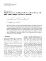
The entire process is illustrated in Figure 11. The current
image i
t
(a) is compared to the oldest image in the buffer i
t−n
(b) and if the resulting difference |i
t
−i
t−n
| (c) is higher than
the threshold f
2
(η
t
) = c
1
∗ η
t
+ c
3
calculated from the noisi-
ness η
t
(d), the confidence counter j
t

(e) is reset to zero, oth-
erwise it is increased. Once the counter reaches a certain level,
it triggers the updating of the background model (f) at this
pixel. Additionally, it is reset back to zero for speed purposes
(to circumvent adaption and thus additional memory oper-
ations at every frame). For illustration purposes, the time it
takes to update the background model is set to 50 frames (in-
stead of 500 or higher in a normal environment) in Figure 11
(see first rising edge in (f)). The background is updated every
time the confidence counter (e) reaches 50. The fluctuations
of (a) up until t
= 540 are not long enough to update the
background model and are hence marked as moving pixels
in (g). This is correct behavior as the fluctuations simulate
objects moving past. At t
= 590 the difference (c) kept low
for 50 frames sustained, so the background model is updated
(in (f)) and the pixel is no longer marked as moving (g). This
simulates an object that needs to be incorporated into the
background (like a parked car). The fluctuations towards the
end are then classified as moving pixels ( e.g., people walking
in front of the car).
Segmentation
Single pixels are first eliminated by a 4-neighborhood ero-
sion. From the resulting mask of movements, areas are con-
structed via a region growing algorithm: the mask is scanned
for the first pixel marked as moving. An area is constructed
around it and its borders checked. If a moving pixel is found
on it, the area expands in that direction. This is done itera-
tively until no border pixel is marked. To avoid breaking up of

10 EURASIP Journal on Embedded Systems
Smart camera architecture
Smart camera node
Sensor Raw image
[Pixel level]
Background
modeling
& autolnit
ROI
ROI
ROI
[Object level]
Particle filter
Particle filter
Particle filter
[Dynamically create/delete
particle filters during runtime
-one filter for each object]
Best
p
X
(i)
t
Best
p
X
(i)
t
Best
p

X
(i)
t
2D 3D
2D 3D
2D 3D
[State level-in camera
coordinates]
p

X
(i)
t
p

X
(i)
t
p

X
(i)
t
Network
unit
Cam
data
[In 3D
world coordinates]
[TCP/IP]

Figure 10: Smart camera node’s architecture.
0 100 200 300 400 500 600 700 800 900 1000
0
400
(1)
(a)
0 100 200 300 400 500 600 700 800 900 1000
0
400
(2)
(b)
0 100 200 300 400 500 600 700 800 900 1000
0
2
10
5
(3)
(c)
0 100 200 300 400 500 600 700 800 900 1000
0
1000
(4)
(d)
0 100 200 300 400 500 600 700 800 900 1000
0
100
(5)
(e)
0 100 200 300 400 500 600 700 800 900 1000
0

400
(6)
(f)
0 100 200 300 400 500 600 700 800 900 1000
0
1
(7)
(g)
Figure 11: High-speed background modeling unit in action. Per
pixel: (a) raw pixel signal from camera sensor. (b) 10 frames old raw
signal. (c) Difference between (a) and (b). (d) Noise process. (e)
Confidence counter: increased if pixel is consistent with background
within a certain tolerance, reset otherwise. (f) Background model.
(g) Trigger event if motion is detected.
objects into smaller areas, areas near each other are merged.
This is done by expanding the borders a certain amount of
pixels beyond the point where no pixels were found moving
any more. Once an area is completed, the pixels it contains
are marked “nonmoving” and the algorithm starts searching
for the next potential area. This unit thus handles the trans-
formation from r aw pixel level to object level.
Auto initialization and destruction
If the region is not already tracked by an existing particle fil-
ter, a new filter is instantiated with the current appearance as
target and assigned to this region. An existing particle filter
that has not found a region of interest near enough over a
certainamountoftimeisdeleted.
This enables the tracking of multiple objects, where each
object is represented by a separate color-based particle filter.
Two particle filters that are assigned the same region of inter-

est (e.g., two people that walk close to each other after meet-
ing) are detected in a last step and one of them is eliminated
if the object does not split up again after a certain amount of
time.
3.2.2. Multiobject tracking—color-based particle filters
Unlike in Section 2, a particle filter engine is instantiated for
each person/object p. Due to the availability of the back-
ground model several changes were made.
(i) The confidence for adaption comes from the back-
ground model as opposed to the pdf’s unimodality.
(ii) The state X
(i)
t
also comprises the object’s size.
(iii) The likeliness between sample and ROI influences the
measurement process and calculation of π
(i)
t
.
3.2.3. 2D
→ 3D conversion unit
3D tracking is implemented by converting the 2D tracking
results in image domain of the camera to a 3D world coor-
dinate system with respect to the (potentially georeferenced)
3D model, which also enables global, intercamera handling
and handover of objects.
Sven Fleck et al. 11
Server node
Server architecture
[Serves as server for camera nodes and as client for visualization server]

[Protocol]
Message
name
Payload
length q
Payload
data
[4 bytes] [4 bytes] [q bytes]
Cam
data
Cam
data
Cam
data
[TCP/IP]
Camera
protocol
[server]
Logfile
Person
handover
unit
XRT
protocol
[client]
XRT
data
[TCP/IP]
[Commands]
[Images]

Camera
GUI
Figure 12: Server architecture.
Since both external and internal camera parameters are
known (manually calibrated by overlaying a virtual rendered
image with a live camera image), we can convert 2D pixel co-
ordinates into world coordinate view rays. The view rays of
the lower left and right corner of the objec t are intersected
with the fixed ground plane. The distance between them de-
termines the width and the mean determines the position
of the object. The height (e.g., of a person) is calculated by
intersecting the view ray from the top center pixel with the
plane perpendicular to the ground plane that goes through
the two intersection p oints from the first step. If the object’s
region of interest is above the horizon, the detected position
lies behind the camera and it will be ignored. The extracted
data is then sent to the server along with the texture of the
object.
3.2.4. Parameter selection
The goal is to achieve the best tracking performance possible
in terms of robustness, precision, and framerate within the
given computational resources of the embedded target. As
the surveillance system is widely parameterizable and many
options affect computational demands, an optimal combina-
tion has to be set up. This optimization problem can be sub-
divided in a background unit and a tracking unit parameter
optimization problem. There are basically three levels of ab-
straction that affec t computational time (bottom up): pixel
level, sample level, and object level operations.
Some parameters, for example, noise, are adapted auto-

matically during runtime. Other parameters that do not af-
fect the computational resources have been set only under
computer vision aspects taking the environment (indoor ver-
sus outdoor) into account. All background unit para meters
and most tracking parameters belong to this class. Most of
these parameters have been selected using visual feedback
from debug images.
Within the tracking unit, especially the number of parti-
cles N is crucial for runtime. As the measurement step is the
most expensive part of the particle filter, its parameters have
to be set with special care. These consist of the number of
histogram bins and the per particle subsampling size which
determines the number of pixels over which a histogram is
built. In practice, we set these par ameters first and finally set
N which linearly affects the tracking units runtime to get the
desired sustained tracking framerate.
3.3. Server node in detail
The server node is illustrated in Figure 12. It consists of a
camera protocol server, a camera GUI, a person handover
unit and a client for the visualization node.
3.3.1. Camera protocol server
The camera server implements a binary protocol for commu-
nication w ith each camera node based on TCP/IP. It serves as
sink for all camera nodes’ tracking result streams which con-
sist of the actual tracking position and appearance (texture)
of every target per camera node in world coordinates. This
information is forwarded both to the person handover unit
and to a log file that allows for debugging and playback of
recorded data. Additionally, raw camera images can be ac-
quired from any camera node for the camera GUI.

3.3.2. Camera GUI
The camera GUI visualizes all the results of any camera node.
The seg mented and t racked objects are overlayed over the
raw sensor image. The update rate can be manually adjusted
to save bandw idth. Additionally, the camera GUI supports
easy calibration relative to the model by blending the ren-
dered image of a virtual camera over the current live image
as basis for optimal calibration, as illustrated in Figure 13.
3.3.3. Person handover unit
To achieve a seamless intercamera tracking decoupled from
each respective sensor node, the person handover unit
merges objects tracked by different camera nodes if they
are in spatial proximity. Obviously, this solution is far from
perfect, but we are currently working to improve the han-
dover process by integrating the object’s appearance, that
12 EURASIP Journal on Embedded Systems
(a) (b) (c)
Figure 13: Camera GUI. Different blending levels are shown: (a) real raw sensor image and (c) rendered scene from same v iewpoint.
L2
L1
C1
(a)
L3
L2
L1
C1
(b)
L3
L2
C1

(c)
Figure 14: Two setups of our mobile platform. (a) Two laser scanners, L1 and L2, and one omnidirectional camera C1. (b), (c) Three laser
scanners, L1, L2, and L3, and omnidirectional camera closely mounted together.
is, comparing color distributions over multiple spatial ar-
eas of the target using the Bhattacharyya distance on color-
calibrated cameras. Additionally, movements over time will
be integrated to further identify correct handovers. At the
moment, the unit works as follows: after a new object has
been detected by a camera node, its tracking position is com-
pared to all other objects that are already being tracked. If an
object at a similar position is found, it is considered the same
object and statically linked to it using its global id.
3.4. Visualization node in detail
A pract ical 3D surveillance system also comprises an easy
way of acquiring 3D models of the respective environment.
Hence, we briefly present our 3D model acquisition system
that provides the content for the visualization node which is
described afterwards.
3.4.1. 3D model acquisition for 3D visualization
The basis for 3D model acquisition is our mobile platform
which we call the W
¨
agele
1
[29]. It allows for an easy ac-
quisition of indoor and outdoor scenes. 3D models are ac-
1
W
¨
agele—Swabian for a little cart.

quired just by moving the platform through the scene to be
captured. Thereby, geometry is acquired continuously and
color images are taken in regular intervals. Our platform (see
Figure 14) comprises an 8 megapixel omnidirectional cam-
era (C1 in Figure 14) in conjunction with three laser scanners
(L1–L3 in Figure 14) and an attitude heading sensor (A1 in
Figure 14). Two flows are implemented to yield 3D models:
a computer vision flow based on graph cut stereo and a laser
scanner based-modeling flow.
After a recording session, the collected data is assembled
to create a consistent 3D model in an automated offline pro-
cessing step. First a 2D map of the scene is built and all scans
of the localization scanner (and the attitude heading sensor)
are matched to this map. This is accomplished by proba-
bilistic scan matching using a generative model developed by
Biber and Straßer [30]. After this step the position and ori-
entation of the W
¨
agele is known for each time step. This data
is then fed into the graph cut stereo pipeline and the laser
scanner pipeline. The stereo pipeline computes dense depth
maps using pairs of panoramic images taken from different
positions. The laser flow projects the data from laser scan-
ners L2 and L3 into space using the results of the localization
step. L2 and L3 together provide a full 360
◦
vertical slice of
the environment. The camera C1, then, yields the texture for
the 3D models. More details can be found in [29, 31].
Sven Fleck et al. 13

(a) (b)
(c) (d) (e)
(f) (g) (h)
(i) (j) (k)
Figure 15: Outdoor setup. (a), (h) Renderings of the acquired model in XRT visualization system. (b) Dewarped example of an omni-
directional image of the model acquisition platform. (c), (f) Live view of camera nodes with overlayed targets currently tracking. (d), (e)
Rendering of resulting person of (c) in XRT visualization system from two viewpoints. (i)–(k) More live renderings in XRT.
3.4.2. 3D visualization framework—XRT
The visualization node gets its data from the server node and
renders the information (all objects currently tracked) em-
bedded in the 3D model. The first option is based on the
experimental rendering toolkit (XRT) developed by Michael
Wand et al. at our institute which is a modular framework
for real-time point-based rendering. The viewpoint can be
chosen arbitrarily. Also a fly-by mode is available that moves
the viewpoint with a tracked person/object. Objects are dis-
played as sprites using live textures. Resulting renderings are
shown in Section 3.5.
3.4.3. Google Earth as visualization node
As noted earlier, our system also allows Google Earth [3]to
be used as visualization node. As shown in the results, each
object is represented with a live texture embedded in the
Google Earth model. Of course, the viewpoint within Google
Earth can be chosen arbitrarily during runtime, independent
of the objects being tracked (and independent of the camera
nodes).
3.5. 3D surveillance results and applications
Two setups have been evaluated over several days, an outdoor
setup and an indoor setup in an office environment. More
details and videos can be found on the project’s website [23].

First, a 3D model of each environment has been acquired.
Afterwards, the camer a network has been set up and cali-
brated relative to the model. Figures 15 and 16 show some
results of the outdoor setup. Even under strong gusts where
the t rees were heavily moving, our p er pixel noise process es-
timator enabled robust tracking by spatially adapting to the
14 EURASIP Journal on Embedded Systems
(a) (b) (c) (d)
Figure 16: Outdoor experiment. (a) Background model. (b) Estimated noise. (c) Live smart camera view with overlayed tracking informa-
tion. (d) Live XRT rendering of tracked object embedded in 3D model.
(a) (b) (c)
(d) (e) (f)
Figure 17: Indoor setup. Renderings of the XRT visualization node. (a), (d) Output of the server node (camera GUI): raw image of the
camera node, overlayed with the target object on which a particle filter is running. (a), (d) Live camera views overlayed by tracking results.
(b), (e) Rendering of embedded live texture in XRT visualization system. (c), (f) Same as center, but with alpha map enabled: only segmented
areas are overlayed for increased realism.
respective backg round movements. Some indoor results are
illustrated in Figure 17. To circumvent strong reflections on
the floor in the indoor setup, halogen lamps are used with
similar directions as the camera viewpoints.
Results of the Google Earth visualization are shown in the
context of the self-localization application on our campus.
Before, experimental results are described.
3.5.1. Long term experiment
We have set up the surveillance system with 5 camera nodes
for long-term indoor operation. It runs 24/7 for 4 weeks now
and shows quite promising performance. Both the 3D visual-
ization within XRT and the Google Earth visualization were
used. Figure 19 illustrates the number of persons tracked
concurrently within the camera network. In Figure 20 the

distribution of number of events per hour within a day is
shown, accumulated over an entire week. The small peak in
the early morning hours is due to a night-watchman. The
peak between 11 AM and 12 PM clearly shows the regular
lunchtime movements on the hallway. Many students leave in
the early afternoon, however as usual in the academic world,
days tend to grow longer and longer, as seen in the figure. As
we do not have an automated way of detecting false tracking
results, no qualitative results showing false object detection
rate are available yet.
3.5.2. Application—self-localization
An interesting application on top of the described 3D surveil-
lance system is the ability to perform multiperson self-
localization w ithin such a distributed network of cameras.
Especially in indoor environments, where no localization
mechanisms like GPS are available; our approach delivers
highly accurate results without the need for special localiza-
tion devices for the user. The scenario looks like this: a user
with a portable computer walks into an unknown building
or airport, connects to the local WiFi network, and down-
loads the XRT v iewer or uses Google Earth. The data is then
streamed to him and he can access the real-time 3D surveil-
lance data feed, where he is embedded as an object. Choosing
the follow option in XRT, the viewer automatically follows
the user through the virtual scene. The user can then navi-
gate virtually through the environment starting from his ac-
tual position.
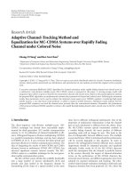
Figure 18 illustr ates a self-localization setup on our cam-
pus. The person to be localized (d) is tracked and visualized
Sven Fleck et al. 15

(a) (b)
(c)
(d)
(e)
(f)
Figure 18: (a) Live view of one camera node where the detected and currently tracked objects are overlayed. (b) Estimated noise of this
camera. Note the extremely high values where trees are moving due to heavy gusts. (c) Overview of the campus in Google Earth, as the
person to be localized sees it. (d) Image of the person being localized with the WiFi-enabled laptop where the visualization node runs. (e)
Same as (c), (f), with XRT used as visualization instrument in conjunction with a georeferenced 3D model acquired by our W
¨
agele platform,
embedded in a low-resolution altitude model of the scene. Note that the 5 objects currently tracked are embedded as live billboard textures.
(f) Close up Google Earth view of (c). Four people and a truck are tracked concurrently. The person to be localized is the one in the bottom
center carrying the notebook.
1234 5678
0
0.1
0.2
0.3
0.4
0.5
0.6
0.7
0.8
Figure 19: Distribution of number of persons concurrently tracked
by the camera network over one week of operation.
in Google Earth (c), (f) and simultaneously in our XRT
point-based renderer (e).
4. CONCLUSION AND FUTURE IDEAS
Our approach of such a distributed network of smart cam-

eras offers various benefits. In contrast to a host central-
ized approach, the possible number of cameras can easily
exceed hundreds. Neither the computation power of a host
nor the physical cable l ength (e.g., like with CameraLink)
is a limiting factor. As the whole tracking is embedded in-
side each smart camera node, only very limited bandwidth
is necessary, which makes the use of Ethernet possible. Ad-
ditionally, the possibility to combine standard cameras and
PCs to form local camera nodes extends the use of PC-based
surveillance over larger areas where no smart cameras are
available yet. Our system is capable of tracking multiple per-
sons in real time. The inter-camera tracking results are em-
bedded as live textures in a consistent and georeferenced 3D
world model, for example, acquired by our mobile platform
or within Google Earth. This enables the intuitive 3D visual-
ization of tracking results decoupled from sensor views and
tracked persons.
One key decision in our system design was to use a dis-
tributed network of smart cameras as this provides vari-
ous benefits compared to a more traditional, centralized ap-
proach as described in Section 2.6.1. Due to real-time re-
quirements and affordability of large installations, we de-
cided to design our algorithms not only on quality but also
on computational efficiency and parameterizability. Hence,
we chose to implement a rather simplistic background mod-
eling unit and a fast particle filtering measurement step.
The detection of a person’s feet turned out to not al-
ways be reliable (which affects the estimated distance from
the camera), also reflections on the floor affected correct lo-
calization of objects. This effect could be attenuated by using

polarization filters. Also, the system fails, if multiple objects
are constantly overlapping each other (e.g., crowds).
16 EURASIP Journal on Embedded Systems
12
am
2
am
4
am
6
am
8
am
10
am
12
pm
2
pm
4
pm
6
pm
8
pm
10
pm
12
am
0

100
200
300
400
500
600
700
800
900
1000
Figure 20: Events over one week, sorted by hour.
Future research includes person identification using
RFID tags, long-term experiments, and the acquisition of en-
hanced 3D models. Additionally, integrating the acquired 3D
W
¨
agele models within Google Ear th will also allow for seam-
less tracking in large, textured 3D indoor and outdoor en-
vironments. However, the acquired models are stil l far too
complex.
Self-localization future ideas
A buddy list could be maintained that goes beyond of what
typical chat programs offer today: the worldwide, georefer-
enced localization visualization of all your buddies instead of
just a binary online/away classification. Additionally, an idea
is that available navig a tion software could be used on top of
this to allow for indoor navigation, for example, to route to
a certain office or gate. In combination with the buddy list
idea, this enables novel services like flexible meetings at un-
known places, for example, within the airport a user can be

navigated to his buddy whereas the buddy’s location is up-
dated during runtime. Also, security personnel can use the
same service to catch a suspicious person moving inside the
airport.
ACKNOWLEDGMENTS
We would like to thank Matrix Vision for their generous sup-
port and successful cooperation, Peter Biber for providing
W
¨
agele data and many fruitful discussions, Sven Lanwer for
his work within smart camera-based tracking, and Michael
Wand for providing the XRT rendering framework.
REFERENCES
[1] J. Mullins, “Rings of steel ii, New York city gets set to replicate
London’s high-security zone,” to appear in IEEE Spectrum.
[2] “What happens in vegas stays on tape,” online.
com/read/090105/hiddencamera
vegas 3834.html.
[3] “Google earth,” />[4] M. Bramberger, A. Doblander, A. Maier, B. Rinner, and
H. Schwabach, “Distributed embedded smart cameras for
surveillance applications,” Computer, vol. 39, no. 2, pp. 68–75,
2006.
[5] W.Wolf,B.Ozer,andT.Lv,“Smartcamerasasembeddedsys-
tems,” Computer, vol. 35, no. 9, pp. 48–53, 2002.
[6]A.Doucet,N.D.Freitas,andN.Gordon,Sequential Monte
Carlo Methods in Practice, Springer, New York, NY, USA, 2001.
[7] M. Isard and A. Blake, “Condensation—conditional density
propagation for visual tracking,” International Journal of Com-
puter Vision, vol. 29, no. 1, pp. 5–28, 1998.
[8] S. Haykin and N. de Freitas, “Special issue on sequential state

estimation,” Proceedings of the IEEE, vol. 92, no. 3, pp. 399–
400, 2004.
[9] D. Comaniciu, V. Ramesh, and P. Meer, “Kernel-based object
tracking,” IEEE Transactions on Pattern Analysis and Machine
Intelligence, vol. 25, no. 5, pp. 564–577, 2003.
[10] K. Okuma, A. Taleghani, N. de Freitas, J. J. Little, and D.
G. Lowe, “A boosted particle filter: multitarget detection and
tracking,” in Proceedings of 8th European Conference on Com-
puter Vision (ECCV ’04), Prague, Czech Republic, May 2004.
[11] K. Nummiaro, E. Koller-Meier, and L. V. Gool, “A color based
particle filter,” in Proceedings of the 1st International Workshop
on Generative-Model-Based Vision (GMBV ’02), Copenhagen,
Denmark, June 2002.
[12] P. P
´
erez, C. Hue, J. Vermaak, and M. Gangnet, “Color-based
probabilistic tracking,” in Proceedings of 7th European Confer-
ence on Computer Vision (ECCV ’02), pp. 661–675, Copenh-
aguen, Denmark, June 2002.
[13] P. P
´
erez, J. Vermaak, and A. Blake, “Data fusion for visual
tracking with particles,” Proceedings of the IEEE, vol. 92, no. 3,
pp. 495–513, 2004, issue on State Estimation.
[14] M. Spengler and B. Schiele, “Towards robust multi-cue inte-
gration for visual tracking,” in Proceedings of the 2nd Interna-
tional Workshop on Computer Vision Systems , vol. 2095 of Lec-
ture Notes in Computer Science, pp. 93–106, Vancouver, BC,
Canada, July 2001.
[15] “Surveillance works: look who’s watching,” IEEE Signal Pro-

cessing Magazine, vol. 22, no. 3, 2005.
[16] T. Boult, A. Lakshmikumar, and X. Gao, “Surveillance
methods,” in Proceedings of IEEE Computer Society Interna-
tional Conference on Computer Vision and Pattern Recognition
(CVPR ’05), San Diego, Calif, USA, June 2005.
[17] N. Siebel and S. Maybank, “The advisor visual surveillance sys-
tem,” in Proceedings of the ECCV Workshop on Applications of
Computer Vision (ACV ’04), Prague, Italy, May 2004.
[18] M. M. Trivedi, T. L. Gandhi, and K. S. Huang, “Distributed
interactive video arrays for event capture and enhanced situ-
ational awareness,” IEEE Intelligent Systems,vol.20,no.5,pp.
58–65, 2005, special issue on Homeland Security, 2005.
[19] D.B.Yang,H.H.Gonz
´
alez-Ba
˜
nos, and L. J. Guibas, “Count-
ing people in crowds with a real-time network of simple image
sensors,” in Proceedings of the 9th IEEE International Confer-
ence on Computer Vision (ICCV ’03), vol. 1, pp. 122–129, Nice,
France, October 2003.
[20] H. S. Sawhney, A. Arpa, R. Kumar, et al., “Video flashlights—
real time rendering of multiple videos for immersive model vi-
sualization,” in Proceedings of the 13th Eurographics Workshop
on Rendering (EGRW ’02), pp. 157–168, Pisa, Italy, June 2002.
[21] S. Fleck and W. Straßer, “Adaptive probabilistic tracking em-
bedded in a smart camera,” in Proceedings of the IEEE CVPR
Embedded Computer Vision Workshop (ECV ’05), vol. 3, p. 134,
San Diego, Calif, USA, June 2005.
[22] “Matrix vision,” />[23] “Project’s website,” />∼sfleck/

smartsurv3d/.
Sven Fleck et al. 17
[24] S. Fleck, F. Busch, P. Biber, and W. Straßer, “3d surveillance—
a distributed network of smart cameras for real-time tracking
and its visualization in 3d,” in Proceedings of IEEE CVPR Em-
bedded Computer Vision Workshop (ECV ’06), 2006.
[25] S. Fleck, F. Busch, P. Biber, and W. Straßer, “3d surveillance—
a distributed network of smart cameras for real-time track-
ing and its visualization in 3d,” in Proceedings of Confer-
ence on Computer Vision and Pattern Recognition Workshop
(CVPRW ’06), p. 118, June 2006.
[26] A. Elgammal, R. Duraiswami, D. Harwood, and L. S. Davis,
“Background and foreground modeling using nonparametric
kernel density estimation for visual surveillance,” Proceedings
of the IEEE, vol. 90, no. 7, pp. 1151–1162, 2002.
[27] P. H. S. Torr, R. Szeliski, and P. Anandan, “An integ rated
Bayesian approach to layer extraction from image sequences,”
IEEE Transactions on Pattern Analysis and Machine Intelligence,
vol. 23, no. 3, pp. 297–303, 2001.
[28] J. Xiao and M. Shah, “Motion layer extraction in the presence
of occlusion using graph cuts,” IEEE Transactions on Pattern
Analysis and Machine Intelligence, vol. 27, no. 10, pp. 1644–
1659, 2005.
[29] P. Biber, S. Fleck, M. Wand, D. Staneker, and W. Straßer, “First
experiences with a mobile platform for flexible 3d model ac-
quisition in indoor and outdoor environments—the w
¨
agele,”
in Proceedings of the ISPRS Working Group V/4 Workshop 3D-
ARCH 2005: Virtual Reconstruction and Visualization of Com-

plex Architectures (ISPRS ’05), Mestre-Venice, Italy, August
2005.
[30] P. Biber and W. Straßer, “The normal distributions transform:
a n ew approach to laser scan matching,” in Proceedings of the
IEEE/RSJ International Conference on Intelligent Robots and
Systems (IROS ’03), vol. 3, pp. 2743–2748, Las Vegas, Nev,
USA, October 2003.
[31]S.Fleck,F.Busch,P.Biber,H.Andreasson,andW.Straßer,
“Omnidirectional 3d modeling on a mobile robot using
graph cuts,” in Proceedings of the IEEE International Confer-
ence on Robotics and Automation (ICRA ’05), pp. 1748–1754,
Barcelona, Spain, April 2005.