Báo cáo hóa học: " Stochastic Oscillations in Genetic Regulatory Networks: Application to Microarray Experiments" docx

Hindawi Publishing Corporation
EURASIP Journal on Bioinformatics and Systems Biology
Volume 2006, Article ID 59526, Pages 1–12
DOI 10.1155/BSB/2006/59526
Stochastic Oscillations in Genetic Regulatory Networks:
Application to Microarray Experiments
Simon Rosenfeld
Division of Cancer Prevention, Biometry Research Group, National Cancer Institute, Bethesda, MD 20892, USA
Received 19 January 2006; Revised 26 June 2006; Accepted 27 June 2006
Recommended for Publication by Yue Wang
We analyze the stochastic dynamics of genetic regulatory networks using a system of nonlinear differential equations. The system
of S-functions is applied to capture the role of RNA polymerase in the transcription-translation mechanism. Using probabilistic
properties of chemical rate equations, we derive a system of stochastic differential equations which are analytically tractable despite
the high dimension of the regulatory network. Using stationary solutions of these equations, we explain the apparently paradoxical
results of some recent time-course microarray experiments where mRNA transcription levels are found to only weakly correlate
with the corresponding transcription rates. Combining analytical and simulation approaches, we determine the set of relation-
ships between the size of the regulatory network, its structural complexity, chemical variability, and spectrum of oscillations. In
particular, we show that temporal variability of chemical constituents may decrease while complexity of the network is increasing.
This finding provides an insight into the nature of “functional determinism” of such an inherently stochastic system as genetic
regulatory network.
Copyright © 2006 Simon Rosenfeld. This is an open access article distributed under the Creative Commons Attribution License,
which permits unrestricted use, distribution, and reproduction in any medium, provided the original work is properly cited.
1. INTRODUCTION
According to the “central dogma” in molecular biology, the
genetic regulatory process involves two key steps, namely,
“transcription,” that is, deciphering the genetic code and cre-
ation of the messenger RNA (mRNA), and “translation,” that
is, synthesis of the proteins by ribosomes using the mRNAs
as templates. These processes run concurrently for all the
genes comprising the genome. Importantly, each molecular
assembly responsible for deciphering the genetic code is itself

built from the proteins produced through transcription and
translation of other genes, thus introducing nonlinear inter-
actions into the regulator y process (Lewin [1]). In the human
genome, for example, from 30 to 100 regulatory proteins are
usually involved in each transcription event in each of about
30,000 genes. This means that the regulatory network is si-
multaneously of a very high dimensionality and very high
connectivity. Mathematical description of such a network
is a challenging task, both conceptually and computation-
ally. Quite paradoxically, however, this seemingly unfavor-
able combination of two “highs” opens a new avenue for ap-
proximate solutions and understanding the g lobal behavior
of regulatory systems through the application of asymptotic
methods. The novelty introduced by our model is that it does
not simplify the processes through decreasing the dimen-
sionality. On the contrar y, the model takes advantage of the
system being asymptotically large.
In this paper, we pay special attention to quantitative re-
lations between the transcription levels (TLs), that is, the
numbersofmRNAmoleculesofacertaintypepercell,and
transcription rates (TRs), that is, the numbers of mRNA
molecules produced in the cell per unit of time. TLs are
the quantities directly derived from microarray experiments,
whereas TRs are usually unobservable. Although both of
these quantities seem to be legitimate indicators for charac-
terizing gene activity, generally they are different and cap-
ture different facets of the regulatory mechanism. The fun-
damentally nonlinear nature of the gene-to-gene interactions
precludes any direct relations between gene-specific TRs and
TLs. Also, due to the inherent instability of high-dimensional

regulatory systems, nothing like time-independent “gene ac-
tivity” may be att ributed to a living cell. In our view, these
conclusions may have serious consequences for the inter-
pretation of microarray experiments where the fluctuating
2 EURASIP Journal on Bioinformatics and Systems Biology
nature of the mRNA levels is frequently ignored, mRNA
abundance is often seen as a direct indicator of the corre-
sponding gene’s activity, and the differential expression (i.e.,
difference in TLs) is taken as evidence of differences in the
cells themselves.
2. ASSUMPTIONS AND EQUATIONS
The system of nonlinear ordinary differential equations for
the description of proteome-transcriptome dynamics first
appeared in [2]
dr
dt
= F(p) − βr,
dp
dt
=γr−δp,(1)
where r and p are n-dimensional column vectors of mRNA
and protein concentrations measured in numbers of copies
per cell; n is the number of genes in genome; β, γ,andδ are
nondegenerate diagonal matrices corresponding to the rates
of production and degradation in transcription and transla-
tion. The n-dimensional vector-function, F(p), is a strongly
nonlinear function representing the mechanism of transcrip-
tion. Chen et al. [2] l inearized the system (1) in the vicinity
of a certain hypothesized initial point and formulated gen-
eral requirements of stability. In what follows, we augment

the system (1) by an explicitly specified model for F(p)and
attempt to extract the consequences from the essentially non-
linear nature of the problem. Note that according to com-
monly accepted terminology of chemical kinetics (Zumdahl
[3]), production rate is defined as the number of molecules
produced in the system per unit of time. It may or may not
be balanced by an opposite process of degradation. Because
transcription is the process of production of mRNA, we refer
to the quantity F(p)astranscription rate.
As is known from the biology of gene expression, gen-
erationofeachcopyofmessengerRNAisprecededbya
complex sequence of events in which a large number of pro-
teins bind to the gene’s regulatory sites and assemble a read-
ing mechanism known as RNA polymerase (RNAP) (Kim
et al. [4]). Each binding represents a separate biochemi-
cal reaction involving DNA and proteins and is supported
by a number of enzymes and smaller molecules. Accord-
ing to the principles of chemical kinetics, the production
term, F(p), should have the following general form (De Jong
[5])
F
i

p
1
, , p
n

=
L

i

k=1
ω
ik
n

m=1
p
r
ikm
m
,(2)
where L
i
is the number of concurrent biochemical reactions
for decoding the ith gene; ω
ik
are the rate constants; and r
ikm
are the kinetic orders showing how many protein molecules
of type m participate in kth biochemical reaction for the
transcription of ith gene. A detailed account of the assump-
tions underlying (2)maybefoundin[6]. Although these as-
sumptions are not free from inevitable simplifications, they
constitute a reasonably solid basis for studying the dynam-
ics of genetic regulatory networks because they recognize
the central role of RNAPs in the nonlinear mechanism of
gene-to-gene interactions. However, it should be unequivo-
cally stated that many secondary mechanisms of regulation

remain beyond the scope of this model. For example, sys-
tem (1) depicts an important process of mRNA degradation
as the first-order chemical reaction. This suggests the idea
that the proteins controlling the ribosomes do not return
back to the genetic regulatory network and do not become
the parts of the deciphering assemblies again. Of course, this
is a comparatively crude representation of a more complex
process which takes place in reality (Maquat [7]). However,
inclusion of this and similar processes into the model does
not amount to a new mathematical problem because the sys-
tem (1)-(2) may be easily augmented by additional terms
expressed through the S-function in the same manner as
in (2).
Although the biochemical nature of gene expression can-
not be doubted, applicability of the standard concepts and
descriptors of chemical kinetics to these processes is not
out of question. For example, the process that is commonly
compartmentalized as “binding” of a protein to the regula-
tory site is, in fact, a sequence of events of enormous com-
plexity involving a large number of transcriptional coacti-
vators. In a sense, each such binding is a unique adven-
ture which cannot be directly characterized in terms of con-
stant gene-specific chemical rates and stoichiometric coeffi-
cients (Lemon and Tjian [8]). The processes of synthesis of
the RNAPs may be schematically subdivided into a sequence
of steps and rearrangements which may be thought, again
with a certain degree of abstraction, as separate biochemi-
cal reactions. That is why it is admissible to say that there
are many chemical reactions between the proteins and the
DNA molecule which run concurrently within the same reg-

ulatory site. However, one needs to be careful with exces-
sively straightforward application of standard biochemical
terminology and quantitative parameterization to such pro-
cesses, only in principle similar to simple biochemical reac-
tions.
3. STOCHASTICITY IN GENETIC
REGULATORY NETWORKS
There is a large body of theoretical and experimental works
devoted to various aspects of randomness and stochasticity
in coupled biochemical systems. We briefly summarize some
of the key facts here.
As indicated by Gillespie [9], “the temporal behavior of
a chemically reacting system of classical molecules is a deter-
ministic process in the 2N position-momentum phase space,
but it is not a deterministic process in the N-dimensional
subspace of the species population numbers. Therefore, both
reactive and non-reactive molecular collisions are intrinsi-
cally random processes characterized by the collision proba-
bility per unit of time. That is why these collisions constitute
a stochastic Markov process, rather than a deterministic rate
process.”
Simon Rosenfeld 3
Elf and Ehrenberg [10] observe that “the copy num-
bers of the individual messenger RNAs can often be ver y
small, and this frequently leads to highly significant rela-
tive fluctuations in messenger RNA copy numbers and also
to large fluctuations in protein concentrations.” In addi-
tion, there are inevitable statistical variations in the random
partitioning of small numbers of regulatory molecules be-
tween daughter cells when cells divide (McAdams and Arkin

[11]).
McAdams and Arkin [12] indicate that “time delays re-
quired for protein concentration growth depend on environ-
mental factors and availability of a number of other pro-
teins, enzymes and supporting molecules. As a result, the
switching delays for genetically coupled links may widely
vary across isogenic cells in the population. One consequence
of these differingtimesbetweencelldivisionsisprogres-
sive desynchronization of initially synchronized cell popula-
tions. Within a single cell, random variations in duration of
events in each cell-cycle controlling path will lead to unco-
ordinated variations in relative timing of equivalent cellular
events.”
Multiple closely spaced ribosomes may process the same
strand of mRNA simultaneously. Because the spacing s be-
tween ribosomes are random, the number of proteins trans-
lated from the same transcript may also fluctuate randomly
(McAdams and Arkin [11]).
Recent experiments (Cai et al. [13]) demonstrated that
even in an individual cell, the production of a protein and
supporting enzy mes is a stochastic process following a com-
plex pattern of bursting with random distribution of intensi-
ties and durations. Similarly, Rosenfeld et al. [14] found that
quantitative relations between transcription factor concen-
trations and the rate of protein production fluctuate dramat-
ically in the individual living cells, thereby limiting the ac-
curacy with which genetic transcription circuits can trans-
fer signals. The processes mentioned above represent vari-
ous facets of the natural stochasticity of intracellular regu-
latory systems. In addition, stochastic concepts are engaged

as the way of describing extremely intricate quasi-chaotic
behavior, even if the system is fully deterministic in prin-
ciple. As demonstrated by famous examples of the Lorenz
attractor (Lorenz [15]), Belousov-Zhabotinsky autocatalytic
reactions (Zhang et al. [16]), Lotka-Volterra population dy-
namics (Lotka [17]), and many other examples (Bower and
Bolouri [18]), chaotic behavior may appear even in low-
dimensional systems with rather simple structure of non-
linearity. On the contrary, the intracellular biochemical net-
works are high-dimensional systems with a very complex
structure of nonlinearity. These properties make it difficult to
overcome mathematical problems without substantial sim-
plifications. In statistical mechanics, a traditional way of for-
mulating a complex multidimensional problem is to intro-
duce the concept of statistical ensemble (Gardiner [19]). In
high-dimensional biochemical network there are many ways
to introduce a statistical ensemble, but those are preferable
that provide tangible mathematical advantages combined
with intuitive clarity and ease of interpretation, as discussed
below.
The rate constants, ω
ik
, and kinetic orders, r
ikm
,are
assumed to be time-independent positive real and integer
numbers, respectively. For computational purposes, we spec-
ify them as random numbers drawn from the gamma and
Poisson populations, respectively:
Pr


ω
ik
= x

=
x
α−1
exp(−x/θ)
Γ(α)θ
α
,
Pr

r
ikm
= n

=
λ
n
exp(−λ)
n!
.
(3)
This choice of probabilistic characterization is a matter of
mathematical convenience and may be easily replaced by
other assumptions compatible with the nature of the prob-
lem. Similar to random Boolean networks (Kauffman et
al. [20]), the network introduced in (1)–(3) is a collection of

identical regulatory units with random assignment of func-
tional properties controlled through the parameters ω
ik
and
r
ikm
. To avoid a possible misconception, it should be noted
that the statistical ensemble introduced through (3)isnot
intended to mimic a group of isogenic cells. Even less so,
the ensemble (3) may be interpreted as a group of neigh-
boring cells in the same tissue because there is always a cer-
tain degree of cooperativity and synchronization between the
cells under the control of higher loops of regulation (Ptashne
[21]). Therefore, these cells will not represent statistically in-
dependent members of ensemble. Rather, the ensemble (3)
represents the collection of all possible networks of sim-
ilar types sharing the same probabilistic structure. Simu-
lation experiments show that both summary statistics and
global time-independent parameters of such networks gen-
erated in independent runs are identical for practical pur-
poses for those networks with size above several hundred
regulatory units. Such a notion of statistical ensemble is
analogous to that in statistical physics. The states of dif-
ferent members of the ensemble (say, the volumes of ideal
gas enclosed in the thermostats with the same tempera-
ture) are not supposed to be similar to each other at any
fixed moment in time because the t rajectories in their re-
spective phase spaces may be entirely different. However,
what the members of ensemble do have in common are the
integral time-independent statistical characteristics of these

trajectories.
The usage of parameterization (3) in this work is twofold.
First, it serves as a concise method for generating the net-
work structure in simulation experiments. In the context of
this research, we are not interested in peculiarities of the net-
work behavior associated with any specific selection of the
coefficients. Rather, we are interested in exploration of global
behavior of the whole class of the networks sharing the same
probabilistic structure. The second usage of (3) in this work
is of purely technical nature. It often happens that the results
of mathematical calculations are expressed in terms of sum-
mary statistics of the parameters characterizing the system. If
the system is asymptotically large, then these summary statis-
tics can be directly related to their expected values, thus al-
lowing for representation of the results in a concise, easily
comprehensible form.
4 EURASIP Journal on Bioinformatics and Systems Biology
4. OUTLINE OF THE SOLUTION
We seek a stationary solution of the system (1). To envision
a general structure of this solution, we invoke considerations
of the theory of stability of differential equations (Carr [22]).
Following standard methodology, we first seek the equilib-
rium (fixed) point of (1)-(2) and try to determine whether
the solution in its vicinity is stable or unstable. Let P
0
be
the n-vector of equilibrium protein concentrations, and X(t)
be the vector of relative concentrations normalized by these
equilibrium values. After some transformation, system (1)-
(2)mayberewrittenas

¨
x
i
+

β
i
+ δ
i

˙
x
i
+ β
i
δ
i
x
i
= β
i
δ
i
L
i

k=1
Ω
ik
Y

ik
,(4)
where Y are the S-functions (Savageau and Voit [23]) defined
as
log Y
ik

x
1
, , x
n

=
n

k=1
r
ikm
log x
m
,(5)
Ω
ik
=
ω
ik
Y
ik

P

0


L
i
k=1
ω
ik
Y
ik

P
0

(6)
(note that by definition

L
i
k=1
Ω
ik
= 1). System (4)isstrongly
nonlinear, and there are no reasons to hope that its solution
may be obtained in some closed form. However, some im-
portant elements of the solution may be understood with
the help of the center manifold theory (Perko [24]). A de-
tailed discussion of the application of this theory to biochem-
ically motivated S-systems may be found in Lewis [25]. An
informal statement of this theory is that in close vicinity of

the equilibrium, the trajectories residing in stable and un-
stable manifolds (i.e., those associated with eigenvalues of
the Jacobian matrix residing in the left and right halves of
the complex plane, resp.) are topologically homeomorphic
to the corresponding trajectories of the linear system. The
solutions associated with the purely imaginary eigenvalues
(which would be quasi-periodic in the linear theor y) become
the sources of extremely intricate chaotic behavior, but im-
portantly these solutions are bounded, thus representing a
sort of stationary random-like process. Note that in practical
applications it is not usually required that the real parts of
the roots in the center manifold are to be exactly zero, they
only need to be small enough to justify ignoring nonstation-
arity during the life time of the process under consideration
(Bressan [26]). There are numerous attempts in the litera-
ture to describe the oscillatory behavior of genetic regulatory
networks in a linear fashion using the concept of feedback
loops and other methods widely applied in the control theory
(Chen et al. [2]; Wang et al. [27]). Unfortunately, the issue
of stability of such oscillatory regimes is extremely difficult
to explore within the linear theory; therefore, the require-
ments of stability are to be imposed on the matrix of coeffi-
cients of the linear system. These requirements lead to a set of
very complex relationships between coefficients, and it is far
beyond the capabilities of existing theories to elucidate a nat-
ural mechanism, biochemical, or other, which would surely
maintain these relationships throughout the regulatory pro-
cess. In light of the above described inherent stochastisity
of gene expression, the very existence of such a mechanism
seems unlikely. However, postulating a fundamentally non-

linear nature of the problem is out of the question. This is
seen from the very fact that the “hardware” of the processes
underlying gene expression is predominantly the system of
biochemical reactions, and, as such, they are adequately de-
scribed by the nonlinear equations of chemical kinetics. We
therefore make the point that the oscillatory behavior of ge-
netic regulatory networks is possible not in spite of but rather
owing to the nonlinearity of the system. This means that the
nonlinear effects are able to self-organize themselves in such
a manner as to automatically keep the system somewhere in
close vicinity of the linear oscillatory regime. In what follows,
we show that such a scenario is conceivable.
Qualitatively, the approach to the solution of (4)isbased
on the following two heuristic considerations. First, we draw
attention to the “mixing property” of S-functions which may
be explained as follows. Suppose that each of x
1
(t), , x
n
(t)
is represented by linear superpositions of simple periodic
processes with a certain set of frequencies. The “forcing”
functions in the right-hand side of (4) are the multivari-
ate polynomials of those quasi-periodic processes contain-
ing numerous combinatory frequencies along with the origi-
nal ones; as such these form essentially continuous spectra of
the forcing terms. We can reasonably consider functions with
such a complex behavior as stochastic processes. Obviously,
functions (2) become even more chaotic if the arguments
x

1
(t), , x
n
(t) are themselves the random processes. On the
other hand, in a system having high dimension and a high
degree of nonlinearity, deterministic solutions of (4), even
if available, would be completely useless. That is why at the
very outset we abandon the idea of obtaining the determin-
istic solutions and assume that x
1
(t), , x
n
(t) are stationar y
stochastic processes. To this end, the goal of the solution of
system (4) is reduced to determination of the statistical char-
acteristics of these processes. To obtain these characteristics,
we notice that the right-hand side in (5)isthesumofran-
dom variables satisfying Lindeberg’s conditions (essentially,
boundness of the moments: e.g., Loeve [28]). We also allow
the random processes x
1
(t), , x
n
(t) to be weakly dependent
and satisfy the so-called strong mixing conditions (Bradley
[29]). The latter assumption is difficult to substantiate the-
oretically but easy to demonstrate by simulation under the
assumptions of our model. Based on these assumptions, we
may conclude that the sums in (5) are asymptotically normal,
and therefore the random processes η

ik
(t) = log Y
ik
[X(t)]
are approximately Gaussian. The second heuristic consider-
ation we engage is that the random forces corresponding to
different genes are basically nonlinear combinations of the
same set of variables and therefore, generally speaking, are
correlated with each other. Figure 1 illustrates this premise
(see Appendix A for more details). In this figure, (a) shows
100 separate quasi-periodic oscillations covering a wide
spectrum of frequencies formed from the center manifold
Simon Rosenfeld 5
0 2040 6080100
1
0.5
0
0.5
1
Time
Protein oscillations
(a)
0 2040 6080100
1
0.5
0
0.5
1
Time
Transcription rate

(b)
Figure 1: Nonlinear transformation of linear combination of peri-
odic oscillations.
eigenvalues. As shown in (b), corresponding functions
F
i
(P(t)) in (2) tend to concentrate around a certain stochastic
process which is identical for all the genes. This kind of “co-
herence,” that is, the tendency to tightly concentrate around
a common limiting process increases as the complexity of the
network increases. Statistical analysis shows that the limiting
process may be adequately represented as a Gaussian ran-
dom process. Based on this observation, we assume that all
the processes, η
ik
(t), corresponding to different indexes i and
k may be replaced by a single Ornstein-Uhlenbeck process
(Gardiner [19]), that is, by the process described by the Ito
stochastic differential equation (SDE)
dη
t
=−η
dt
τ
0
+

2
τ
0

σdW
t
,(7)
where W
t
is the unit Wiener process. Considering the asymp-
totic normality and computing the time averages of both
sides in (5), we find that the autocovariance of this process
is
R
η
(τ) =

λ
2
+ λ

n

k=1
σ
2
m
exp

−|
τ|/τ
0

,(8)

where σ
2
m
= var[ln(x
m
)] (see Appendix B for details). The
correlation radius, τ
0
, can be easily estimated computation-
ally through fitting η
t
by the first order (i.e., Markov) process.
System (4) is now decoupled on the set of independent
equations containing the same “random force,” exp[η(t)],
¨
x
i
+

β
i
+ δ
i

˙
x
i
+ β
i
δ

i
x
i
= β
i
δ
i
exp

η(t)

. (9)
Because the process η(t) is presumed to be Gaussian, the pro-
cess ξ(t)
= exp[η(t)] is lognormally distributed with the ex-
pectation exp[σ
2
/2] and v ariance exp(σ
2
)[exp(σ
2
) − 1]. To
determine the temporal structure of its autocovariance, we
first derive SDE for ξ(t)from(7) and, after some unessential
simplifications, find
R
e
(τ) = exp

σ

2

exp

σ
2

− 1

exp

−
τ
τ
0
σ
2
1 − exp

−
σ
2


,
(10)
where
σ
2
=


λ
2
+ λ

n

m=1
var

log

x
m

. (11)
Comparing (10)and(8), we notice that the correlation ra-
dius of the process ξ(t) is always smaller than that of η(t),
which means that ξ(t) is always closer to white noise than
η(t). Applying a Fourier transform, (9) can now be easily
solved, and the solutions are the stochastic processes with ex-
pectations
E

x
i

=
β
i

δ
i
exp

σ
2
/2

, (12)
variances
var

x
i

=
β
i
δ
i
β
i
+ δ
i
τ
0

exp

σ

2

−
1

2
σ
2
, (13)
and autocorrelation function
R
i
(τ) = A
i
exp

−|τ|/τ
0

+ B
i
exp

− β
i
|τ|

+ Δ
i
exp


−
δ
i
|τ|

(14)
(see Appendix C for details).
The variance, σ
2
, should satisfy the conditions of self-
consistency derived from the combination of (11)and(13).
Simple algebra leads to the transcendental algebraic equation
σ
2
=

λ
2
+ λ

n

i=1
ln

1+2τ
0
β
i

δ
i
β
i
+ δ
i
cosh σ
2
− 1
σ
2

. (15)
In a sense, the solution of the original strongly nonlinear
problem is now reduced to solving this equation. Substitu-
tion of σ
2
into (12) concludes the procedure of solving the
system (4).
5. INTERRELATIONS BETWEEN NONLINEARITY,
STABILITY, AND COMPLEXITY
Parameter λ in the Poisson distribution (3)isanaturalmea-
sure of the complexity of the system. This is because the
quantity λn can be interpreted as the average (per gene)
number of the proteins participating in the act of transcrip-
tion. We now formally introduce the “index of complexity,”
I
c
= (λ
2

+ λ)n. If this index were small, then the vast ma-
jority of characteristic roots of the Jacobian matrix would be
stable, that is, have negative real parts (see Appendix D for
some details regarding characteristic roots). Obviously, this
is not the case in reality with I
c
usually somewhere between
30 and 100 (Lewin [1]). In the system of such great com-
plexity, a substantial number of the characteristic roots will
reside in the right half of the complex plane, thus signifying
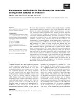
6 EURASIP Journal on Bioinformatics and Systems Biology
6 4 20246
6
4
2
0
2
4
6
Real parts
Imaginary parts
n = 300 ; Poisson λ = 0.05 ; spectral width = 2.21;
complexity index
= 15.75 ; stability index = 3.47
Figure 2: Positions of characteristic roots in case of low complexity.
greater instability of linear oscillatory regime. For this rea-
son, we also define the “index of stability,” I
s
, assuming that
it is the ratio of the number of roots with negative real parts

to those with positive ones. Intuitively, it is quite obvious
that a certain relationship should exist between the stabil-
ity, complexity, and spectral width of center manifold. This
kind of relationship is not easy to derive theoretically but is
fairly easy to demonstrate by simulation (Appendix E). Two
examples of the distribution of the characteristic roots over
the complex plane for small and large I
c
are shown in Fig-
ures 2 and 3, respectively. With complexity increasing, the
stability decreases, the spectral width of the central mani-
fold increases, thus making the correlation radius, τ
0
,smaller
and the spectrum of collective “random force,” ξ(t), “whiter.”
Effectively, this means that the more complex the system is,
the more favorable the conditions are for applying the pro-
posed approach. Figure 4(a) demonstrates that stability de-
creases when complexity increases. Figure 4(b) illustrates the
fact that the correlation radius of ξ(t) (open circles) is always
substantially smaller than that of η(t) (solid circles) and both
drastically decrease with increasing I
c
.
6. INTERRELATIONS BETWEEN TRANSCRIPTION
LEVELS AND TRANSCRIPTION RATES
In the model adopted here, the entire gene expression mech-
anism is seen as being driven by a collective random force
which in turn is generated by all the individual transcription-
translation e vents. This kind of “self-consistent” or “average

field” approach is widely employed in physics, with such no-
table examples as Thomas-Fermi equation in atomic physics
(Parr and Yang [30]) and Landau-Vlasov equations in the
physics of plasma (Chen [31]),tonamejustafew.Tran-
scription levels (TLs) and transcription rates (TRs) are rep-
resented by the quantities r
i
and F
i
in (1), respectively. In
general, since F
i
are the stochastic processes generated by the
entire network, there are no noticeable correlations between
them and any of r
i
. Therefore, one cannot expect any sub-
stantial similarity between the temporal behavior of TRs and
6 4 20246
6
4
2
0
2
4
6
Real parts
Imaginary parts
n = 300 ; Poisson λ = 0.5 ; spectral width = 4.15;
complexity index

= 225 ; stability index = 1.93
Figure 3: Positions of characteristic roots in case of high complex-
ity.
0 204060
0.6
0.8
1
1.2
1.4
1.6
Complexity index
log (stability index)
(a)
0204060
4
6
8
10
12
14
Complexity index
Correlation radii
(b)
Figure 4: Stability and correlation radii versus complexity of net-
work.
TLs. This conclusion is important for the interpretation of
microarray experiments. Also, despite the fact that in our
model each mRNA molecule entering the ribosome trans-
lates into exactly one protein, there is no similarity between
the temporal behaviors of protein and mRNA concentra-

tions. The dissimilarities increase as the network complexity
increases because of the longer chain of intermediate events
involved in each act of gene expression. To illustrate this fact,
Figure 5 depicts the median correlation coefficient (across all
the genes) as a function of complexity. As seen from this
figure, in the case of high complexity, about a half of all
the protein-mRNA pairs is correlated at the level below 0.5.
This level of correlation is close to that observed by Garc
´
ıa-
Mart
´
ınez et al. [32], in their breakthrough experiment w h ere
TLs and TRs have been measured simultaneously in budding
yeast. It was found the about half of the total 5,500 TLs-
TRs pairs turned out not to be correlated with each other.
Based on this comparison, we may conclude that the in-
dex of complexity of the yeast genetic regulator y network is
Simon Rosenfeld 7
0204060
0.5
0.6
0.7
0.8
Complexity index
Median correlation coefficients
Figure 5: Median correlation coefficients versus complexity.
about 45–60. Figure 5 shows that in a complex multidimen-
sional system, there are always subsystems which work fast
enough to maintain the state of internal synchronization thus

displaying apparent steady-state equilibrium. However, this
“island” of equilibrium resides amidst the ocean of instabil-
ity because, due to strong nonlinearity, the system as a whole
cannot reside in a time-independent steady state. Even an in-
finitesimally small de viation will cause this state to collapse,
and the system will move into the regime of nonlinear sta-
tionary stochastic oscillations.
7. INTERRELATIONS BETWEEN COMPLEXITY
AND VARIABILITY
It is a fundamental property of living regulatory systems
to have precise, highly predictable behavior despite the fact
that literally all the components of such systems are intrin-
sically random and prone to all kinds of failure (McAdams
and Arkin [11]). Equation (15) provides an important in-
sight into the nature of this kind of “functional determin-
ism.” Simple analysis shows that the solution to this equation
exists and is unique if T
n
>I
c
τ
0
,where
T
0
=

1
n
n


i=1
β
i
δ
i
β
i
+ δ
i

−1
. (16)
Parameter T
−1
0
has a meaning of average, over the entire
network, degradation rate of proteins and mRNAs (on this
ground we will further refer to T
0
as the “global time of ren-
ovation”). If (16) does not hold, then it is not possible to
assign any specific variances to the random processes, x
m
(t),
what essentially amounts to the fact that the system described
by (9) may not reside in any stationary oscillatory state. The
inequality above, rewritten as I
c
<T

n
/τ
0
, tells us that in a
regulatory network with n units there exists an upper limit
of complexity determined by two global para meters, that is,
by the global time of renovation, T
0
, and spectral radius of
the collective random force, τ
0
. If these parameters reside
within the limits required by (16), then (13)maybeeasily
solved numerically. It is quite remarkable that this solution,
20 40 60 80 100
2
3
4
5
6
Complexity
Total variance
Figure 6: Total variance versus complexity.
considered as a function of I
c
, is a monotonically decreas-
ing function. Figure 6 shows an example of such dependence
σ
2
(I

c
) for the case of the regulatory network with n = 1000.
According to (13), individual variances, var(x
i
), decrease as
well when σ
2
is decreasing. This result suggests the idea that
in a large network of fixed size, the precision of regulation
increases with the complexity due to an increased number of
regulatory loops, despite the presence of numerous pathways
of instability.
8. CAUTIONARY NOTES REGARDING
MICROARRAY DATA INTERPRETATION
There exist two sets of legitimate quantitative indicators
which characterize “gene activity,” that is, transcription levels
and t ranscription rates. Microarray experiments provide us
with mRNA abundances, that is, transcription levels. What
we would rather like to know are the mRNA transcription
rates, or the numbers of mRNA copies produced per unit of
time. This quantity, if available, would be a more direct mea-
sure of gene activity. The difference between TLs and TRs
has been repeatedly highlighted in the literature (e.g., Wang
et al. [33]); however, it seems to remain largely ignored by the
microarray community. As shown above, in a complex reg-
ulatory network, transcription level is generally a poor pre-
dictor for transcription rates. It is often tacitly assumed in
the interpretation of microarray data that there exists some
kind of equilibrium between production and degradation of
mRNA for each gene separately, in which case a direct pro-

portionality would exist between TLs and TRs. As already
mentioned, that may be true w ith respect to a subset of genes
but definitely cannot be true with respect to the entire net-
work. In order to judge which TRs and TLs are in equilibrium
and which are not, detailed information about timing of the
corresponding biochemical reactions would be required. In
principle, in order to cover the entire spectrum of possible
chemical oscillations, the sampling rate (number of measure-
ments per unit of time) should be higher than the largest
chemical rate among all of the biochemical reactions in the
system. Typically, the transcription rate is about five base
8 EURASIP Journal on Bioinformatics and Systems Biology
pairs per second; therefore, one molecule of mRNA typically
requires tens of minutes to be produced (Lewin [1]). The
sampling rate capable of capturing the dynamics of these re-
actions is hardly possible with existing microarray protocols.
There are, however, new technologies emerging that combine
hybridization with microfluidics which will allow for much
higher sampling rates in the foreseeable future (e.g., Peytavi
et al. [34]).
Another important implication of the nonlinearity and
complexity of a regulatory network is that a liv ing cell can-
not reside in a global state of equilibrium, simply because
such state cannot be stable. Stochastic oscillatory behavior
is in the ver y nature of the regulatory process. Figuratively
speaking, the cell should continuously depart from the point
of equilibrium in order to activate the mechanism of return-
ing.
A usual way of thinking in microarray data interpreta-
tion is to attribute the differences in mRNA abundances to

the cells themselves. However, depending on the frequency of
sampling and duration of the sample isolation, the cell can be
arrested in different phases of its oscillatory cycle, thus mim-
icking the differential expression. This means that covari-
ances of expression profiles may be quite different in differ-
ent time scales. These covariances, usually obtained through
cluster analysis or classification, are often used as a basis for
the pathway analysis. However, if the temporal dynamics of
the regulatory processes is ignored, this analysis may produce
misleading results. Many statistical procedures in microarray
data analysis, especially in the context of disease biomarker
discovery, include the notion that only small subsets of all
the genes participate in the disease process a nd, due to this
reason, are actually differentially expressed, while a vast ma-
jorit y of genes are not involved in this process and “do busi-
ness as usual.” Contrary to this notion, it is quite possible
that rapidly fluctuating components of the regulatory net-
work are the integral parts of the process as a whole, and their
high-frequency variations manifest the preparatory work of
supplying the mRNAs for slower processes with bigger am-
plitudes of variation.
9. DISCUSSION
The model formalized by (1)–(3) possesses a rich variety of
features capable of simulating the properties of living cells.
We briefly discuss some of them here. Formally speaking,
(1)–(3) a re written for the entire genome, and therefore, a s
shown in [25], there is only one global fixed point (i.e., equi-
librium). However, if random sets of r
ikm
and ω

ik
are clus-
tered into a number of comparatively independent subsets
through assigning the gene-specific λ
i
, then the entire sys-
tem (1) is also decomposed into comparatively independent
subsystems possessing their own fixed points. In this case, it
would be reasonable to expect that the system may switch be-
tween different equilibria and produce different oscillatory
repertoires. The concept of differentiation, that is, the abil-
ity of living cells to perform different functions despite the
fact that they have basically identical molecular structures,
has been extensively discussed within a number of previously
proposed regulatory models (De Jong [5]). The model pro-
posed here has the capability of mimicking the cell differ-
entiation as well. Results of extensive simulations of “tun-
neling” between different oscillatory repertoires will be pub-
lished elsewhere.
Regulatory mechanisms in liv ing systems are highly re-
dundant and able to maintain their functionality even when
a number of regulatory elements are “knocked out.” In
the model proposed herein, all the individual transcription-
translation subunits are driven by the “collective” random
force whose stochastic structure is basically determined by
the spectrum of center manifold. Because this spectrum is
generated by a large number of individual processes, it fol-
lows that if a certain number of genes is “knocked out,” then
the majority of the remaining genes will not generally change
their behavior. For the same reason, the model suggested here

has wide basins of attractions (Wuensche [35]), that is, low
sensitivity to initial conditions. This property is considered
desirable for any formal scheme in models of living systems.
In this work, the S-system has been selected to represent
nonlinear interactions within genetic regulatory networks
for two reasons. First, the S-system originates from and ad-
equately represents the dynamics of biochemical reactions, a
material basis of all the intracellular processes. Second, the S-
system is known to be the “universal approximator,” that is,
to have the capability of representing a wide range of nonlin-
ear functions under mild restrictions on their regularity and
differentiability (Voit [36]). However, the S-approximation
is in no way unique in this sense. Sometimes it would be
desirable to maintain a more general view on the nonlinear
structure, such as provided by the artificial neural networks
(ANN), for example. Our numerical experiments show that
a properly constructed ANN retains many of the same fea-
turesastheS-functions. In fact, the only requirement neces-
sary when selecting a nonlinear model is that it must have the
“mixing” capability, that is, provide a strong interaction be-
tween normal oscillatory modes resulting in stochastic-like
behavior of F(p).
In this work an attempt has been made to directly link the
stochastic properties of random fluctuations in the nonlinear
regulatory system to the spect rum of quasi-periodic oscil la-
tions near the point of equilibrium. Currently, we are able to
offer only heuristic considerations and numerical simulation
in support of this viewp oint. Attempts to create a rigorous
theoretical basis for extension of center manifold theory to
stochastic systems are still very rare, highly involved mathe-

matically, and do not seem to be readily digestible in prac-
tical applications (Boxler [37]). Intuitively, however, the link
between the center manifold theory and stochastic dynam-
ics seems to be quite natural. As shown above, under certain
conditions, variance of fluctuations around the equilibrium
point may decrease with increase in the network size, which
means that, despite strong nonlinearity, the system may nev-
ertheless mostly reside in close vicinity of the equilibrium.
Therefore, it seems reasonable to think that the spectrum of
nonlinear oscillations is somewhat similar to the spectrum
of linear oscillations but with distortions of amplitudes and
phases introduced by nonlinear interactions between linear
Simon Rosenfeld 9
oscillatory modes. Figuratively speaking, a strong nonlinear
“pressure” of a very big network is what forces the system
to be nearly linear. This intriguing hypothesis is currently
among the priorities of the author’s future research.
In the natural sciences, it is always desirable to h ave a
way of experimental verification of theoretical results. How-
ever, it would be risky to claim that any of the existing mod-
els are already mature enough to generate a verifiable pre-
diction regarding biological behavior of the genetic regula-
tory networks. So far it is not even quite clear what kind
of features or criteria should be selected to compare theory
and experiment. It is our personal opinion that among the
most important questions to elucidate are the ones pertain-
ing to the global structure of the network connectivity, that
is, whether the network under consideration is “scale-free,”
“exponential,” or intermediate (Newman [38]). Equally sig-
nificant are the questions pertaining to the spectrum of tem-

poral variations of the chemical constituents. In general,
whatever the criteria are selected for comparison, attention
should be primarily focused on the characteristics of global
behavior, rather than on the intricacies of the behavior of in-
dividual genes.
APPENDICES
A. MIXING PROPERTY AND COHERENCE
Let us assume that x
i
(t) = a
i
cos[ν
i
t + ϕ
i
(t)], where frequen-
cies ν
i
are randomly selected from the center manifold spec-
trum and a
i
aresomepositivenumbers.Also,letusassume
that the phases, ϕ
i
(t), are independent stationary Gaussian
delta-correlated random processes with identical variances
σ
2
ϕ
. In this simulation, we assume that the random fluctu-

ations of phases are weak, that is, σ
ϕ
 2π; therefore, the
oscillations x
i
(t) are very close to being purely periodic. For
the fixed set of coefficients ω
ik
, r
ikm
,anda
i
, we compute the
set of response functions
F
i
(t) =
L
i

k=1
ω
ik
exp

n

m=1
r
ikm

x
m
(t)

. (A.1)
The goal of this computation is to demonstrate the following.
(1) Although the trajec tories, x
i
(t), are independent ran-
dom processes, nevertheless the random “forces,” F
i
(t), are
highly correlated, that is, coherent.
(2) Although the trajectories, x
i
(t), are almost determin-
istic, that is, have large correlation radii, nevertheless ran-
dom “forces,” F
i
(t), are chaotic, that is, have small correlation
radii.
(3) Although random processes, x
i
(t), are very far from
being Gaussian, nevertheless the logarithms of random
“forces,” log[F
i
(t)], are ver y close to Gaussian. Graphical rep-
resentations of the functions x
i

(t)andlog[F
i
(t)] are shown in
Figure 1. Usually n is in thousands, but to make the curves vi-
sually distinguishable we have selected n
= 100, λ = 0.5, and
σ
ϕ
= π/16. Parameters associated with this figure are given
in Table 1 .
The following definitions have been used in these calcu-
lations.
Table 1
Cross-correlation Correlation radius Kurtosis
x
i
(t) < 0.001 18.9 −1.41
log

F
i
(t)

0.706 1.23 0.18
(1) Correlation radius, τ
0
=

∞
0

|r(τ)|dτ,wherer(τ)is
the autocorrelation function defined as
r(τ)
= E

x
∗
(t)x
∗
(t + τ)

E

x
∗
(t)x
∗
(t)

,
x
∗
(t) = x(t) − E

x( t)

.
(A.2)
(2) Cross-correlation, R
ij

=E[x
∗
i
(t)x
∗
j
(t)] /

E[(x
∗
i
)
2
]E[(x
∗
j
)
2
].
Under the condition of stationarity, r(τ)andR
ij
are independent on t. Assuming ergodicity, the expec-
tations may be computed as time averages: E[g(t)]
=
lim
T→∞
[T
−1

T

0
g(t)dt].
Note that (a) both x
i
(t)andlog[F
i
(t)] have symmetric
density distributions; (b) distribution of periodic functions
with infinitesimally small fluctuations of phase is the arcsine
distribution with kurtosis equal to
−
√
2; (c) closeness of the
distribution of log[F
i
(t)] to normal is signified by the close-
ness of its kurtosis to zero.
B. DERIVATION OF (8)
The goal here is to find statistical characteristics of the ran-
dom processes
Y
ik

x
1
(t), , x
n
(t)

=

exp

S
ik

, S
ik
=
n

m=1
r
ikm
log

x
m
(t)

.
(B.1)
Under the assumptions that y
m
(t) = log[x
m
(t)] have finite
moments (Lindeberg’s condition), the sums S
ik
are asymp-
totically normal with expectations

e
ik
= E
y

S
ik
| r
ikm

=
n

k=1
r
ikm
E

log

x
m
(t)

=
n

k=1
r
ikm

μ
m
(B.2)
and variances, θ
2
ik
,
θ
2
ik
= var
y

S
ik
| r
ikm

=
n,n

p,q
r
ikp
r
ikq
cov

y
p

(t)y
q
(t)

.
(B.3)
Therefore,
S
ik
(t) = e
ik
+

θ
2
ik
η
ik
(t), (B.4)
where η
ik
(t) are standard normal Gaussian processes with yet
unknown autocorrelation structures. Note that y
m
are not
required to be statistically independent; weak dependence
satisfying the “strong mixing conditions” is sufficient for
asymptotic normality (Bradley [29]). Since S
ik
(t) asymptot-

ically normal, the exp[S
ik
(t)] are asymptotically lognormal
10 EURASIP Journal on Bioinformatics and Systems Biology
with expectations and variances equal to
E

Y
ik
| r
ikm
) = exp

e
ik
+0.5θ
2
ik

,
var

Y
ik
| r
ikm

=
exp


θ
2
ik

exp

θ
2
ik

− 1

.
(B.5)
We now need to evaluate the sums in (B.2), (B.3), and for this
purpose we use again the central limit theorem. We notice
that when n is sufficiently large
e
ik
≈ E
r

e
ik

+

var
r


e
ik

ζ
ik
,
θ
2
ik
≈ E
r

θ
2
ik

+

var
r

θ
2
ik

ξ
ik
,
(B.6)
where ζ

ik
and ξ
ik
are standard normal iid, and subscript r in-
dicates averaging with respect to distribution of r
ikm
. Simple
algebra provides the following results:
E
r

e
ik

=
λ
n

m=1
μ
m
;var
r

e
ik

=
λ
n


m=1
μ
2
m
,(B.7)
E
r

θ
2
ik

=
λ
n

p=1
σ
2
p
+ λ
2
n,n

p,q
cov

y
p

y
q

,(B.8)
var
r

θ
2
ik

= 4λ
3
n,n,n

p,q,v
cov

y
p
y
q

cov

y
p
y
v


+ λ
2
n,n

p,q

5σ
2
p
+cov

y
p
y
p

cov

y
p
y
q

+λ
n

p=1
σ
4
p

.
(B.9)
Due to asymptotic normality, the terms containing variances
in (B.6)haveorderO(n
1/2
) and may be neglected when com-
pared with the expectation terms having the order O(n). If,
in addition to that, we also neglect the cross-covariances (not
required in numerical computations!), that is, assume that
cov(y
p
y
q
) = σ
p
σ
q
δ
pq
, then we come out with (8) in the main
text,
S
ik
(t) = λ
n

m=1
μ
m
+



λ
2
+ λ

n

m=1
σ
2
m

1/2
η
ik
(t). (B.10)
C. DERIVATION OF (11)–(13)
We calculate statistical characteristics of the processes x
i
(t)
satisfying differential equations (9), where η(t) is the OUP
satisfying the SDE (7). Spectral density of the latter process is
(Gardiner [19])
Φ(ω)
=
σ
2
τ
0

π
1
1+ω
2
τ
2
0
. (C.1)
We introduce new processes, ξ
i
(t) = β
i
δ
i
{exp[η(t)]−exp(σ
2
η
/
2)
}. These processes satisfy SDEs
dξ
i
(t) =−
1
τ
0
σ
2
η
1 − exp


σ
2
η

ξ
i
(t)dt +

2
τ
0
β
i
δ
i
σ
η
exp

σ
2
η

dW
t
.
(C.2)
Applying Fourier transform to (9) (index i is temporarily
omitted) we find

R
x
(τ) =
D
2

1
δ
exp

−
δ|τ|


β
2
− δ
2

χ
2
− δ
2

+ ···

,(C.3)
where ellipsis stands for the terms obtained by cyclic permu-
tations of β, δ,andχ with
D

=
2
τ
0
β
2
i
δ
2
i
σ
2
η
exp

2σ
2
η
),
χ
=
1
τ
0
σ
2
η
1 − exp

σ

2
η

.
(C.4)
Since β
i
τ
0
 1andδ
i
τ
0
 1 for the majority of genes, we
find that
var

x
i

=
R
i
(0) =
D
2
1
χ
2
β

i
δ
i

β
i
+ δ
i

=
β
i
δ
i
β
i
+ δ
i
τ
0

exp

σ
2

− 1

2
σ

2
.
(C.5)
D. JACOBIAN MATRIX AND EIGENVALUES
In (1), let
{p
0
i
, r
0
i
} be the equilibrium (fixed) point in the
2n-dimensional phase space of the system (1). At this point
F(p
0
) =βr
0
, δp
0
=γr
0
.Let{p
/
i
, r
/
i
} be the dev iations from this
point, then the quantities ξ
i

= p
/
i
/p
0
i
and ρ
i
= r
/
i
/r
0
i
satisfy
the equations
dξ
i
dt
= δ
i

ρ
i
− ξ
i

,
dρ
i

dt
= β
i

n

k=1
Ω
ik
ξ
k
− ρ
k

,(D.1)
where Ω
=∂F/∂p is the Jacobian matrix. Compound ma-
trix of the system (D.1) (not shown to save space) is the ba-
sis for the calculation of eigenvalues. Because Ω is a non-
symmetric matrix with positive elements, its eigenvalues are
complex numbers having, generally speaking, both positive
and negative real parts.
Existence of a fixed point is the necessary condition
for existence of a stationary solution. Provided all the co-
efficients in (1) are known, the search for the fixed point
F(p
0
) = (βδ/γ)p
0
may be a difficult task by itself. In order

to avoid this problem, which is not central in our considera-
tion, we postulate that a unique equilibrium point for protein
concentration p
0
does exist and is the part of the model pa-
rameterization. With this reparameterization, vectors r
0
and
γ are expressed through β, δ,andp
0
,asseenin(4), (6), and
(D.1).
Simon Rosenfeld 11
Table 2
Size of network, n Complexity index, I
c
— 10 40 100
100 1.30 1.57 2.73
500 1.52 2.43 3.12
1000 1.47 2.51 3.56
E. RELATION BETWEEN COMPLEXITY AND
SPECTRAL WIDTH OF CENTER MANIFOLD
Table 2 shows that for a fixed size of the network, the half-
width of the center manifold spectrum grows approximately
as the logarithm of the complexity index.
REFERENCES
[1] B. Lewin, Genes VIII, Prentice-Hall, Upper Saddle River, NJ,
USA, 2004.
[2] T. Chen, H. L. He, and G. M. Church, “Modeling gene expres-
sion with differential equations,” in Pacific Symposium on Bio-

computing (PSB ’99), pp. 29–40, Mauna Lani, Hawaii, USA,
January 1999.
[3] S. Zumdahl, Chemical Principles,HoughtonMifflin, New
York, NY, USA, 2005.
[4] J. T. Kim, T. Martinetz, and D. Polani, “Bioinformatic pr inci-
ples underlying the information content of transcription fac-
tor binding sites,” Journal of Theoretical Biology, vol. 220, no. 4,
pp. 529–544, 2003.
[5] H. De Jong, “Modeling and simulation of genetic regulatory
systems: a literature review,” Journal of Computational Biology,
vol. 9, no. 1, pp. 67–103, 2002.
[6] A. Sorribas and M. A. Savageau, “Strategies for representing
metabolic pathways within biochemical systems theor y: re-
versible pathways,” Mathematical Biosciences,vol.94,no.2,pp.
239–269, 1989.
[7] L. E. Maquat, “Nonsense-mediated mRNA decay in mam-
mals,” Journal of Cell Science, vol. 118, no. 9, pp. 1773–1776,
2005.
[8] B. Lemon and R. Tjian, “Orchestrated response: a symphony
of transcription factors for gene control,” Genes & Develop-
ment, vol. 14, no. 20, pp. 2551–2569, 2000.
[9] D. Gillespie, “Exact stochastic simulation of coupled chemical
reactions,” The Journal of Physical Chemistry, vol. 81, no. 25,
pp. 2340–2361, 1977.
[10] J. Elf and M. Ehrenberg, “Fast evaluation of fluctuations in
biochemical networks with the linear noise approximation,”
Genome Research, vol. 13, no. 11, pp. 2475–2484, 2003.
[11] H. H. McAdams and A. Arkin, “It’s a noisy business! Genetic
regulation at the nanomolar scale,” Trends in Genetic s, vol. 15,
no. 2, pp. 65–69, 1999.

[12] H. H. McAdams and A. Arkin, “Stochastic mechanisms in
gene expression,” Proceedings of the National Academy of Sci-
ences of the United States of America, vol. 94, no. 3, pp. 814–
819, 1997.
[13] L. Cai, N. Friedman, and X. S. Xie, “Stochastic protein expres-
sion in individual cells at the single molecule level,” Nature,
vol. 440, no. 7082, pp. 358–362, 2006.
[14] N. Rosenfeld, J. W. Young, U. Alon, P. S. Swain, and M.
B. Elowitz, “Gene regulation at the single-cell level,” Science,
vol. 307, no. 5717, pp. 1962–1965, 2005.
[15] E. N. Lorenz, “Deterministic nonperiodic flow,” Journal of the
Atmospheric Sciences, vol. 20, no. 2, pp. 130–141, 1963.
[16] D. Zhang, L. Gyorgyi, and W. R. Peltier, “Deterministic chaos
in the Belousov-Zhabotinsky reaction: experiments and simu-
lations,” Chaos, vol. 3, no. 4, pp. 723–745, 1993.
[17] A. J. Lotka, Elements of Physical Biology, Williams and Wilkins,
Baltimore, Md, USA, 1925.
[18] J. M. Bower and H. Bolouri, Eds., Computational Modeling
of Genetic and Biochemical Networks, MIT Press, Cambridge,
Mass, USA, 2001.
[19] C. W. Gardiner, Handbook of Stochastic Methods for Physics,
Chemistry and the Natural Sciences, Springer, New York, NY,
USA, 1983.
[20] S. Kauffman, C. Peterson, B. Samuelsson, and C. Troein, “Ran-
dom Boolean network models and the yeast transcriptional
network,” Proceedings of the National Academy of Sciences of
the United States of America, vol. 100, no. 25, pp. 14796–14799,
2003.
[21] M. Ptashne, “Regulated recruitment and cooperativity in the
design of biological regulatory systems,” Philosophical Transac-

tions of the Royal Society A, vol. 361, no. 1807, pp. 1223–1234,
2003.
[22] J. Carr, Applications of Center Manifold Theory, Springer, New
York, NY, USA, 1981.
[23] M. Savageau and E. Voit, “Recasting nonlinear differential
equations as S-systems: a canonical nonlinear form,” Mathe-
matical Biosciences, vol. 87, pp. 83–115, 1987.
[24] L. Perko, Differential Equations and Dynamical Systems,
Springer, New York, NY, USA, 3rd edition, 2001.
[25] D. Lewis, “A qualitative analysis of S-systems: Hopf bifurca-
tion,” in Canonical Nonlinear Modeling. S-System Approach to
Understanding Complexity, E. Voit, Ed., pp. 304–344, Van Nos-
trand Reinhold, New York, NY, USA, 1991.
[26] A. Bressan, “Tutorial on the Center Manifold Theory,”
2003, SISSA, Trieste, Italy, />PSPDF.
[27] R. Wang, Z. Jing, and L. Chen, “Modelling periodic oscilla-
tion in gene regulator y networks by cyclic feedback systems,”
Bulletin of Mathematical Biology, vol. 67, no. 2, pp. 339–367,
2005.
[28] M. Loe ve, Probability Theory, The University Series in Higher
Mathematics, Van Nostrand, New York, NY, USA, 1963.
[29] R. Bradley, “Basic properties of strong mixing conditions. A
survey and some open questions,” Probability Surveys, vol. 2,
pp. 107–144, 2005.
[30] R. G. Parr and W. Yang, Density Functional Theory of Atoms
and Molecules, Oxford University Press, New York, NY, USA,
1989.
[31] F. Chen, Introduction to Plasma Physics and Controlled Fusion,
Plenum Press, New York, NY, USA, 1984.
[32] J. Garc

´
ıa-Mart
´
ınez, A. Aranda, and J. E. P
´
erez-Ort
´
ın, “Ge-
nomic run-on evaluates transcription rates for all yeast genes
and identifies gene regulatory mechanisms,” Molecular Cell,
vol. 15, no. 2, pp. 303–313, 2004.
[33] W. Wang, J. M. Cherry, D. Botstein, and H. Li, “A system-
atic approach to reconstructing transcription networks in Sac-
charomyces cerevisiae,” Proceedings of the National Academy
of Sciences of the United States of America, vol. 99, no. 26, pp.
16893–16898, 2002.
[34] R. Peytavi, F. R. Raymond, D. Gagn
´
e, et al., “Microfluidic de-
vice for rapid (< 15 min) automated microarray hybridiza-
tion,” Clinical Chemistry, vol. 51, no. 10, pp. 1836–1844, 2005.
[35] A. Wuensche, “Genomic regulation modeled as a net-
work with basins of attraction,” in Pacific Symposium on
12 EURASIP Journal on Bioinformatics and Systems Biology
Biocomputing (PSB ’98) , vol. 3, pp. 89–102, Maui, Hawaii,
USA, January 1998.
[36] E. Voit, Ed., Canonical Nonlinear Modeling. S-System Approach
to Understanding Complexit y, Van Norstand Reinhold, New
York, NY, USA, 1991.
[37] P. Boxler, “A stochastic version of center manifold theory,”

Probability Theory and Related Fields, vol. 83, no. 4, pp. 509–
545, 1989.
[38] M. Newman, “The structure and function of complex net-
works,” SIAM Review, vol. 45, no. 2, pp. 167–256, 2003.
Simon Rosenfeld has his M.S. degree in
physics (major in molecular physics) from
Lomonosov State University, Moscow, Rus-
sia and Ph.D. degree in physics (major
in upper atmosphere and space physics
from the National Institute of Applied Geo-
physics, Moscow, Russia. He published nu-
merous works in aerodynamics of ultra-
rarefied supersonic flows, satellite remote
sensing, GPS radio-occultation tomogra-
phy, applied statistical methods, time-series analysis, physical
acoustics, and chemical thermodynamics. Substantial part of Dr.
Rosenfeld’s research experience is in nonlinear wave dynamics with
applications to stochastic phenomena in atmospheric and oceanic
waves. During the last seven years he has been employed with the
National Cancer Institute, Bethesda, MD, USA. His current re-
search activity is in cancer-related functional genomics and systems
biology with focus on m icroarray data analysis, computational pro-
teomics, bioinformatics, and dynamics of genetic regulatory net-
works.